The structure of the nucleon: baryons and pentaquarks

Abstract

In these lecture notes I discuss an algebraic model of baryons and pentaquarks in which the permutation symmetry among the quarks is taken into account exactly. In particular, a stringlike collective model is considered in which the radial excitations of baryons and pentaquarks are interpreted as rotations and vibrations of the strings. The algebraic structure of the model makes it possible to derive closed expressions for physical observables, such as masses and electromagnetic and strong couplings. The model is applied to the mass spectrum and magnetic moments of baryon resonances of the nucleon and delta families and to exotic baryons of the $\Theta$ family. The ground state pentaquark is predicted to have angular momentum and parity $J^{P}=1/2^{-}$ and a small magnetic moment of 0.382 $\mu_{N}$.

1 Introduction

The structure of the nucleon is of fundamental importance in nuclear and particle physics. The first indication that the nucleon is not a point particle but has an internal structure came from the measurement of the anomalous magnetic moment of the proton in the 1930’s [1], which was determined to be 2.5 times as large as one would expect for a spin $1/2$ Dirac particle (the actual value is 2.793). The finite size of the proton was measured in the 1950’s in electron scattering experiments at SLAC to be $\sim 0.8$ fm [2] (compared to the current value of 0.895 fm). The first evidence for point-like constituents (quarks) inside the proton was found in deep-inelastic-scattering experiments in the late 1960’s by the MIT-SLAC collaboration [3] which eventually, together with many other developments, would lead to the formulation of QCD in the 1970’s as the theory of strongly interacting particles. The complex structure of the proton manifested itself once again in recent polarization transfer experiments [4] which showed that the ratio of electric and magnetic form factors of the proton exhibits a dramatically different behavior as a function of the momentum transfer as compared to the generally accepted picture of form factor scaling obtained from the Rosenbluth separation method [5].

The building blocks of atomic nuclei, the nucleons, are composite extended objects. High precision data on the properties of the nucleon and its excited states, collectively known as baryons, have been accumulated over the past years at Jefferson Laboratory, MIT-Bates, LEGS at BNL, MAMI in Mainz, ELSA in Bonn, GRAAL in Grenoble and LEPS in Osaka [6]. To first approximation, the internal structure of the nucleon at low energy can be ascribed to three bound constituent quarks $q^{3}$. The baryons are accommodated into flavor singlets, octets and decuplets [7]. Each flavor multiplet consists of families of baryons characterized by their isospin and strangeness. The strangeness of the known baryons is either zero (nucleon, $\Delta$) or negative ($\Lambda$, $\Sigma$, $\Xi$ and $\Omega$). Baryons with quantum numbers that cannot be obtained from triplets of quarks are called exotic.

Until recently, there was no experimental evidence for the existence of such exotic baryons. The discovery of the $\Theta(1540)$ baryon with positive strangeness ${\cal S}=+1$ by the LEPS Collaboration [8] as the first example of an exotic baryon, and the subsequent confirmation by various other experimental collaborations has sparked an enormous amount of experimental and theoretical studies of exotic baryons [9, 10]. The width of this state is observed to be very small $<20$ MeV (or perhaps as small as a few MeV’s). There have also been reports in which the pentaquark signal is attributed to kinematical reflections from the decay of mesons [11], or in which no evidence has been found for such states [9]. In addition, evidence has been reported for an exotic baryon $\Xi^{--}(1862)$ with strangeness ${\cal S}=-2$ [12] and for a heavy pentaquark $\Theta_{c}(3099)$ [13]. The latter two have not been confirmed by other experimental collaborations.

In these lecture notes, I discuss some properties of baryon resonances and pentaquarks in a stringlike collective model in which the baryons (three-quark or pentaquark) are interpreted as rotations and vibrations of the strings. First, in Section 2 some general aspects of multiquark states are discussed which are applied to three-quark baryons in Section 3 and to pentaquarks in Section 4. A summary and conclusions are presented in Section 5. Some technical details concerning the spin and flavor wave functions are discussed in the appendices.

2 Multiquark states

Multiquark states depend both on the internal degrees of freedom of color, flavor and spin and the spatial degrees of freedom. The classification of the states will be studied from symmetry principles without introducing an explicit dynamical model. The construction of the classification scheme is guided by two conditions: the total multiquark wave function should be a color singlet and should be antisymmetric under any permutation of the quarks.

The internal degrees of freedom are taken to be the three light flavors $u$, $d$, $s$ with spin $S=1/2$ and three possible colors $r$, $g$, $b$. The internal algebraic structure of the constituent parts consists of the usual spin-flavor ($\rm sf$) and color ($\rm c$) algebras

$${\cal G}_{\rm sfc}=SU_{\rm sf}(6)\otimes SU_{\rm c}(3)~{},$$ (1)

where the $SU_{\rm c}(3)$ algebra decribes the (unitary) transformations among the three different colors. The spin-flavor algebra can be decomposed into

$$SU_{\rm sf}(6)\supset SU_{\rm f}(3)\otimes SU_{\rm s}(2)~{},$$ (2)

where the $SU_{\rm f}(3)$ algebra decribes the transformations among the three different flavors and $SU_{\rm s}(2)$ among the two spin states of the quarks. The flavor algebra in turn can be decomposed into

$$SU_{\rm f}(3)\supset SU_{\rm I}(2)\otimes U_{\rm Y}(1)~{},$$ (3)

where $I$ denotes the isospin and $Y$ the hypercharge of the quarks. The states of a given flavor multiplet can be labeled by isospin $I$, $I_{3}$ and hypercharge $Y$. The electric charge is given by the Gell-Mann-Nishijima relation

$$Q\;=\;I_{3}+\frac{Y}{2}\;=\;I_{3}+\frac{B+{\cal S}}{2}~{},$$ (4)

where $B$ denotes the baryon number and ${\cal S}$ the strangeness. The quantum numbers of the three light quarks and antiquarks are given in Table 1. The quarks have baryon number $B=1/3$ and spin and parity $S^{P}=1/2^{+}$ whereas the antiquarks have $B=-1/3$ and $S^{P}=1/2^{-}$.

Table 1: Quantum number of the quarks and antiquarks

	$B$	$S$	$P$	$I$	$I_{3}$	${\cal S}$	$Y$	$Q$
$u$	$1/3$	$1/2$	$+$	$1/2$	$1/2$	$0$	$1/3$	$2/3$
$d$	$1/3$	$1/2$	$+$	$1/2$	$-1/2$	$0$	$1/3$	$-1/3$
$s$	$1/3$	$1/2$	$+$	$0$	$0$	$-1$	$-2/3$	$-1/3$
$\bar{u}$	$-1/3$	$1/2$	$-$	$1/2$	$-1/2$	$0$	$-1/3$	$-2/3$
$\bar{d}$	$-1/3$	$1/2$	$-$	$1/2$	$1/2$	$0$	$-1/3$	$1/3$
$\bar{s}$	$-1/3$	$1/2$	$-$	$0$	$0$	$1$	$2/3$	$1/3$

I shall make use of the Young tableau technique [14] to construct the allowed representations of $SU(n)$ for the multiquark system with $n=2$, $3$ and $6$ for the spin, flavor (or color) and spin-flavor degrees of freedom, respectively. The fundamental representation of $SU(n)$ is denoted by a box. The Young tableaux of $SU(n)$ are labeled by a string of $n$ numbers $[f_{1},f_{2},\ldots,f_{n}]$ with $f_{1}\geq f_{2}\geq\ldots\geq f_{n}$ where $f_{i}$ denotes the number of boxes in the $i$-th row. The labels which are zero are usually not written explicitly. The quarks transform as the fundamental representation $[1]$ under $SU(n)$, whereas the antiquarks transform as the conjugate representation $[1^{n-1}]$ under $SU(n)$ [15, 16]. As a consequence, the three quarks belong to the flavor triplet $[1]$ of $SU_{\rm f}(3)$ and the three antiquarks to the antitriplet $[11]$. The spin of the quarks and the antiquarks is determined by the representation $[f_{1},f_{2}]$ of $SU_{\rm s}(2)$ as $S=(f_{1}-f_{2})/2$. The spin-flavor classification of a single quark and antiquark is given by

$$\begin{array}[]{cccccc}&SU_{\rm sf}(6)&\supset&SU_{\rm f}(3)&\otimes&SU_{\rm s}(2)\\ &&&&&\\ \mbox{quark}&$[1]$&\supset&$[1]$&\otimes&$[1]$\\ &&&&&\\ &\begin{picture}(10.0,10.0)(0.0,0.0)\put(0.0,0.0){\line(1,0){10.0}} \put(0.0,10.0){\line(1,0){10.0}} \put(0.0,0.0){\line(0,1){10.0}} \put(10.0,0.0){\line(0,1){10.0}} \end{picture}&\supset&\begin{picture}(10.0,10.0)(0.0,0.0)\put(0.0,0.0){\line(1,0){10.0}} \put(0.0,10.0){\line(1,0){10.0}} \put(0.0,0.0){\line(0,1){10.0}} \put(10.0,0.0){\line(0,1){10.0}} \end{picture}&\otimes&\begin{picture}(10.0,10.0)(0.0,0.0)\put(0.0,0.0){\line(1,0){10.0}} \put(0.0,10.0){\line(1,0){10.0}} \put(0.0,0.0){\line(0,1){10.0}} \put(10.0,0.0){\line(0,1){10.0}} \end{picture}\\ &&&&&\\ \mbox{antiquark}&$[11111]$&\supset&$[11]$&\otimes&$[1]$\\ &&&&&\\ &\begin{picture}(10.0,10.0)(0.0,0.0)\put(0.0,10.0){\line(1,0){10.0}} \put(0.0,0.0){\line(1,0){10.0}} \put(0.0,-10.0){\line(1,0){10.0}} \put(0.0,-20.0){\line(1,0){10.0}} \put(0.0,-30.0){\line(1,0){10.0}} \put(0.0,-40.0){\line(1,0){10.0}} \put(0.0,-40.0){\line(0,1){50.0}} \put(10.0,-40.0){\line(0,1){50.0}} \end{picture}&\supset&\begin{picture}(10.0,10.0)(0.0,0.0)\put(0.0,10.0){\line(1,0){10.0}} \put(0.0,0.0){\line(1,0){10.0}} \put(0.0,-10.0){\line(1,0){10.0}} \put(0.0,-10.0){\line(0,1){20.0}} \put(10.0,-10.0){\line(0,1){20.0}} \end{picture}&\otimes&\begin{picture}(10.0,10.0)(0.0,0.0)\put(0.0,0.0){\line(1,0){10.0}} \put(0.0,10.0){\line(1,0){10.0}} \put(0.0,0.0){\line(0,1){10.0}} \put(10.0,0.0){\line(0,1){10.0}} \end{picture}\\ &&&&&\\ \end{array}$$ (15)

The spin-flavor states of multiquark systems can be obtained by taking the outer product of the representations of the quarks and/or antiquarks [17, 18].

The requirement that physical states be color singlets, makes the quarks cluster into three-quark triplets ($qqq$ baryons), quark-antiquark pairs ($q\bar{q}$ mesons) or products thereof. In general, the multiquark configurations can be expressed as

$$q^{3m+n}\bar{q}^{n}~{},$$ (16)

which reduces to $qqq$ baryons for $m=1$ and $n=0$ and to $q\bar{q}$ mesons for $m=0$ and $n=1$. In these lecture notes, I consider $q^{3}$ baryons and $q^{4}\bar{q}$ pentaquarks ($m=n=1$). The latter were first considered in the late 70’s [19, 20, 21].

3 $q^{3}$ Baryons

The nucleon is not an elementary particle, but it is generally viewed as a confined system of three constituent quarks interacting via gluon exchange. Effective models of the nucleon and its excited states (or baryon resonances) are based on three constituent parts that carry the internal degrees of freedom of spin, flavor and color, but differ in their treatment of radial (or orbital) excitations.

In this section I discuss the well-known example of $qqq$ baryons. Baryons are considered to be built of three constituent quarks which are characterized by both internal and spatial degrees of freedom.

3.1 Internal degrees of freedom

Table 2: Allowed color, spin, flavor and spin-flavor baryon states

$\begin{array}[]{cccc}\hline\cr&&&\\ &q^{3}&\mbox{Dimension}&S_{3}\sim D_{3}\\ &&&\\ \hline\cr&&&\\ \mbox{color}&[111]&\mbox{singlet}&A_{2}\\ &&&\\ \hline\cr&&&\\ \mbox{spin}&[3]&4&A_{1}\\ &[21]&2&E\\ &&&\\ \hline\cr&&&\\ \mbox{flavor}&[3]&\mbox{decuplet}&A_{1}\\ &[21]&\mbox{octet}&E\\ &[111]&\mbox{singlet}&A_{2}\\ &&&\\ \hline\cr&&&\\ \mbox{spin-flavor}&[3]&56&A_{1}\\ &[21]&70&E\\ &[111]&20&A_{2}\\ &&&\\ \hline\cr\end{array}$

The allowed spin, flavor and spin-flavor states are obtained by standard group theoretic techniques [14, 15, 16]. For example, the total spin of the three-quark system is obtained by coupling the three $1/2$ spins to give $S=3/2$ and $S=1/2$ (twice). In general, the spin, flavor and spin-flavor states of the three-quark system are obtained by taking the product

$$\begin{array}[]{ccccccccccc}[1]&\otimes&[1]&\otimes&[1]&=&[3]&\oplus&2\;[21]&\oplus&[111]\\ \begin{picture}(10.0,10.0)(0.0,0.0)\put(0.0,0.0){\line(1,0){10.0}} \put(0.0,10.0){\line(1,0){10.0}} \put(0.0,0.0){\line(0,1){10.0}} \put(10.0,0.0){\line(0,1){10.0}} \end{picture}&\otimes&\begin{picture}(10.0,10.0)(0.0,0.0)\put(0.0,0.0){\line(1,0){10.0}} \put(0.0,10.0){\line(1,0){10.0}} \put(0.0,0.0){\line(0,1){10.0}} \put(10.0,0.0){\line(0,1){10.0}} \end{picture}&\otimes&\begin{picture}(10.0,10.0)(0.0,0.0)\put(0.0,0.0){\line(1,0){10.0}} \put(0.0,10.0){\line(1,0){10.0}} \put(0.0,0.0){\line(0,1){10.0}} \put(10.0,0.0){\line(0,1){10.0}} \end{picture}&=&\begin{picture}(30.0,10.0)(0.0,0.0)\put(0.0,0.0){\line(1,0){30.0}} \put(0.0,10.0){\line(1,0){30.0}} \put(0.0,0.0){\line(0,1){10.0}} \put(10.0,0.0){\line(0,1){10.0}} \put(20.0,0.0){\line(0,1){10.0}} \put(30.0,0.0){\line(0,1){10.0}} \end{picture}&\oplus&2\;\;\begin{picture}(20.0,20.0)(0.0,5.0)\put(0.0,0.0){\line(1,0){10.0}} \put(0.0,10.0){\line(1,0){20.0}} \put(0.0,20.0){\line(1,0){20.0}} \put(0.0,0.0){\line(0,1){20.0}} \put(10.0,0.0){\line(0,1){20.0}} \put(20.0,10.0){\line(0,1){10.0}} \end{picture}&\oplus&\begin{picture}(10.0,30.0)(0.0,10.0)\put(0.0,0.0){\line(1,0){10.0}} \put(0.0,10.0){\line(1,0){10.0}} \put(0.0,20.0){\line(1,0){10.0}} \put(0.0,30.0){\line(1,0){10.0}} \put(0.0,0.0){\line(0,1){30.0}} \put(10.0,0.0){\line(0,1){30.0}} \end{picture}\end{array}$$ (19)

where each of the boxes on the left-hand side denotes a quark.

Table 3: Classification of ground state baryons according to $SU_{\rm f}(3)\supset SU_{\rm I}(2)\otimes U_{\rm Y}(1)$

			$I$	$Y$	$Q$
$J^{P}=\frac{1}{2}^{+}$ octet	Nucleon	$N$	$\frac{1}{2}$	1	0,1
	Sigma	$\Sigma$	1	0	–1,0,1
	Lambda	$\Lambda$	0	0	0
	Xi	$\Xi$	$\frac{1}{2}$	–1	–1,0
$J^{P}=\frac{3}{2}^{+}$ decuplet	Delta	$\Delta$	$\frac{3}{2}$	1	–1,0,1,2
	Sigma	$\Sigma^{\ast}$	1	0	–1,0,1
	Xi	$\Xi^{\ast}$	$\frac{1}{2}$	–1	–1,0
	Omega	$\Omega$	0	–2	–1

An important ingredient in the construction of baryon wave function is the permutation symmetry between the quarks. If some of the constituent parts are identical one must construct states and operators that transform according to the representations of the permutation group (either $S_{3}$ for three identical parts or $S_{2}$ for two identical parts). Here I discuss states that have good permutation symmetry among the three quarks $S_{3}$. These states form a complete basis which can be used for any calculation of baryon properties. The permutation symmetry of the three-quark system is characterized by the $S_{3}$ Young tableaux $[3]$ (symmetric), $[21]$ (mixed symmetric) and $[111]$ (antisymmetric) or, equivalently, by the irreducible representations of the point group $D_{3}$ (which is isomorphic to $S_{3}$) as $A_{1}$, $E$ and $A_{2}$, respectively. For notational purposes the latter is used to label the discrete symmetry of the baryon wave functions. The corresponding dimensions are 1, 2 and 1.

Figure 1: Baryon octet

For the coupling of the spins, the antisymmetric representation $[111]$ in Eq. (19) does not occur, since the representations of $SU_{\rm s}(2)$ can have at most two rows. This means that the spin of the three-quark system can be either $S=(f_{1}-f_{2})/2=3/2$ (Young tableau $[3]$) or $S=1/2$ (twice, Young tableau $[21]$) with permutation symmetry $A_{1}$ and $E$, respectively. The dimension of the spin $S$ is given by the number of spin projections $2S+1$. The allowed spin, flavor and spin-flavor states are summarized in Table 2. The allowed flavor states are $[3]$, $[21]$ and $[111]$ which are usually denoted by their dimensions as 10 (decuplet), 8 (octet) and 1 (singlet), respectively. The corresponding point group symmetries are $A_{1}$, $E$ and $A_{2}$. Finally, the spin-flavor states are denoted by their dimensions as $[56]$, $[70]$ and $[20]$ with symmetries $A_{1}$, $E$ and $A_{2}$, respectively.

The spin and flavor content of each spin-flavor multiplet is given by the decomposition of the representations of $SU_{\rm sf}(6)$ into those of $SU_{\rm f}(3)\otimes SU_{\rm s}(2)$

$$\,[56] \supset {}^{2}8\;\oplus\;^{4}10~{},$$

$$\,[70] \supset {}^{2}8\;\oplus\;^{4}8\;\oplus\;^{2}10\;\oplus\;^{2}1~{},$$

$$\,[20] \supset {}^{2}8\;\oplus\;^{4}1~{},$$ (20)

where the superscript denotes $2S+1$. For example, the symmetric representation $[56]$ contains an octet with $S=1/2$ and a decuplet with $S=3/2$.

In Table 3 I present the classification of the baryon flavor octet and decuplet in terms of the isospin $I$ and the hypercharge $Y$ according to the decomposition of the flavor symmetry $SU_{\rm f}(3)$ into $SU_{\rm I}(2)\otimes U_{\rm Y}(1)$. The nucleon and $\Delta$ are nonstrange baryons with ${\cal S}=0$, whereas the $\Sigma$, $\Lambda$, $\Xi$ and $\Omega$ hyperons carry strangeness ${\cal S}=-1$, $-1$, $-2$ and $-3$, respectively. The flavor singlet $[111]$ with $A_{2}$ symmetry consists of a single baryon ($\Lambda^{\ast}$) which has isospin $I=0$ and hypercharge $Y=0$ (strangeness ${\cal S}=-1$).

A standard representation of the octet and decuplet baryons is that of a socalled weight diagram in the $I_{3}$-$Y$ plane (see Figs. 1 and 2).

Figure 2: Baryon decuplet

3.2 Spatial degrees of freedom

The relative motion of the three constituent parts can be described in terms of Jacobi coordinates, $\vec{\rho}$ and $\vec{\lambda}$, which in the case of three identical objects are

$$\vec{\rho} = \frac{1}{\sqrt{2}}(\vec{r}_{1}-\vec{r}_{2})~{},$$

$$\vec{\lambda} = \frac{1}{\sqrt{6}}(\vec{r}_{1}+\vec{r}_{2}-2\vec{r}_{3})~{},$$ (21)

where $\vec{r}_{1}$, $\vec{r}_{2}$ and $\vec{r}_{3}$ denote the end points of the string configuration in Figure 3. The method of bosonic quantization [22] consists in introducing a dipole boson $b_{i}^{\dagger}$ with $L^{P}=1^{-}$ for each independent relative coordinate and its conjugate momentum, and adding an auxiliary scalar boson $s^{\dagger}$ with $L^{P}=0^{+}$

$$s^{\dagger}~{},\;b^{\dagger}_{\rho,m}~{},\;b^{\dagger}_{\lambda,m}~{},\;\;\;(m=0,\pm 1)~{}.$$ (22)

The scalar boson does not represent an independent degree of freedom, but is added under the restriction that the total number of bosons

$$\hat{N}\;=\;s^{\dagger}s+\sum_{m}\left(b^{\dagger}_{\rho,m}b_{\rho,m}+b^{\dagger}_{\lambda,m}b_{\lambda,m}\right)~{},$$ (23)

is conserved. This procedure leads to a compact spectrum generating algebra for the radial (or orbital) excitations

$${\cal G}_{\rm orb}\;=\;U(7)~{},$$ (24)

which describes the transformations among the seven bosons of Eq. (22). For a system of interacting bosons the model space is spanned by the symmetric irreducible representation $[N]$ of $U(7)$. The value of $N$ determines the size of the model space.

Figure 3: Collective model of baryons

The $S_{3}$ permutation symmetry poses an additional constraint on the allowed interaction terms. The scalar boson, $s^{\dagger}$, transforms as the symmetric representation, $A_{1}$, while the two vector bosons, $b^{\dagger}_{\rho}$ and $b^{\dagger}_{\lambda}$, transform as the two components $E_{\rho}$ and $E_{\lambda}$ of the mixed symmetry representation $E$. The choice of the Jacobi coordinates in Eq. (21) is consistent with the conventions used for the spin and flavor wave functions used in the appendices. The eigenvalues and corresponding eigenvectors can be obtained exactly by diagonalization in an appropriate basis. The radial wave functions have, by construction, good angular momentum $L$, parity $P$, and permutation symmetry $t=A_{1}$, $E$, $A_{2}$. Moreover, the total number of bosons $N$ is conserved.

The mass operator depends both on the spatial and the internal degrees of freedom. Whereas in nonrelativistic problems the spectrum is obtained by expanding the Hamiltonian in terms of the generators of the algebra ${\cal G}_{\rm orb}$, in algebraic models of hadrons one uses the mass-squared operator [22]. In this section I discuss the contribution from the spatial part. The most general form of the radial part of the mass operator, that preserves angular momentum, parity and the total number of bosons, transforms as a scalar under the permutation group and is at most two-body in the boson operators, can be written as

$$\hat{M}^{2}_{\rm orb} = \epsilon_{s}\,s^{\dagger}\tilde{s}-\epsilon_{p}\,(b_{\rho}^{\dagger}\cdot\tilde{b}_{\rho}+b_{\lambda}^{\dagger}\cdot\tilde{b}_{\lambda})+u_{0}\,(s^{\dagger}s^{\dagger}\tilde{s}\tilde{s})-u_{1}\,s^{\dagger}(b^{\dagger}_{\rho}\cdot\tilde{b}_{\rho}+b^{\dagger}_{\lambda}\cdot\tilde{b}_{\lambda})\tilde{s}$$

$$+v_{0}\,\left[(b^{\dagger}_{\rho}\cdot b^{\dagger}_{\rho}+b^{\dagger}_{\lambda}\cdot b^{\dagger}_{\lambda})\tilde{s}\tilde{s}+s^{\dagger}s^{\dagger}(\tilde{b}_{\rho}\cdot\tilde{b}_{\rho}+\tilde{b}_{\lambda}\cdot\tilde{b}_{\lambda})\right]$$

$$+\sum_{l=0,2}c_{l}\,\left[(b^{\dagger}_{\rho}\times b^{\dagger}_{\rho}-b^{\dagger}_{\lambda}\times b^{\dagger}_{\lambda})^{(l)}\cdot(\tilde{b}_{\rho}\times\tilde{b}_{\rho}-\tilde{b}_{\lambda}\times\tilde{b}_{\lambda})^{(l)}+4\,(b^{\dagger}_{\rho}\times b^{\dagger}_{\lambda})^{(l)}\cdot(\tilde{b}_{\lambda}\times\tilde{b}_{\rho})^{(l)}\right]$$

$$+c_{1}\,(b^{\dagger}_{\rho}\times b^{\dagger}_{\lambda})^{(1)}\cdot(\tilde{b}_{\lambda}\times\tilde{b}_{\rho})^{(1)}+\sum_{l=0,2}w_{l}\,(b^{\dagger}_{\rho}\times b^{\dagger}_{\rho}+b^{\dagger}_{\lambda}\times b^{\dagger}_{\lambda})^{(l)}\cdot(\tilde{b}_{\rho}\times\tilde{b}_{\rho}+\tilde{b}_{\lambda}\times\tilde{b}_{\lambda})^{(l)}~{},$$

with $\tilde{s}=s$ and $\tilde{b}_{i,m}=(-1)^{1-m}b_{i,-m}$. Here the dots indicate scalar products and the crosses tensor products with respect to the rotation group. The eigenvalues and corresponding eigenvectors of the mass-squared operator of Eq. (LABEL:ms3) can be obtained exactly by numerical diagonalization. The wave functions obtained in this way have by construction good angular momentum, parity and permutation symmetry. The procedure to determine the permutation symmetry of a given wave function is described in [22].

The mass-squared operator of Eq. (LABEL:ms3) contains several models of baryon structure which arise for special choices of the coefficients. In the next sections two special solutions are discussed: the harmonic oscillator quark model and a stringlike collective model.

3.2.1 Harmonic oscillator quark model

Harmonic oscillator quark models correspond to the choice $v_{0}=0$, i.e. no coupling between different harmonic oscillator shells. The one-body terms of the $S_{3}$ invariant mass operator of Eq. (LABEL:ms3) correspond to a harmonic oscillator

$$\hat{M}^{2}_{\rm orb}\;=\;\epsilon\,\sum_{m}\left(b^{\dagger}_{\rho,m}b_{\rho,m}+b^{\dagger}_{\lambda,m}b_{\lambda,m}\right)~{},$$ (26)

whereas the two-body interactions give rise to anharmonic contributions. The nonrelativistic harmonic oscillator quark model [23] is a model of this type, although it is written for the mass $\hat{M}$ rather than for $\hat{M}^{2}$. The equality of the frequencies of the $\rho$ and $\lambda$ oscillators is a consequence of the $S_{3}$ permutation symmetry. The mass spectrum is that of a six-dimensional harmonic oscillator

$$M^{2}_{\rm orb}\;=\;\epsilon\,\left(n_{\rho}+n_{\lambda}\right)~{},$$ (27)

where $n_{\rho}+n_{\lambda}=n$ is the number of oscillator quanta. The model space consists of the oscillator shells with $n=0,1,\ldots,N$.

The mass spectrum for the harmonic oscillator is shown in Fig. 4 for $N=2$ bosons. The levels are grouped into oscillator shells characterized by $n$. The ground state has $n=0$ and $L^{P}_{t}=0^{+}_{A_{1}}$. The one-phonon multiplet $n=1$ has two degenerate states with $L^{P}=1^{-}$ which belong to the two-dimensional representation $E$, and the two-phonon multiplet $n=2$ consists of the states $L^{P}_{t}=2^{+}_{A_{1}}$, $2^{+}_{E}$, $1^{+}_{A_{2}}$, $0^{+}_{A_{1}}$ and $0^{+}_{E}$. The degenerate levels in an oscillator shell can be separated by introducing higher-order interactions in the mass operator.

Figure 4: Schematic representation of the radial excitations of $q^{3}$ baryons in a harmonic oscillator model. The number of bosons is $N=2$.

3.2.2 Stringlike collective model

In the stringlike collective model the baryons are interpreted as rotational and vibrational excitations of the string configuration of Fig. 3. The three constituent parts move in a correlated way. For three identical constituents the vibrations are described by [22]

$$\hat{M}^{2}_{\rm vib} = \xi_{1}\,\Bigl{(}R^{2}\,s^{\dagger}s^{\dagger}-b^{\dagger}_{\rho}\cdot b^{\dagger}_{\rho}-b^{\dagger}_{\lambda}\cdot b^{\dagger}_{\lambda}\Bigr{)}\,\Bigl{(}R^{2}\,\tilde{s}\tilde{s}-\tilde{b}_{\rho}\cdot\tilde{b}_{\rho}-\tilde{b}_{\lambda}\cdot\tilde{b}_{\lambda}\Bigr{)}$$ (28)

$$+\xi_{2}\,\Bigl{[}\Bigl{(}b^{\dagger}_{\rho}\cdot b^{\dagger}_{\rho}-b^{\dagger}_{\lambda}\cdot b^{\dagger}_{\lambda}\Bigr{)}\,\Bigl{(}\tilde{b}_{\rho}\cdot\tilde{b}_{\rho}-\tilde{b}_{\lambda}\cdot\tilde{b}_{\lambda}\Bigr{)}+4\,\Bigl{(}b^{\dagger}_{\rho}\cdot b^{\dagger}_{\lambda}\Bigr{)}\,\Bigl{(}\tilde{b}_{\lambda}\cdot\tilde{b}_{\rho}\Bigr{)}\Bigr{]}~{}.$$

The parameters $\xi_{1}$ and $\xi_{2}$ in Eq. (28) are linear combinations of those in Eq. (LABEL:ms3). In particular, since now $v_{0}=-\xi_{1}R^{2}\neq 0$, the corresponding eigenfunctions are collective in the sense that they are spread over many different oscillator shells.

Figure 5: Vibrations of the string-like configuration of Fig. 3

Although the mass spectrum and corresponding eigenfunctions of $\hat{M}^{2}$ can be obtained numerically by diagonalization, approximate solutions exist in the limit of a large model space ($N\rightarrow\infty$) which can be used to gain insight into its physical content. In the large $N$ limit the mass operator of Eq. (28) reduces to leading order in $N$ to a harmonic form, and its eigenvalues are given by [22]

$$M^{2}_{\rm vib}\;=\;\kappa_{1}\,v_{1}+\kappa_{2}\,(v_{2a}+v_{2b})~{},$$ (29)

with

$$\kappa_{1}\;=\;4N\xi_{1}\,R^{2}~{},\hskip 28.45274pt\kappa_{2}\;=\;4N\xi_{2}\,R^{2}/(1+R^{2})~{}.$$ (30)

The vibrational mass operator of Eq. (28) has a very simple physical interpretation. Its spectrum has three fundamental vibrations (see Figure 5). The $v_{1}$-vibration is the symmetric stretching vibration along the direction of the strings (breathing mode), while the $v_{2a}$- and the $v_{2b}$-vibrations denote bending vibrations. The latter two are degenerate in the case of three identical objects. QCD-based arguments suggest that while the string is soft towards stretching, it is hard towards bending and thus one expects the $v_{2}$-vibration to lie higher than the $v_{1}$-vibration. The spectrum consists of a series of vibrational excitations characterized by the labels ($v_{1},v_{2})=(v_{1},v_{2a}+v_{2b})$ and a tower of rotational excitations built on top of each vibration. The rotational states for each type of vibration are those of an oblate symmetric top.

The occurrence of linear Regge trajectories suggests, that one should add a term linear in $L$ to the mass operator

$$M^{2}_{\rm orb}\;=\;\kappa_{1}\,v_{1}+\kappa_{2}\,v_{2}+\alpha\,L~{}.$$ (31)

A schematic spectrum of the stringlike collective model is presented in Fig. 6. A comparison with the mass spectrum of Fig. 4 shows that whereas for the harmonic oscillator the excited $L^{\pi}=0^{+}$ states belong to the two-phonon ($n=2$) multiplet, in the stringlike model they correspond to one-phonon vibrational excitations and are the bandheads of these fundamental vibrations.

Figure 6: Schematic representation of the radial excitations of $q^{3}$ baryons in a stringlike collective model. The masses are calculated using Eq. (31) with $\kappa_{1}>0$, $\kappa_{2}>0$ and $\alpha>0$.

3.3 Wave functions

The full algebraic structure is obtained by combining the spatial part ${\cal G}_{\rm orb}$ of Eq. (24) with the internal spin-flavor-color part ${\cal G}_{\rm sfc}$ of Eq. (1)

$${\cal G}\;=\;{\cal G}_{\rm orb}\otimes{\cal G}_{\rm sfc}\;=\;U(7)\otimes SU_{\rm sf}(6)\otimes SU_{\rm c}(3)~{}.$$ (32)

The baryon wave function is obtained by combining the spin-flavor part with the color and orbital parts in such a way that the total wave function is a color-singlet, and that the three quarks satisfy the Pauli principle, i.e. are antisymmetric under any permutation of the three quarks. Since the color-singlet part of the baryon wave function is antisymmetric ($t=A_{2}$, see Table 2), the orbital-spin-flavor part has to be symmetric ($t=A_{1}$)

$$\psi_{A_{2}}\;=\;\left[\psi^{\rm c}_{A_{2}}\times\psi^{\rm osf}_{A_{1}}\right]_{A_{2}}~{},$$ (33)

which means that the permutation symmetry of the spatial wave function is the same as that of the spin-flavor part (see Table 4)

$$\psi^{\rm osf}_{A_{1}}\;=\;\left[\psi^{\rm o}_{t}\times\psi^{\rm sf}_{t}\right]_{A_{1}}~{},$$ (34)

with $t=A_{1}$, $E$, $A_{2}$. The square brackets $[\cdots]$ denote the tensor coupling under the point group $D_{3}$.

Table 4: Discrete symmetry of $q^{3}$ baryon states

$\psi$	$\psi^{\rm c}$	$\psi^{\rm osf}$	$\psi^{\rm o}$	$\psi^{\rm sf}$
$A_{2}$	$A_{2}$	$A_{1}$	$A_{1}$	$A_{1}$
			$E$	$E$
			$A_{2}$	$A_{2}$

In the more conventional notation, the total baryon wave function is expressed as

$$\left|\Psi\right>\;=\;\left|\,{}^{2S+1}\mbox{dim}\{SU_{\rm f}(3)\}_{J}\,[\mbox{dim}\{SU_{\rm sf}(6)\},L^{P}]\,\right>~{},$$ (35)

where $L$, $S$ and $J$ are the orbital angular momentum, the spin and the total angular momentum $\vec{J}=\vec{L}+\vec{S}$. As an example, the wave function of the nucleon is given by

$$\left|\Psi_{N}\right>\;=\;\left|N:\,^{2}8_{1/2}\,[56,0^{+}]\,\right>~{},$$ (36)

and that of the $\Delta$ resonance by

$$\left|\Psi_{\Delta}\right>\;=\;\left|\Delta:\,^{4}10_{3/2}\,[56,0^{+}]\,\right>~{}.$$ (37)

3.4 Mass spectrum

The mass spectrum of the baryon resonances is characterized by the lowlying N(1440) resonance with $J^{P}=1/2^{+}$ (the socalled Roper resonance), whose mass is smaller than that of the first excited negative parity resonances, and the occurrence of linear Regge trajectories. The Roper resonance has the same quantum numbers as the nucleon of Eq. (36), but is associated with the first excited $L_{t}^{P}=0^{+}_{A_{1}}$ state. In the harmonic oscillator the first excited $L_{t}^{P}=0^{+}_{A_{1}}$ state belongs to the $n=2$ positive parity multiplet which lies above the first excited negative parity state with $n=1$ (see Fig. 4), whereas the data show the opposite. In the stringlike collective model, the Roper resonance is a vibrational excitation whose mass is independent of that of the negative parity states which are interpreted as rotational excitations.

Figure 7: Regge trajectories for the positive parity resonances $|^{2}8_{J=L+1/2}\,[56,L^{+}]\rangle$ with $L=0,2,4$ and the negative parity resonances $|^{2}8_{J=L+1/2}\,[70,L^{-}]\rangle$ with $L=1,3,5$. The lines represent the result for the stringlike collective model.

Furthermore, the data show that the mass-squared of the resonances depends linearly on the orbital angular momentum $M^{2}\propto L$. The resonances belonging to such a Regge trajectory have the same quantum numbers with the exception of $L$. The trajectories for the positive parity resonances $|^{2}8_{J=L+1/2}\,[56,L^{+}]\rangle$ with $L=0,2,4$ and for the negative parity resonances $|^{2}8_{J=L+1/2}\,[70,L^{-}]\rangle$ with $L=1,3,5$ are shown in Fig. 7. The slope of the Regge trajectories is almost the same for baryons $\alpha_{B}=1.068$ (GeV)² [22] and for mesons $\alpha_{M}=1.092$ (GeV)² [24]. Such a behavior is also expected on basis of soft QCD strings in which the strings elongate as they rotate [25]. The splitting of the rotational states in the harmonic oscillator is hard to reconcile with linear Regge trajectories.

In the stringlike collective model it is straightforward to reproduce the relative mass of the Roper resonance and the occurrence of linear Regge trajectories. The experimental mass spectrum of baryon resonances is analyzed in terms of the mass formula

$$M^{2}\;=\;M_{0}^{2}+M^{2}_{\rm orb}+M^{2}_{\rm sf}~{},$$ (38)

where the orbital part is taken from Eq. (31) and the spin-flavor part is expressed in a Gürsey-Radicati form [26], i.e. in terms of Casimir invariants of the spin-flavor group $SU_{\rm sf}(6)$ and its subgroups [22]

$$M^{2}_{\rm sf}\;=\;a\,\left<C_{2SU_{\rm sf}(6)}\right>+b\,\left<C_{2SU_{\rm f}(3)}\right>+c\,S(S+1)+d\,Y+e\,Y^{2}+f\,I(I+1)~{}.$$ (39)

The explicit expressions of the eigenvalues of the Casimir operators of the spin-flavor and flavor groups can be found in [22]. The coefficient $M^{2}_{0}$ is determined by the nucleon mass. The remaining nine coefficients are obtained in a simultaneous fit to the 48 three and four star resonances which have been assigned as octet and decuplet states. A good overall fit is found with an r.m.s. deviation of $\delta=33$ MeV. The values of the parameters are given in Table 5.

Table 5: Values of the parameters in the mass formula of Eqs. (38) and (39) in GeV²

Parameter	Ref. [22]
$\kappa_{1}$	1.204
$\kappa_{2}$	1.460
$\alpha$	1.068
$a$	–0.041
$b$	0.017
$c$	0.130
$d$	–0.449
$e$	0.016
$f$	0.042
$\delta$(MeV)	33

The stringlike collective model provides a good overall description of both positive and negative baryon resonances. Table 6 shows the results for the nucleon and $\Delta$ families. There is no need for an additional energy shift for the positive parity states and another one for the negative parity states, as in the relativized quark model [27]. In addition to the resonances presented in the table, there are many more states calculated than have been observed so far, especially in the nucleon sector. The lowest socalled ‘missing’ resonances correspond mostly to the unnatural parity states with $L^{P}=1^{+}$, $2^{-}$, which are decoupled both in electromagnetic and strong decays, and hence difficult to observe.

Table 6: Mass spectrum of nonstrange baryon resonances in the stringlike (oblate top) model. The masses are given in MeV. The experimental values are taken from [28].

Baryon $L_{2I,2J}$	Status	Mass	State	($v_{1},v_{2}$)	$M_{\mbox{calc}}$
$N(939)P_{11}$	****	939	${}^{2}8_{1/2}[56,0^{+}]$	(0,0)	939
$N(1440)P_{11}$	****	1430-1470	${}^{2}8_{1/2}[56,0^{+}]$	(1,0)	1444
$N(1520)D_{13}$	****	1515-1530	${}^{2}8_{3/2}[70,1^{-}]$	(0,0)	1563
$N(1535)S_{11}$	****	1520-1555	${}^{2}8_{1/2}[70,1^{-}]$	(0,0)	1563
$N(1650)S_{11}$	****	1640-1680	${}^{4}8_{1/2}[70,1^{-}]$	(0,0)	1683
$N(1675)D_{15}$	****	1670-1685	${}^{4}8_{5/2}[70,1^{-}]$	(0,0)	1683
$N(1680)F_{15}$	****	1675-1690	${}^{2}8_{5/2}[56,2^{+}]$	(0,0)	1737
$N(1700)D_{13}$	***	1650-1750	${}^{4}8_{3/2}[70,1^{-}]$	(0,0)	1683
$N(1710)P_{11}$	***	1680-1740	${}^{2}8_{1/2}[70,0^{+}]$	(0,1)	1683
$N(1720)P_{13}$	****	1650-1750	${}^{2}8_{3/2}[56,2^{+}]$	(0,0)	1737
$N(2190)G_{17}$	****	2100-2200	${}^{2}8_{7/2}[70,3^{-}]$	(0,0)	2140
$N(2220)H_{19}$	****	2180-2310	${}^{2}8_{9/2}[56,4^{+}]$	(0,0)	2271
$N(2250)G_{19}$	****	2170-2310	${}^{4}8_{9/2}[70,3^{-}]$	(0,0)	2229
$N(2600)I_{1,11}$	***	2550-2750	${}^{2}8_{11/2}[70,5^{-}]$	(0,0)	2591
$\Delta(1232)P_{33}$	****	1230-1234	${}^{4}10_{3/2}[56,0^{+}]$	(0,0)	1246
$\Delta(1600)P_{33}$	***	1550-1700	${}^{4}10_{3/2}[56,0^{+}]$	(1,0)	1660
$\Delta(1620)S_{31}$	****	1615-1675	${}^{2}10_{1/2}[70,1^{-}]$	(0,0)	1649
$\Delta(1700)D_{33}$	****	1670-1770	${}^{2}10_{3/2}[70,1^{-}]$	(0,0)	1649
$\Delta(1905)F_{35}$	****	1870-1920	${}^{4}10_{5/2}[56,2^{+}]$	(0,0)	1921
$\Delta(1910)P_{31}$	****	1870-1920	${}^{4}10_{1/2}[56,2^{+}]$	(0,0)	1921
$\Delta(1920)P_{33}$	***	1900-1970	${}^{4}10_{3/2}[56,2^{+}]$	(0,0)	1921
$\Delta(1930)D_{35}$	***	1920-1970	${}^{2}10_{5/2}[70,2^{-}]$	(0,0)	1946
$\Delta(1950)F_{37}$	****	1940-1960	${}^{4}10_{7/2}[56,2^{+}]$	(0,0)	1921
$\Delta(2420)H_{3,11}$	****	2300-2500	${}^{4}10_{11/2}[56,4^{+}]$	(0,0)	2414

3.5 Magnetic moments

The magnetic moment of a multiquark system is given by the sum of the magnetic moments of its constituent parts

$$\vec{\mu}\;=\;\vec{\mu}_{\rm spin}+\vec{\mu}_{\rm orb}\;=\;\sum_{i}\mu_{i}(2\vec{s}_{i}+\vec{\ell}_{i})~{},$$ (40)

where $\mu_{i}=e_{i}/2m_{i}$, $e_{i}$ and $m_{i}$ represent the magnetic moment, the electric charge and the mass of the $i$-th constituent.

The orbital-spin-flavor wave function of the ground state baryons is given by

$$\psi^{\rm osf}_{A_{1}}\;=\;\left[\psi^{\rm o}_{A_{1}}\times\psi^{sf}_{A_{1}}\right]_{A_{1}}~{}.$$ (41)

The spin-flavor part can be expressed in terms of the flavor $\phi$ and spin $\chi$ wave function as

$$\psi^{\rm sf}_{A_{1}}\;=\;\left[\phi_{A_{1}}\times\chi_{A_{1}}\right]_{A_{1}}\;=\;\phi_{A_{1}}\chi_{A_{1}}~{},$$ (42)

for the decuplet baryons and

$$\psi^{\rm sf}_{A_{1}}\;=\;\left[\phi_{E}\times\chi_{E}\right]_{A_{1}}\;=\;\frac{1}{\sqrt{2}}\left(\phi_{E_{\rho}}\chi_{E_{\rho}}+\phi_{E_{\lambda}}\chi_{E_{\lambda}}\right)~{},$$ (43)

for the octet baryons. Since the orbital wave function of the ground state baryons has $L^{P}_{t}=0^{+}_{A_{1}}$ (see Table 6), the magnetic moment only depends on the spin part. The magnetic moments of the $\Delta^{++}$ and the proton can be derived using the explicit expressions of the corresponding flavor and spin wave functions given in the appendices

$$\mu_{\Delta^{++}}\;=\;3\mu_{u}~{},\hskip 28.45274pt\mu_{p}\;=\;\frac{1}{3}(4\mu_{u}-\mu_{d})~{}.$$ (44)

Similarly, the magnetic moment of the neutron can be derived as

$$\mu_{n}\;=\;\frac{1}{3}(4\mu_{d}-\mu_{u})~{}.$$ (45)

In the limit of isospin symmetry $m_{u}=m_{d}$, one recovers the well-known relation for the magnetic moment ratio [29]

$$\frac{\mu_{n}}{\mu_{p}}\;=\;-\frac{2}{3}~{},$$ (46)

which is very close to the experimental value $-0.685$.

The magnetic moments of all ground state octet and decuplet baryons are given in Table 7. The quark magnetic moments $\mu_{u}$, $\mu_{d}$ and $\mu_{s}$ are determined from the proton, neutron and $\Lambda$ magnetic moments to be $\mu_{u}=1.852$ $\mu_{N}$, $\mu_{d}=-0.972$ $\mu_{N}$ and $\mu_{s}=-0.613$ $\mu_{N}$ [28]. The corresponding constituent quark masses are $m_{u}=0.338$ GeV, $m_{d}=0.322$ GeV, $m_{s}=0.510$ GeV. Table 7 shows that the quark model results are in good agreement with the available experimental data.

Table 7: Magnetic moments of the ground state octet and decuplet baryons in $\mu_{N}$. Experimental data are taken from [28].

	$\mu_{\rm th}$	$\mu_{\rm calc}$	$\mu_{\rm exp}$
$p$	$(4\mu_{u}-\mu_{d})/3$	$2.793$	$2.793$
$n$	$(4\mu_{d}-\mu_{u})/3$	$-1.913$	$-1.913$
$\Lambda$	$\mu_{s}$	$-0.613$	$-0.613\pm 0.004$
$\Sigma^{+}$	$(4\mu_{u}-\mu_{s})/3$	$2.674$	$2.458\pm 0.010$
$\Sigma^{0}$	$(2\mu_{u}+2\mu_{d}-\mu_{s})/3$	$0.791$
$\Sigma^{-}$	$(4\mu_{d}-\mu_{s})/3$	$-1.092$	$-1.160\pm 0.025$
$\Xi^{0}$	$(4\mu_{s}-\mu_{u})/3$	$-1.435$	$-1.250\pm 0.014$
$\Xi^{-}$	$(4\mu_{s}-\mu_{d})/3$	$-0.493$	$-0.651\pm 0.003$
$\Delta^{++}$	$3\mu_{u}$	$5.556$	$5.6\pm 1.9$
$\Delta^{+}$	$2\mu_{u}+\mu_{d}$	$2.732$
$\Delta^{0}$	$\mu_{u}+2\mu_{d}$	$-0.092$
$\Delta^{-}$	$3\mu_{d}$	$-2.916$
$\Sigma^{\ast,+}$	$2\mu_{u}+\mu_{s}$	$3.091$
$\Sigma^{\ast,0}$	$\mu_{u}+\mu_{d}+\mu_{s}$	$0.267$
$\Sigma^{\ast,-}$	$2\mu_{d}+\mu_{s}$	$-2.557$
$\Xi^{\ast,0}$	$\mu_{u}+2\mu_{s}$	$0.626$
$\Xi^{\ast,-}$	$\mu_{d}+2\mu_{s}$	$-2.198$
$\Omega^{-}$	$3\mu_{s}$	$-1.839$	$-2.02\pm 0.05$

The magnetic moments of decuplet pentaquarks satisfy generalized Coleman-Glashow sum rules [30, 31]

$$\mu_{\Delta^{++}}+\mu_{\Delta^{-}} = \mu_{\Delta^{+}}+\mu_{\Delta^{0}}~{},$$

$$\mu_{\Delta^{++}}+\mu_{\Omega^{-}} = \mu_{\Sigma^{\ast,+}}+\mu_{\Xi^{\ast,0}}~{},$$

$$\mu_{\Delta^{-}}+\mu_{\Omega^{-}} = \mu_{\Sigma^{\ast,-}}+\mu_{\Xi^{\ast,-}}~{},$$ (47)

and

$$2\mu_{\Sigma^{\ast,0}}\;=\;\mu_{\Sigma^{\ast,-}}+\mu_{\Sigma^{\ast,+}}\;=\;\mu_{\Delta^{+}}+\mu_{\Xi^{\ast,-}}\;=\;\mu_{\Delta^{0}}+\mu_{\Xi^{\ast,0}}~{}.$$ (48)

The same sum rules hold for the chiral quark-soliton model in the chiral limit [32].

In the limit of equal quark masses $m_{u}=m_{d}=m_{s}=m$, the magnetic moments of the decuplet pentaquark states become proportional to their electric charges [29]

$$\mu_{i}\;=\;\frac{e}{2m}Q_{i}~{},$$ (49)

which means that the sum of the magnetic moments of all members of the decuplet vanishes identically $\sum_{i}\mu_{i}=0$.

4 $q^{4}\bar{q}$ Pentaquarks

The discovery of the $\Theta(1540)$ baryon with positive strangeness ${\cal S}=+1$ by the LEPS Collaboration [8] has sparked an enormous amount of experimental and theoretical studies of exotic baryons. The NA49 Collaboration [12] reported evidence for the existence of another exotic baryon $\Xi^{--}(1862)$ with strangeness ${\cal S}=-2$. The $\Theta^{+}$ and $\Xi^{--}$ resonances have been interpreted as $q^{4}\bar{q}$ pentaquarks belonging to a flavor antidecuplet with quark structure $uudd\bar{s}$ and $ddss\bar{u}$, respectively. In addition, there is also evidence [13] for a heavy pentaquark $\Theta_{c}(3099)$ in which the antistrange quark in the $\Theta^{+}$ is replaced by an anticharm quark. The experimental status of the pentaquark is still unclear [9]. Theoretical interpretations range from chiral soliton models [33] which provided the motivation for the experimental searches, QCD sum rules [34], large $N_{c}$ QCD [35], lattice QCD [36] and correlated quark (or cluster) models [37] to constituent quark models [38, 39]. A review of the theoretical literature on pentaquark models can be found in [10].

In the second part of these lecture notes, I will study the properties of pentaquark states in a simple algebraic model, in particular the mass spectrum of $\Theta$ pentaquarks and the spin, parity and magnetic moment of the ground state pentaquark. As for all multiquark systems, the pentaquark wave function contains contributions connected to the spatial degrees of freedom and the internal degrees of freedom of color, flavor and spin. The classification of the states will be studied using symmetry principles which do not depend on an explicit dynamical model.

4.1 Internal degrees of freedom

Table 8: Allowed color spin, flavor and spin-flavor pentaquark states

$\begin{array}[]{cccc}\hline\cr&&&\\ &qqqq\bar{q}&\mbox{Dimension}&S_{4}\sim{\cal T}_{d}\\ &&&\\ \hline\cr&&&\\ \mbox{color}&[222]&\mbox{singlet}&F_{1}\\ &&&\\ \hline\cr&&&\\ \mbox{spin}&[5]&6&A_{1}\\ &[41]&4&A_{1},F_{2}\\ &[32]&2&F_{2},E\\ &&&\\ \hline\cr&&&\\ \mbox{flavor}&[51]&\mbox{35-plet}&A_{1}\\ &[42]&\mbox{27-plet}&F_{2}\\ &[33]&\mbox{antidecuplet}&E\\ &[411]&\mbox{decuplet}&A_{1},F_{2}\\ &[321]&\mbox{octet}&F_{2},E,F_{1}\\ &[222]&\mbox{singlet}&F_{1}\\ &&&\\ \hline\cr&&&\\ \mbox{spin-flavor}&[51111]&700&A_{1}\\ &[411111]&56&A_{1},F_{2}\\ &[42111]&1134&F_{2}\\ &[321111]&70&F_{2},E,F_{1}\\ &[33111]&560&E\\ &[32211]&540&F_{1}\\ &[222111]&20&F_{1},A_{2}\\ &[22221]&70&A_{2}\\ &&&\\ \hline\cr\end{array}$

The internal degrees of freedom of the $q^{4}\bar{q}$ pentaquarks are the same as those for the $q^{3}$ baryons: spin, flavor and color. Just as in the previous section I shall make use of the Young tableau technique to construct the allowed $SU_{\rm sf}(6)$ representations for the pentaquark $q^{4}\bar{q}$ system. The pentaquark wave function should be a color singlet, and should be antisymmetric under any permutation of the four quarks. The permutation symmetry of the four-quark subsystem is characterized by the $S_{4}$ Young tableaux $[4]$, $[31]$, $[22]$, $[211]$ and $[1111]$ or, equivalently, by the irreducible representations of the tetrahedral group ${\cal T}_{d}$ (which is isomorphic to $S_{4}$) as $A_{1}$, $F_{2}$, $E$, $F_{1}$ and $A_{2}$, respectively. For notational purposes the latter is used to label the discrete symmetry of the pentaquark wave functions. The corresponding dimensions are 1, 3, 2, 3 and 1. The allowed spin, flavor and spin-flavor states are obtained by standard group theoretic techniques (see Table 8) [14, 15, 16] .

In flavor space, the pentaquark states are organized into singlets, octets, decuplets, antidecuplets, 27-plets and 35-plets. It is difficult to distinguish the pentaquark flavor singlets, octets and decuplets from the three-quark flavor multiplets, since they have the same values of the hypercharge $Y$ and isospin $I$, $I_{3}$. The same observation holds for the majority of the states in the remaining flavor states. However, the antidecuplets, the 27-plets and 35-plets contain in addition exotic states with quantum numbers which cannot be obtained from three-quark configurations. These states are more easily identified experimentally due to the uniqueness of their quantum numbers. As an example, the exotic states of the antidecuplet of Fig. 8 are: the $\Theta^{+}$ with hypercharge $Y=2$ (strangeness ${\cal S}=+1$) and isospin $I=I_{3}=0$, and the cascades $\Xi_{3/2}^{+}$ and $\Xi_{3/2}^{--}$ with hypercharge $Y=-1$ (strangeness ${\cal S}=-2$) and isospin $I=I_{3}=3/2$ and $I=-I_{3}=3/2$, respectively. The full decomposition of the spin-flavor states into spin and flavor states can be found in Table 6 of [39].

Figure 8: Pentaquark antidecuplet

4.2 Spatial degrees of freedom

The relevant degrees of freedom for the relative motion of the constituent parts are provided by the Jacobi coordinates which are chosen as [40]

$$\vec{\rho} = \frac{1}{\sqrt{2}}(\vec{r}_{1}-\vec{r}_{2})~{},$$

$$\vec{\lambda} = \frac{1}{\sqrt{6}}(\vec{r}_{1}+\vec{r}_{2}-2\vec{r}_{3})~{},$$

$$\vec{\eta} = \frac{1}{\sqrt{12}}(\vec{r}_{1}+\vec{r}_{2}+\vec{r}_{3}-3\vec{r}_{4})~{},$$

$$\vec{\zeta} = \frac{1}{\sqrt{20}}(\vec{r}_{1}+\vec{r}_{2}+\vec{r}_{3}+\vec{r}_{4}-4\vec{r}_{5})~{},$$ (50)

where $\vec{r}_{i}$ ($i=1,..,4$) denote the coordinate of the $i$-th quark, and $\vec{r}_{5}$ that of the antiquark. The last Jacobi coordinate is symmetric under the interchange of the quark coordinates, and hence transforms as $A_{1}$ under ${\cal T}_{d}$ ($\sim S_{4}$), whereas the first three transform as three components of $F_{2}$ [40].

For the treatment of the spatial degrees of freedom, the same method is adopted as for three-quark baryons: for each independent relative coordinate (and its conjugate momentum) one introduces a dipole boson $b_{i}^{\dagger}$ with $L^{P}=1^{-}$ to which one adds an auxiliary scalar boson $s^{\dagger}$ with $L^{P}=0^{+}$

$$s^{\dagger}~{},\;b^{\dagger}_{\rho,m}~{},\;b^{\dagger}_{\lambda,m}~{},\;b^{\dagger}_{\eta,m}~{},\;b^{\dagger}_{\zeta,m}~{},\;\;\;(m=0,\pm 1)~{}.$$ (51)

The scalar boson is added under the restriction that the total number of bosons

$$\hat{N}\;=\;s^{\dagger}s+\sum_{m}\left(b^{\dagger}_{\rho,m}b_{\rho,m}+b^{\dagger}_{\lambda,m}b_{\lambda,m}+b^{\dagger}_{\eta,m}b_{\eta,m}+b^{\dagger}_{\zeta,m}b_{\zeta,m}\right)~{},$$ (52)

is conserved. This procedure leads to a compact spectrum generating algebra for the radial (or orbital) excitations

$${\cal G}_{\rm orb}\;=\;U(13)~{}.$$ (53)

For a system of interacting bosons the model space is spanned by the symmetric irreducible representation $[N]$ of $U(13)$. The value of $N$ determines the size of the model space.

The ${\cal T}_{d}$ permutation symmetry poses an additional constraint on the allowed interaction terms. The three vector bosons $b^{\dagger}_{\rho}$, $b^{\dagger}_{\lambda}$ and $b^{\dagger}_{\eta}$ transform as the three components $F_{2\rho}$, $F_{2\lambda}$ and $F_{2\eta}$ of the mixed symmetry representation $F_{2}$, while the scalar boson $s^{\dagger}$ and the last vector boson $b^{\dagger}_{\zeta}$ transform as the symmetric representation $A_{1}$. The choice of the Jacobi coordinates in Eq. (50) is consistent with the conventions used for the spin and flavor wave functions in the appendices. The eigenvalues and corresponding eigenvectors can be obtained exactly by diagonalizing the spatial part of the mass operator in an appropriate basis. The radial wave functions have, by construction, good angular momentum $L$, parity $P$, and permutation symmetry $t=A_{1}$, $F_{2}$, $E$, $F_{1}$ or $A_{2}$. Moreover, the total number of bosons $N$ is conserved.

The treatment of the orbital part depends on the choice of a specific dynamical model (harmonic oscillator, Skyrme, soliton, stringlike, hypercentral, …). Here I consider a simple model in which the orbital motion of the pentaquark is limited to excitations up to $N=1$ quantum. The model space consists of five states: a ground state with $L^{P}=0^{+}$ and $A_{1}$ symmetry for the four quarks, and four excited states with $L^{P}=1^{-}$, three of which correspond to excitations in the relative coordinates of the four-quark subsystem and the fourth to an excitation in the relative coordinate between the four-quark subsystem and the antiquark. As a consequence of the permutation symmetry of the four quarks, the first three excitations form a degenerate triplet with three-fold $F_{2}$ symmetry, and the fourth has $A_{1}$ symmetry. In summary, the states in this simple model for the orbital motion are characterized by angular momentum $L$, parity $P$ and ${\cal T}_{d}$ symmetry $t$: $L^{P}_{t}=0^{+}_{A_{1}}$, $1^{-}_{F_{2}}$ and $1^{-}_{A_{1}}$.

4.2.1 Harmonic oscillator quark model

The mass operator for the harmonic oscillator quark model for $q^{4}\bar{q}$ pentaquark configurations that preserves the permutation symmetry among the four quarks is given by

$$\hat{M}^{2}_{\rm orb}\;=\;\epsilon_{1}\sum_{m}\left(b^{\dagger}_{\rho,m}b_{\rho,m}+b^{\dagger}_{\lambda,m}b_{\lambda,m}+b^{\dagger}_{\eta,m}b_{\eta,m}\right)+\epsilon_{2}\sum_{m}b^{\dagger}_{\zeta,m}b_{\zeta,m}~{}.$$ (54)

The first term comes from the three degenerate three-dimensional harmonic oscillators to describe the relative motion of the four quarks, and the second one from the three-dimensional harmonic oscillator for the relative motion of the antiquark with respect to the four-quark system. The energy eigenvalues are

$$M^{2}_{\rm orb}\;=\;\epsilon_{1}\,\left(n_{1\rho}+n_{1\lambda}+n_{1\eta}\right)+\epsilon_{2}\,n_{2\zeta}~{},$$ (55)

where $n_{1\rho}+n_{1\lambda}+n_{1\eta}=n_{1}$ and $n_{2\zeta}=n_{2}$ denote the number of oscillator quanta. The model space consists of the oscillator shells with $n_{1}+n_{2}=0,1,\ldots,N$.

Figure 9: Schematic representation of the radial excitations of $q^{4}\bar{q}$ pentaquarks in a harmonic oscillator model. The number of bosons is $N=1$. The vibrational quantum numbers are denoted by $(n_{1},n_{2})$.

The mass spectrum for the harmonic oscillator is shown in Fig. 9 for $N=1$ boson. The $(n_{1},n_{2})=(0,0)$ ground state has $L^{P}=0^{+}$ and $A_{1}$ symmetry for the four quarks. Since the orbital excitations are described by four relative coordinates, there are four excited $L^{P}=1^{-}$ states, three of which correspond to an excitation in the relative coordinates of the four quarks $(n_{1},n_{2})=(1,0)$, and the fourth to an excitation in the relative coordinate of the four-quark system and the antiquark $(0,1)$. As a consequence of the discrete symmetry of the four quarks, the first three excitations form a degenerate triplet with three-fold $F_{2}$ symmetry, and the fourth has $A_{1}$ symmetry.

4.2.2 Stringlike collective model

In this section I discuss a stringlike model for pentaquarks as a generalization of a stringlike model discussed in the previous section for $q^{3}$ baryons [22]. In this approach, the radial excitations of the pentaquark are interpreted as rotations and vibrations of the string configuration of Fig. 10. As a consequence of the invariance of the interations under the permutation symmetry of the four quarks, the most favorable geometric configuration is an equilateral tetrahedron in which the four quarks are located at the four corners and the antiquark at its center [41]. This configuration was also considered in [42] in which arguments based on the flux-tube model were used to suggest a nonplanar structure for the $\Theta(1540)$ pentaquark to explain its narrow width. In the flux-tube model, the strong color field between a pair of a quark and an antiquark forms a flux tube which confines them. For the pentaquark there would be four such flux tubes connecting the quarks with the antiquark.

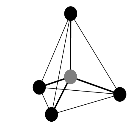
Figure 10: Geometry of stringlike pentaquarks

The vibrational spectrum of the stringlike $q^{4}\bar{q}$ configuration with tetrahedral symmetry is characterized by four normal modes

$$M^{2}_{\rm vib}\;=\;\kappa_{1}\,v_{1}+\kappa_{2}\,\left(v_{2a}+v_{2b}\right)+\kappa_{3}\,\left(v_{3a}+v_{3b}+v_{3c}\right)+\kappa_{4}\,\left(v_{4a}+v_{4b}+v_{4c}\right)~{},$$ (56)

where $v_{1}$ refers to the symmetric stretching vibration (breathing mode), and $v_{2a}+v_{2b}=v_{2}$ and $v_{4a}+v_{4b}+v_{4c}=v_{4}$ to bending modes of the four-quark configuration, whereas $v_{3a}+v_{3b}+v_{3c}=v_{3}$ correspond to the relative vibration of the antiquark with respect to the four-quark system [43]. The radial excitations of the stringlike configuration of Fig. 10 consists of a series of vibrational excitations labeled by $(v_{1},v_{2},v_{3},v_{4})$ and a tower of rotational excitations built on top of each vibration. For the simple case that is being considered here (model space with $N=1$), the wave functions in the stringlike model coincide with those of the harmonic oscillator quark model.

4.3 Wave functions

The pentaquark wave function is obtained by combining the spin-flavor part with the color and orbital parts in such a way that the total wave function is a color-singlet, and that the four quarks satisfy the Pauli principle, i.e. are antisymmetric under any permutation of the four quarks. Since the color part of the pentaquark wave function is a $[222]$ singlet and that of the antiquark a $[11]$ anti-triplet, the color wave function of the four-quark configuration is a $[211]$ triplet which has $F_{1}$ symmetry under ${\cal T}_{d}$. The total $q^{4}$ wave function is antisymmetric ($A_{2}$), hence the orbital-spin-flavor part has to have $F_{2}$ symmetry

$$\psi_{A_{2}}\;=\;\left[\psi^{\rm c}_{F_{1}}\times\psi^{\rm osf}_{F_{2}}\right]_{A_{2}}~{}.$$ (57)

Here the square brackets $[\cdots]$ denote the tensor coupling under the tetrahedral group ${\cal T}_{d}$. In Table 9, I present the allowed spin-flavor multiplets with exotic pentaquarks for some lowlying orbital excitations. The exotic spin-flavor states associated with the state $L^{P}_{t}=0^{+}_{A_{1}}$ all belong to the $[42111]$ spin-flavor multiplet with $F_{2}$ symmetry. The corresponding orbital-spin-flavor wave function is given by

$$\psi^{\rm osf}_{F_{2}}\;=\;\left[\psi^{\rm o}_{A_{1}}\times\psi^{\rm sf}_{F_{2}}\right]_{F_{2}}~{}.$$ (58)

A radial excitation with $L^{P}_{t}=1^{-}_{F_{2}}$ gives rise to exotic pentaquark states of the $[51111]$, $[42111]$, $[33111]$ and $[32211]$ spin-flavor configurations with symmetry $A_{1}$, $F_{2}$, $E$ and $F_{1}$, respectively. They are characterized by the orbital-spin-flavor wave functions

$$\psi^{\rm osf}_{F_{2}}\;=\;\left[\psi^{\rm o}_{F_{2}}\times\psi^{\rm sf}_{t}\right]_{F_{2}}~{},$$ (59)

with $t=A_{1}$, $F_{2}$, $E$ and $F_{1}$.

Table 9: Discrete symmetry of exotic pentaquark states

$\psi$	$\psi^{\rm c}$	$\psi^{\rm osf}$	$\psi^{\rm o}$	$\psi^{\rm sf}$	Exotic spin-flavor
					configuration
$A_{2}$	$F_{1}$	$F_{2}$	$A_{1}$	$F_{2}$	$[42111]$
$A_{2}$	$F_{1}$	$F_{2}$	$F_{2}$	$A_{1}$	$[51111]$
			$F_{2}$	$F_{2}$	$[42111]$
			$F_{2}$	$E$	$[33111]$
			$F_{2}$	$F_{1}$	$[32211]$

4.4 Mass spectrum of $\Theta$ pentaquarks

The classification scheme of pentaquark states discussed in the previous sections is based only on the fact that quarks (and antiquarks) have orbital, color, spin and flavor degrees of freedom. These states form a complete basis. The precise ordering of the pentaquark states in the mass spectrum depends on the choice of a specific dynamical model (Skyrme, CQM, Goldstone boson exchange, instanton, hypercentral, stringlike, …). Since the available experimental information for pentaquark states is still being discussed and carefully (re)examined, I adopt a stringlike model in which the mass spectrum of $\Theta$ pentaquarks is described by the same mass formula as used for $q^{3}$ baryons in the previous section (see Eq. (38))

$$M^{2}\;=\;M_{0}^{2}+M_{\rm orb}^{2}+M_{\rm sf}^{2}~{}.$$ (60)

The orbital (or radial) excitations are given by

$$M_{\rm orb}^{2}\;=\;M_{\rm vib}^{2}+\alpha\,L~{},$$ (61)

where $M_{\rm vib}^{2}$ describes the vibrational spectrum of a tetrahedral $q^{4}\overline{q}$ configuration (see Eq. (56)). The rotational energies are given by a term linear in the orbital angular momentum $L$ which is responsable for the linear Regge trajectories in baryon and meson spectra. The spin-flavor part is expressed in the Gürsey-Radicati form of Eq. (39). The coefficients $\alpha$, $a$, $b$, $c$, $d$, $e$ and $f$ are taken from the previous study of baryon resonances, and the constant $M_{0}^{2}$ is determined by identifying the ground state exotic pentaquark with the recently observed $\Theta(1540)$ resonance. Since the lowest orbital states with $L^{P}_{t}=0^{+}_{A_{1}}$ and $1^{-}_{F_{2}}$ are interpreted as rotational states, for these excitations there is no contribution from the vibrational term $M^{2}_{\rm vib}$ to the mass of the corresponding pentaquark states. The state with $L^{P}_{t}=1^{-}_{A_{1}}$ belongs to a vibration between the four-quark system and the antiquark with $(v_{1},v_{2},v_{3},v_{4})=(0,0,1,0)$. The results for the lowest $\Theta$ pentaquarks (with strangeness ${\cal S}=+1$) are shown in Fig. 11.

Figure 11: Spectrum of $\Theta$ pentaquarks. Masses are given in MeV.

The lowest pentaquark belongs to the flavor antidecuplet (${}^{2S+1}\overline{10}$) with spin $S=1/2$ and isospin $I=0$. In the present calculation, the ground state pentaquark belongs to the $[42111]$ spin-flavor multiplet with $F_{2}$ symmetry, indicated in Fig. 11 by its dimension 1134, and an orbital excitation $0^{+}$ with $A_{1}$ symmetry. Therefore, the ground state has angular momentum and parity $J^{P}=1/2^{-}$. The first excited state at 1599 MeV is an isospin triplet $\Theta_{1}$-state of the 27-plet (${}^{2S+1}27$) with the same value of angular momentum and parity $J^{P}=1/2^{-}$. The lowest pentaquark state with positive parity occurs at 1668 MeV and belongs to the $[51111]$ spin-flavor multiplet (dimension 700) and an orbital excitation $1^{-}$ with $F_{2}$ symmetry. In the absence of a spin-orbit coupling, in this case there is a doublet with angular momentum and parity $J^{P}=1/2^{+}$, $3/2^{+}$.

4.5 Magnetic moments

Although it may be difficult to determine the value of the magnetic moment experimentally, it is an essential ingredient in calculations of the photo- and electroproduction cross sections [44, 45, 46]. Here I discuss the magnetic moment of negative parity antidecuplet states that are associated with the ground state $L^{P}_{t}=0^{+}_{A_{1}}$. They belong to the $[42111]$ spin-flavor multiplet with $F_{2}$ symmetry. The corresponding pentaquark wave function with angular momentum $J$ is given by Eqs. (57) and (58)

$$\psi^{(J)}_{A_{2}} = \left[\psi^{\rm c}_{F_{1}}\times\left[\psi^{\rm o}_{A_{1}}\times\psi^{\rm sf}_{F_{2}}\right]_{F_{2}}\right]^{(J)}_{A_{2}}$$ (62)

$$= \frac{1}{\sqrt{3}}\left[\psi^{\rm o}_{A_{1}}\left(\psi^{\rm c}_{F_{1\lambda}}\psi^{\rm sf}_{F_{2\rho}}-\psi^{\rm c}_{F_{1\rho}}\psi^{\rm sf}_{F_{2\lambda}}+\psi^{\rm c}_{F_{1\eta}}\psi^{\rm sf}_{F_{2\eta}}\right)\right]^{(J)}~{}.$$

The spin-flavor part can be expressed as a product of the antidecuplet flavor wave function $\phi_{E}$ and the $S=1/2$ spin wave function $\chi_{F_{2}}$

$$\psi^{\rm sf}_{F_{2\rho}}\;=\;\left[\phi_{E}\times\chi_{F_{2}}\right]_{F_{2}\rho} = -\frac{1}{2}\phi_{E_{\rho}}\chi_{F_{2\lambda}}-\frac{1}{2}\phi_{E_{\lambda}}\chi_{F_{2\rho}}+\frac{1}{\sqrt{2}}\phi_{E_{\rho}}\chi_{F_{2\eta}}~{},$$

$$\psi^{\rm sf}_{F_{2\lambda}}\;=\;\left[\phi_{E}\times\chi_{F_{2}}\right]_{F_{2}\lambda} = -\frac{1}{2}\phi_{E_{\rho}}\chi_{F_{2\rho}}+\frac{1}{2}\phi_{E_{\lambda}}\chi_{F_{2\lambda}}+\frac{1}{\sqrt{2}}\phi_{E_{\lambda}}\chi_{F_{2\eta}}~{},$$

$$\psi^{\rm sf}_{F_{2\eta}}\;=\;\left[\phi_{E}\times\chi_{F_{2}}\right]_{F_{2}\eta} = \frac{1}{\sqrt{2}}\phi_{E_{\rho}}\chi_{F_{2\rho}}+\frac{1}{\sqrt{2}}\phi_{E_{\lambda}}\chi_{F_{2\lambda}}~{}.$$ (63)

The coefficients in Eqs. (62) and (63) are a consequence of the tensor couplings under the tetrahedral group ${\cal T}_{d}$ (Clebsch-Gordon coefficients). The total angular momentum is $J=1/2$.

Since the orbital wave function has $L^{P}_{t}=0^{+}_{A_{1}}$, the magnetic moment only depends on the spin part. The magnetic moment of the $\Theta^{+}$ pentaquark can be obtained using the explicit form of the flavor $\phi$ and spin $\chi$ wave functions given in the appendices [47]

$$\mu_{\Theta^{+}}\;=\;\frac{1}{3}(2\mu_{u}+2\mu_{d}+\mu_{s})~{}.$$ (64)

In a similar way, the magnetic moments of the other exotic states of the antidecuplet, $\Xi_{3/2}^{+}$ and $\Xi_{3/2}^{--}$, are given by [47]

$$\mu_{\Xi_{3/2}^{--}}\;=\;\frac{1}{3}(\mu_{u}+2\mu_{d}+2\mu_{s})~{},\hskip 28.45274pt\mu_{\Xi_{3/2}^{+}}\;=\;\frac{1}{3}(2\mu_{u}+\mu_{d}+2\mu_{s})~{}.$$ (65)

These results are independent of the orbital wave functions, and are valid for any quark model in which the eigenstates have good $SU_{\rm sf}(6)$ spin-flavor symmetry. The values are in agreement with the results obtained in [48] for the MIT bag model [21].

In Table 10, I present the magnetic moments of the antidecuplet pentaquarks for angular momentum and parity $J^{P}=1/2^{-}$ together with their numerical values obtained using the same values of the quark magnetic moments as in the discussion of the $q^{3}$ baryons. The magnetic moments of the $J^{P}=1/2^{-}$ pentaquarks are typically an order of magnitude smaller than the proton magnetic moment. In Table 11 a comparison is presented with other theoretical predictions for negative parity pentaquarks.

Table 10: Magnetic moments of the ground state antidecuplet pentaquarks with $J^{P}=1/2^{-}$ in $\mu_{N}$

	$\mu_{\rm th}$	$\mu_{\rm calc}$
$\Theta^{+}$	$(6\mu_{u}+6\mu_{d}+3\mu_{s})/9$	$0.382$
$N^{0}$	$(5\mu_{u}+6\mu_{d}+4\mu_{s})/9$	$0.108$
$N^{+}$	$(6\mu_{u}+5\mu_{d}+4\mu_{s})/9$	$0.422$
$\Sigma^{-}$	$(4\mu_{u}+6\mu_{d}+5\mu_{s})/9$	$-0.166$
$\Sigma^{0}$	$(5\mu_{u}+5\mu_{d}+5\mu_{s})/9$	$0.148$
$\Sigma^{+}$	$(6\mu_{u}+4\mu_{d}+5\mu_{s})/9$	$0.462$
$\Xi^{--}_{3/2}$	$(3\mu_{u}+6\mu_{d}+6\mu_{s})/9$	$-0.440$
$\Xi^{-}_{3/2}$	$(4\mu_{u}+5\mu_{d}+6\mu_{s})/9$	$-0.126$
$\Xi^{0}_{3/2}$	$(5\mu_{u}+4\mu_{d}+6\mu_{s})/9$	$0.188$
$\Xi^{+}_{3/2}$	$(6\mu_{u}+3\mu_{d}+6\mu_{s})/9$	$0.502$

Table 11: Comparison of magnetic moments in $\mu_{N}$ of exotic antidecuplet pentaquarks with angular momentum and parity $J^{P}=1/2^{-}$

Method	Ref.	$\Theta^{+}$	$\Xi_{3/2}^{+}$	$\Xi_{3/2}^{--}$
Present	[47]	0.38	0.50	$-0.44$
MIT bag	[48]	0.37	0.45	$-0.42$
JW diquark	[44]	0.49
$KN$ bound state	[44]	0.31
Cluster	[45]	0.60
QCD sum rules	[49]	$0.12\pm 0.06^{\ast}$
	[50]	$0.24\pm 0.02^{\ast}$
	[51]	$0.18\pm 0.01^{\ast}$
Additive quarks	[52]	$0.43$		$-0.41$
∗ Absolute value

Finally, the magnetic moments of antidecuplet pentaquarks satisfy the generalized Coleman-Glashow sum rules [30, 31]

$$\mu_{\Theta^{+}}+\mu_{\Xi^{+}_{3/2}} = \mu_{N^{+}}+\mu_{\Sigma^{+}}~{},$$

$$\mu_{\Theta^{+}}+\mu_{\Xi^{--}_{3/2}} = \mu_{N^{0}}+\mu_{\Sigma^{-}}~{},$$

$$\mu_{\Xi^{--}_{3/2}}+\mu_{\Xi^{+}_{3/2}} = \mu_{\Xi^{-}_{3/2}}+\mu_{\Xi^{0}_{3/2}}~{},$$ (66)

and

$$2\mu_{\Sigma^{0}}\;=\;\mu_{\Sigma^{-}}+\mu_{\Sigma^{+}}\;=\;\mu_{N^{0}}+\mu_{\Xi^{0}_{3/2}}\;=\;\mu_{N^{+}}+\mu_{\Xi^{-}_{3/2}}~{}.$$ (67)

The same sum rules hold for the chiral quark-soliton model in the chiral limit [53].

In the limit of equal quark masses $m_{u}=m_{d}=m_{s}=m$, the magnetic moments of the antidecuplet pentaquark states (denoted by $i\in\overline{10}$) become proportional to the electric charges

$$\mu_{i}\;=\;\frac{1}{9}\frac{e}{2m}Q_{i}~{},$$ (68)

compared to $\mu_{i}=(e/2m)Q_{i}$ of Eq. (49) for the decuplet baryons. Just as for the baryon decuplet, in this limit the sum of the magnetic moments of all members of the antidecuplet vanishes identically $\sum_{i}\mu_{i}=0$.

5 Summary and conclusions

In these lecture notes, I reviewed some properties of baryons and pentaquarks in a stringlike collective model. The permutation symmetry among the quarks leads to definite geometric configurations: a nonlinear configuration for $q^{3}$ baryons in which the three constituent quarks are located at the corners of an equilateral triangle (oblate top), and a nonplanar configuration for $q^{4}\bar{q}$ pentaquarks in which the four quarks are located at the corners of an equilateral tetrahedron and the antiquark at its center. In this model, the radial excitations of the baryons and pentaquarks are interpreted as rotations and vibrations of the strings.

The algebraic structure of the model makes it possible to derive closed expressions for physical observables, such as masses and electromagnetic and strong couplings. An application to baryon resonances of the nucleon and delta families shows a good overall agreement with the available experimental data. An extension of the stringlike model to exotic baryons of the $\Theta$ family shows that the ground state pentaquark belongs to a flavor antidecuplet, has angular momentum and parity $J^{P}=1/2^{-}$ and, in comparison with the proton, has a small magnetic moment. The width is expected to be narrow due to a large suppression in the spatial overlap between the pentaquark and its decay products [42].

The first report of the discovery of the pentaquark has triggered an enormous amount of experimental and theoretical studies of the properties of exotic baryons. Nevertheless, there still exist many doubts and questions about the existence of this state since, in addition to various confirmations, there is an equal amount of experiments in which no signal has been observed. Hence, it is of the utmost importance to understand the origin between these apparently contradictory results, and to have irrefutable proof for or against the existence of pentaquarks. If confirmed, the measurement of the quantum numbers of the $\Theta(1540)$ and the excited pentaquark states, especially the angular momentum and parity, may help to distinguish between different models and to gain more insight into the relevant degrees of freedom and the underlying dynamics that determines the properties of exotic baryons. If not confirmed, remains the question whether pentaquarks exist or not, perhaps at a different mass. Theoretically, there is no reason why they should not exist. However, it is difficult to predict the mass in a model-independent way.

Appendix A Flavor wave functions

The states of a $SU(3)$ flavor multiplet are labeled by the isospin $I$, its projection $I_{3}$ and the hypercharge $Y$. All other flavor states can be obtained by applying ladder operators in flavor space and using the phase convention of De Swart [54]. Hence for each flavor multiplet it is sufficient to give the wave function of one member.

The flavor wave functions of the decuplet baryons (with $A_{1}$ symmetry) can be determined from the $\Delta^{++}$

$$\phi_{A_{1}}(\Delta^{++})\;=\;\left|uuu\right>~{},$$ (69)

and those of the octet baryons (with $E$ symmetry) from the proton wave function

$$\phi_{E_{\rho}}(p) = \left.\left.\frac{1}{\sqrt{2}}\right[\left|udu\right>-\left|duu\right>\right]~{},$$

$$\phi_{E_{\lambda}}(p) = \left.\left.\frac{1}{\sqrt{6}}\right[2\left|uud\right>-\left|udu\right>-\left|duu\right>\right]~{}.$$ (70)

Just as for the baryons, the flavor wave functions of the antidecuplet pentaquarks can be obtained by applying ladder operators in flavor space to the $\Theta^{+}$ wave function (with $E$ symmetry under ${\cal T}_{d}$)

$$\phi_{E_{\rho}}(\Theta^{+}) = -\left.\left.\frac{1}{2}\right[\left|duud\right>-\left|udud\right>+\left|uddu\right>-\left|dudu\right>\right]\bar{s}~{},$$

$$\phi_{E_{\lambda}}(\Theta^{+}) = -\left.\left.\frac{1}{2\sqrt{3}}\right[\left|duud\right>+\left|udud\right>-2\left|uudd\right>+\left|uddu\right>+\left|dudu\right>-2\left|dduu\right>\right]\bar{s}~{}.$$ (71)

Appendix B Spin wave functions

The spin of $q^{3}$ baryons can be either $S=3/2$ or $S=1/2$ (twice) with $A_{1}$ or $E$ symmetry under $D_{3}$, respectively. The corresponding wave functions are given by

$$\chi_{A_{1}}(q^{3})\;=\;\left|\uparrow\uparrow\uparrow\right>~{},$$ (72)

for $S=M_{S}=3/2$ and

$$\chi_{E_{\rho}}(q^{3}) = \left.\left.\frac{1}{\sqrt{2}}\right[\left|\uparrow\downarrow\uparrow\right>-\left|\downarrow\uparrow\uparrow\right>\right]~{},$$

$$\chi_{E_{\lambda}}(q^{3}) = \left.\left.\frac{1}{\sqrt{6}}\right[2\left|\uparrow\uparrow\downarrow\right>-\left|\uparrow\downarrow\uparrow\right>-\left|\downarrow\uparrow\uparrow\right>\right]~{},$$ (73)

for $S=M_{S}=1/2$. Note that the spin wave functions are related to the flavor wave functins of Eqs. (69) and (70) by interchanging $u$ by $\uparrow$ and $d$ by $\downarrow$. The spin states with $M_{S}\neq S$ are obtained by applying the lowering operator in spin space.

The spin of $q^{4}\bar{q}$ pentaquarks can be either $S=5/2$, $S=3/2$ (four times) or $S=1/2$ (five times) (see Table 8). The spin wave functions of antidecuplet pentaquarks of Eqs. (62) and (63) have $S=1/2$ and $F_{2}$ symmetry under the tetrahedral group. They arise as a combination of the spin wave function for the four-quark system with $S=1$ and $F_{2}$ symmetry and that of the antiquark with $S=1/2$

$$\chi_{F_{2\alpha}}(q^{4}\bar{q})\;=\;\sqrt{\frac{2}{3}}\;\chi_{F_{2\alpha}}(q^{4},M_{S}=1)\downarrow-\sqrt{\frac{1}{3}}\;\chi_{F_{2\alpha}}(q^{4},M_{S}=0)\uparrow~{},$$ (74)

with $\alpha=\rho$, $\lambda$, $\eta$. The $\uparrow$ and $\downarrow$ represent the spin of the antiquark. The spin wave functions of the four-quark system are given by

$$\chi_{F_{2\rho}}(q^{4},M_{S}=1) = \left.\left.-\frac{1}{\sqrt{2}}\,\right[\left|\downarrow\uparrow\uparrow\uparrow\right>-\left|\uparrow\downarrow\uparrow\uparrow\right>\right]~{},$$

$$\chi_{F_{2\lambda}}(q^{4},M_{S}=1) = \left.\left.-\frac{1}{\sqrt{6}}\,\right[\left|\downarrow\uparrow\uparrow\uparrow\right>+\left|\uparrow\downarrow\uparrow\uparrow\right>-2\left|\uparrow\uparrow\downarrow\uparrow\right>\right]~{},$$

$$\chi_{F_{2\eta}}(q^{4},M_{S}=1) = \left.\left.-\frac{1}{2\sqrt{3}}\,\right[\left|\downarrow\uparrow\uparrow\uparrow\right>+\left|\uparrow\downarrow\uparrow\uparrow\right>+\left|\uparrow\uparrow\downarrow\uparrow\right>-3\left|\uparrow\uparrow\uparrow\downarrow\right>\right]~{}.$$ (75)

The states with projection $M_{S}=0$ can be obtained by applying the lowering operator in spin space.

References

• [1] I. Estermann, R. Frisch and O. Stern, Nature 132, 169 (1933).
• [2] R. Hofstadter, Annu. Rev. Nucl. Sci. 7, 231 (1957).
• [3] J.I. Friedman and H.W. Kendall, Annu. Rev. Nucl. Sci. 22, 203 (1972).
• [4] M.K. Jones et al., Phys. Rev. Lett. 84, 1398 (2000);
O. Gayou et al., Phys. Rev. Lett. 88, 092301 (2002).
• [5] See e.g. C.E. Hyde-Wright and K. de Jager, Annu. Rev. Nucl. Part. Sci. 54, 217 (2004).
• [6] See e.g. V.D. Burkert and T.-S.H. Lee, Int. J. Mod. Phys. E 13, 1035 (2004) [arXiv:nucl-ex/0407020].
• [7] M. Gell-Mann and Y. Ne’eman, The Eightfold Way, (W.A. Benjamin, New York, 1964).
• [8] LEPS Collaboration, T. Nakano et al., Phys. Rev. Lett. 91, 012002 (2003).
• [9] See e.g. M. Karliner and H.J. Lipkin, Phys. Lett. B 597, 309 (2004) [arXiv:hep-ph/0405002];
Q. Zhao and F.E. Close, J. Phys. G: Nucl. Part. Phys. 31, L1 (2005) [arXiv:hep-ph/0404075];
K.H. Hicks, Progr. Part. Nucl. Phys., in press [arXiv:hep-ex/0504027];
A.R. Dzierba, C.A. Meyer and A.P. Szczepaniak, arXiv:hep-ex/0412077.
• [10] See e.g. B.K. Jennings and K. Maltman, Phys. Rev. D 69, 094020 (2004) [arXiv:hep-ph/0308286];
S.-L. Zhu, Int. J. Mod. Phys. A 19, 3439 (2004) [arXiv:hep-ph/0406204];
M. Oka, Progr. Theor. Phys. 112, 1 (2004) [arXiv:hep-ph/0406211];
R.L. Jaffe, Phys. Rep. 409, 1 (2005) [arXiv:hep-ph/0409065];
K. Goeke, H.-C. Kim, M. Praszałowicz and G.-S. Yang, Progr. Part. Nucl. Phys., in press [arXiv:hep-ph/0411195].
• [11] A.R. Dzierba, D. Krop, M. Swat, S. Teige and A.P. Szczepaniak, Phys. Rev. D 69, 051901 (2004) [arXiv:hep-ph/0311125];
K. Hicks, V. Burkert, A.E. Kudryavtsev, I.I. Strakovsky and S. Stepanyan, arXiv:hep-ph/0411265.
• [12] NA49 Collaboration, C. Alt et al., Phys. Rev. Lett. 92, 042003 (2004) [arXiv:hep-ex/0310014].
• [13] H1 Collaboration: A. Aktas et al., Phys. Lett. B 588, 17 (2004) [arXiv:hep-ex/0403017].
• [14] M. Hamermesh, Group theory and its application to physical problems, (Dover Publications, New York, 1989).
• [15] F.E. Close, An introduction to quarks and partons, (Academic Press, London, 1979)
• [16] Fl. Stancu, Group theory in subnuclear physics, (Oxford University Press, Oxford, 1996).
• [17] R.L. Jaffe, Phys. Rev. D 15, 267 (1977); ibid. 15, 281 (1977); ibid. 17, 1444 (1978).
• [18] A.Th.M. Aerts, P.J.G. Mulders and J.J. de Swart, Phys. Rev. D 17, 260 (1978); ibid. 21, 1370 (1980); ibid. 21, 2653 (1980).
• [19] R.L. Jaffe, in Proceedings of the Topical Conference on Baryon Resonances, Oxford, July 5-9, 1976, Eds. R.T. Ross and D.H. Saxon.
• [20] H. Högaasen and P. Sorba, Nucl. Phys. B 145, 119 (1978);
M. de Crombrugghe, H. Högaasen and P. Sorba, Nucl. Phys. B 156, 347 (1979);
C. Roiesnel, Phys. Rev. D 20, 1646 (1979).
• [21] D. Strottman, Phys. Rev. D 20, 748 (1979).
• [22] R. Bijker, F. Iachello and A. Leviatan, Ann. Phys. (N.Y.) 236, 69 (1994); ibid. 284, 89 (2000).
• [23] N. Isgur and G. Karl, Phys. Rev. D 18, 4187 (1978); ibid. 19, 2653 (1979); ibid. 20, 1191 (1979).
• [24] F. Iachello, N.C. Mukhopadhyay and L. Zhang, Phys. Lett. B 256, 295 (1991); Phys. Rev. D 44, 898 (1991).
• [25] K. Johnson and C.B. Thorn, Phys. Rev. D 13, 1934 (1974);
I. Bars and A.J. Hanson, Phys. Rev.D 13, 1744 (1974).
• [26] F. Gürsey and L.A. Radicati , Phys. Rev. Lett. 13, 173 (1964).
• [27] S. Capstick and N. Isgur, Phys. Rev. D 34, 2809 (1986).
• [28] Particle Data Group, Phys. Lett. B 592, 1 (2004).
• [29] M.A.B. Bég, B.W. Lee and A. Pais, Phys. Rev. Lett. 13, 514 (1964).
• [30] S. Coleman and S.L. Glashow, Phys. Rev. Lett. 6, 423 (1961).
• [31] S.-T. Hong and G.E. Brown, Nucl. Phys. A 580, 408 (1994).
• [32] H.-C. Kim, M. Praszałowicz and K. Goeke, Phys. Rev. D 57, 2859 (1998).
• [33] D. Diakonov, V. Petrov and M. Polyakov, Z. Phys. A 359, 305 (1997);
H. Weigel, Eur. Phys. J. A 2, 391 (1998);
M. Praszałowicz, Phys. Lett. B 575, 234 (2003) [arXiv:hep-ph/0308114];
J. Ellis, M. Karliner and M. Praszałowicz, JHEP 0405, 002 (2004) [arXiv:hep-ph/0401127].
• [34] S.L. Zhu, Phys. Rev. Lett. 91, 232002 (2003) [arXiv:hep-ph/0307345];
J. Sugiyama, T. Doi and M. Oka, Phys. Lett. B 581, 167 (2004) [arXiv:hep-ph/0309271].
• [35] T.D. Cohen and R.F. Lebed, Phys. Lett. B 578, 150 (2004) [arXiv:hep-ph/0309150];
T.D. Cohen, Phys. Lett. B 581, 175 (2004) [arXiv:hep-ph/0309111];
P.V. Pobylitsa, Phys. Rev. D 69, 074030 (2004) [arXiv:hep-ph/0310221];
E. Jenkins and A.V. Manohar, Phys. Rev. Lett. 93, 022001 (2004) [arXiv:/0401190]; JHEP 0406, 039 (2004) [arXiv:0402024];
D. Pirjol and C. Schat, Phys. Rev. D 71, 036004 (2005) [arXiv:hep-ph/0408293].
• [36] F. Csikor, Z. Fodor, S.D. Katz and T.G. Kovács, JHEP 0311, 070 (2003) [arXiv:hep-lat/0309090];
S. Sasaki, Phys. Rev. Lett. 93, 152001 (2004) [arXiv:hep-lat/0310014];
T.-W. Chiu and T.-H. Hsieh, arXiv:hep-ph/0403020;
N. Mathur et al., Phys. Rev. D 70, 074508 (2004) [arXiv:hep-ph/0406196];
N. Ishii, T. Doi, H. Iida, M. Oka, F. Okiharu and H. Suganuma, Phys. Rev. D 71, 034001 (2005) [arXiv:hep-lat/0408030];
B.G. Lasscock et al., arXiv:hep-lat/0503008;
F. Csikor, Z. Fodor, S.D. Katz, T.G. Kovács and B.C. Toth, arXiv:hep-lat/0503012;
C. Alexandrou and A. Tsapalis, arXiv:hep-lat/0503013;
T.T. Takahashi, T. Umeda, T. Onogi and T. Kunihiro, arXiv:hep-lat/0503019;
K. Holland and K.J. Juge, arXiv:hep-lat/0504007.
• [37] R. Jaffe and F. Wilczek, Phys. Rev. Lett. 91, 232003 (2003) [arXiv:hep-ph/0307341];
M. Karliner and H.J. Lipkin, Phys. Lett. B 575, 249 (2003) [arXiv:hep-ph/0402260];
E. Shuryak and I. Zahed, Phys. Lett. B 589, 21 (2004) [arXiv:hep-ph/0310270].
• [38] Fl. Stancu, Phys. Rev. D 58, 111501 (1998);
C. Helminen and D.O. Riska, Nucl. Phys. A 699, 624 (2002);
A. Hosaka, Phys. Lett. B 571, 55 (2003) [arXiv:hep-ph/0307232];
L.Ya. Glozman, Phys. Lett. B 575, 18 (2003) [arXiv:hep-ph/0308232];
Fl. Stancu and D.O. Riska, Phys. Lett. B 575, 242 (2003) [arXiv:hep-ph/0307010];
C.E. Carlson, Ch.D. Carone, H.J. Kwee and V. Nazaryan, Phys. Lett. B 573, 101 (2003) [arXiv:hep-ph/0307396]; ibid. 579, 52 (2004) [arXiv:hep-ph/0310038].
• [39] R. Bijker, M.M. Giannini and E. Santopinto, Eur. Phys. J. A 22, 319 (2004) [arXiv:hep-ph/0310281].
• [40] P. Kramer and M. Moshinsky, Nucl. Phys. 82, 241 (1966);
Fl. Stancu, Phys. Rev. D 58, 111501 (1998).
• [41] R. Bijker, M.M. Giannini and E. Santopinto, in Nuclear Physics, Large and Small, Eds. R. Bijker, R.F. Casten and A. Frank, AIP Conference Proceedings 726, 181 (2004) [arXiv:hep-ph/0405195]; Rev. Mex. Fís. 50 S2, 88 (2004) [arXiv:hep-ph/0312380]; arXiv:hep-ph/0409022.
• [42] X.-Ch. Song and S.-L. Zhu, Mod. Phys. Lett. A 19, 2791 (2004) [arXiv:hep-ph/0403093].
• [43] G. Herzberg, Molecular Spectra and Molecular Structure II. Infrared and Raman Spectra of Polyatomic Molecules, (Krieger Publishing Company, Malabar, Florida, 1991).
• [44] S.I. Nam, A. Hosaka and H.-Ch. Kim, Phys. Lett. B 579, 43 (2004).
• [45] Q. Zhao, Phys. Rev. D 69, 053009 (2004); Erratum ibid. 70, 039901 (2004) [arXiv:hep-ph/0310350];
Q. Zhao and J.S. Al-Khalili, Phys. Lett. B 582, 91 (2004). [arXiv:hep-ph/0312348].
• [46] K. Nakayama and K. Tsushima, Phys. Lett. B 583, 269 (2004) [arXiv:hep-ph/0311112].
• [47] R. Bijker, M.M. Giannini and E. Santopinto, Phys. Lett. B 595, 260 (2004) [arXiv:hep-ph/0403029].
• [48] Y.-R. Liu, P.-Z. Huang, W.-Z. Deng, X.-L. Chen and S.-L. Zhu, Phys. Rev. C 69, 035205 (2004) [arXiv:hep-ph/0312074].
• [49] P.-Z. Huang, W.-Z. Deng, X.-L. Chen and S.-L. Zhu, Phys. Rev. D 69, 074004 (2004) [arXiv:hep-ph/0311108].
• [50] Z.-G. Wang, W.-M. Yang and S.-L. Wan, arXiv:hep-ph/0501278.
• [51] Z.-G. Wang and R.-C. Hu, arXiv:hep-ph/0504273.
• [52] T. Inoue, V.E. Lyubovitskij, Th. Gutsche and A. Faessler, Progr. Theor. Phys. 113, 801 (2005) [arXiv:hep-ph/0408057].
• [53] H.-C. Kim and M. Praszałowicz, Phys. Lett. B 585, 99 (2004) [arXiv:hep-ph/0308242].
• [54] J.J. de Swart, Rev. Mod. Phys. 35, 916 (1963).