New exactly solvable reflectionless potentials of Gamov’s type

Abstract

In paper SUSY-hierarchies of one-dimensional potentials with continuous energy spectra are studied. Use of such hierarchies for analysis of reflectionless potentials is substantiated from the physical point of view. An interdependence (based on Darboux transformations) between spectral characteristics of potentials-partners is determined, an uniqueness of its solution in result of use of boundary conditions is shown. A rule of construction of new reflectionless potentials on the basis of known one is corrected, its proof is proposed. At first time a general solution for a superpotential $W_{n+m}(x)$ with an arbitrary number $n+m$ in the studied hierarchy on the basis of only one known partial solution for the superpotential $W_{n}(x)$ with the selected number $n$ is found.

A general solution of a hierarchy of inverse power (reflectionless) potentials is obtained. Such a hierarchy can be interesting as an example for solution of a known problem of search of general solutions of the hierarchies of different types (both in standard and parasupersymmetric quantum mechanics).

A consequent statement and analysis of exactly solvable reflectionless potentials of Gamov’s type, which at their shapes look qualitatively like scattering potentials in two-particle description of collisions between particles and nuclei or decay potentials in two-particle description of decay of compound spherical nuclear systems, are presented.

PACS numbers: 11.30.Pb 03.65.-w, 12.60.Jv 03.65.Xp, 03.65.Fd,

Keywords: supersymmetric quantum mechanics, exactly solvable model, reflectionless potentials, inverse power potentials, potentials of Gamov’s type, SUSY-hierarchy

1 Introduction

A widely known approach for analysis of properties of quantum systems and processes with their participation in nuclear physics of low and intermediate energies, in atomic and particle physics is based on study of characteristics of potentials, described these systems. Here, such an unusual phenomenon as resonant tunneling, which is shown in maximal values (close to one) of a penetrability coefficient of the potentials (and barriers concerned with them) at selected energy levels, has been caused a sufficient interest. This phenomenon allows to explain an existence of the resonant values of cross-sections of nuclear collisions, determines the resonant levels in the energy spectra for decays of the nuclei (where the decay probability is maximal), allows to predict half-value periods of the nuclear decays, leads to explanation of a number of other important effects. Because of this, methods of description of the resonant effects are developed intensively and are important.

A reflectionless penetration or an absolute transparence of the potentials (and the barriers concerned with them) of the quantum systems [5, 21], differed from the resonant tunneling by that it exists in the whole energy spectrum (or its large part), where a reflection coefficient is not only minimal but equals to zero, is more uncommon phenomenon. This effect is studied less sufficiently and looks more unusual from a point of view of common sense.

A lot of methods are developed for study of these and some other unusual quantum effects (for example, reinforcement of the barrier penetrability and breaking of tunneling symmetry in opposite directions during the penetration of multiple particles, absolute reflection at the above-barrier energies). Here, we note methods of direct and inverse problems of quantum mechanics, which are used the most widely. One note both monographs [6] and excellent reviews [21, 22], where both the methods for detailed study of the properties of the reflectionless one- and multichannel quantum systems (mainly, in the discrete energy spectra) and simple approaches for a qualitative analysis and a clear understanding of them are proposed.

Mainly, the methods of calculations of the spectral characteristics (wave functions, energy spectra) in the approaches pointed out above are approximated, while in extremely rare cases one can find types of the potentials, where exact analytical solutions exist. These potentials, named as exactly solvable potentials, have caused a large interest because of knowledge of the exact analytical form of the spectral characteristics gives a possibility to simplify maximally the problem of analysis of the properties of the quantum systems and, therefore, to understand them deeper. Therefore, a lot of papers are devoted to search of new types of the exactly solvable potentials. However, a number of such potentials, opened by the methods of the direct problems, are extremely small, and the found potentials are still far for an acceptable description of the real physical processes. The methods of the inverse problem sufficiently expand possibilities to resolve this problem (in a comparison on the methods of the direct approach), giving enough large variety of the own exactly solvable models, however for construction of the exact analytical forms of the potentials it needs often to know full sets of the wave functions and the levels in the energy spectra, and this account turned out an enough difficult process (and can be considered as an approximated calculating method with extremely high accuracy).

It turned out, that methods of supersymmetric quantum mechanics (SUSY QM), developed in last two and a half decades, are sufficiently more effective and enough simple in solution of these tasks, than the methods of direct and inverse problems. With their use one can obtain new exactly solvable potentials with their spectral characteristics. Here, I should like to note a fine review [8], to point out methods of Non-linear (Polynomial, $N$-fold …) supersymmetric quantum mechanics [1, 2]) developed intensively the last decade and given own original new solutions for the exactly solvable potentials, methods of the shape invariant potentials with different types of parameters transformations (for example, see [11, 9, 7, 10, 13, 14, 4, 3]), methods of description of the self-similar potentials studied by Shabat [18] and Spiridonov [19] in details and concerned with $q$-symmetry, methods of description of other types of the deformations of the potentials and symmetries (for example, see [12]). Also one can note a number of papers, connecting the methods of supersymmetry and the methods of inverse problem [21, 22] (with proposed literature list here).

As a separate subclass of the exactly solvable potentials, the methods of SUSY QM allow to choose a set of the reflectionless potentials. However, it failed to find the application of most of the found exactly solvable potentials for description of the real physical systems and processes.

It turned out, that in result of study of construction rules of SUSY-hierarchies of the potentials with taking into account of their energy spectra (both discrete and continuous ones) one can find the hierarchies which have own exactly solvable general solutions, and this gives new types of the reflectionless potentials which can be interesting from the physical point of view. In this paper we present a consequent receiving and analysis of the reflectionless potentials opened in [16], which in their consideration inside a spatial semi-axis have one hole and one barrier, after which they fall down to zero monotonously in the spatially asymptotic limit. Such potentials at their shape look like potentials of scattering in two-particle description of collisions between particles and nuclei or decay potentials in two-particle description of decay of compound spherical nuclear systems. Because of this, such potentials are named as the potentials of Gamov’s type. A large attention in paper is given to search of general solutions of the (reflectionless) SUSY-hierarchies of different types.

2 SUSY-interdependence between spectral characteristics of potentials-partners with continuous energy spectra

2.1 Darboux transformations

In the beginning let’s consider a formalism of Darboux transformations used widely in supersymmetric quantum mechanics (SUSY QM) [8] (see p. 275–276). Let’s consider a one-dimensional motion of a particle with mass $m$ inside a potential field $V(x)$. We introduce operators $A_{1}$ and $A_{1}^{+}$ of the following form:

$$\begin{array}[]{ll}A_{1}=\displaystyle\frac{\hbar}{\sqrt{2m}}\displaystyle\frac{d}{dx}+W_{1}(x),&A_{1}^{+}=-\displaystyle\frac{\hbar}{\sqrt{2m}}\displaystyle\frac{d}{dx}+W_{1}(x),\end{array}$$ (1)

where $W_{1}(x)$ is the function, defined on the whole spatial region with axis $x$. We assume that this function is continuous inside the whole region of its definition with the exception of some possible points of discontinuity.

On the basis of the operators $A_{1}$ and $A_{1}^{+}$ we construct Hamiltonians of the motion of the particle by two different ways (we find the Hamiltonians of Schrodinger type only):

$$\begin{array}[]{l}H_{1}=A_{1}^{+}A_{1}+C_{1}=-\displaystyle\frac{\hbar^{2}}{2m}\displaystyle\frac{d^{2}}{dx^{2}}+V_{1}(x),\\ H_{2}=A_{1}A_{1}^{+}+C_{1}=-\displaystyle\frac{\hbar^{2}}{2m}\displaystyle\frac{d^{2}}{dx^{2}}+V_{2}(x).\end{array}$$ (2)

In each case the Hamiltonian (2) is expressed through

own potential $V_{1}(x)$ or $V_{2}(x)$:

$$\begin{array}[]{ll}V_{1}(x)=W_{1}^{2}(x)-\displaystyle\frac{\hbar}{\sqrt{2m}}\displaystyle\frac{dW_{1}(x)}{dx}+C_{1},&V_{2}(x)=W_{1}^{2}(x)+\displaystyle\frac{\hbar}{\sqrt{2m}}\displaystyle\frac{dW_{1}(x)}{dx}+C_{1}.\end{array}$$ (3)

We see that two potentials are expressed through one common function $W_{1}(x)$. One can write:

$$V_{2}(x)=V_{1}(x)+2\displaystyle\frac{\hbar}{\sqrt{2m}}\displaystyle\frac{dW_{1}(x)}{dx}.$$ (4)

Construction of the potentials $V_{1}$ and $V_{2}$ of two quantum systems on the basis of one common function $W_{1}(x)$ establishes interdependence between the spectral characteristics (wave functions, energy spectra) of these systems. We shall consider this interdependence as the interdependence, defined by Darboux transformations. In development of SUSY QM theory the function $W_{1}(x)$ is named as superpotential, while the potentials $V_{1}(x)$ and $V_{2}(x)$ are named as supersymmetric potentials-partners (for example, see p. 275–276 in [8]).

Note, that one constant $C_{1}$ is introduced in the definitions (2) of the Hamiltonians of two quantum systems. If to use $C_{1}=E^{(1)}_{0}$ (here, $E^{(1)}_{0}$ is the lowest level of the energy spectrum of the first Hamiltonian $H_{1}$), then we obtain the most widely used construction of two Hamiltonians $H_{1}$ and $H_{2}$ on the basis of the operators $A_{1}$ and $A_{1}^{+}$ (for example, see p. 287–289 in [8]). If to use $C_{1}=0$, then we obtain the construction of the Hamiltonians of these two systems on the basis of the operators $A_{1}$ and $A_{1}^{+}$ as in [16] (see p. 443, sec. 2). At $E^{(1)}_{0}=0$ both approaches of construction of two Hamiltonians $H_{1}$ and $H_{2}$ are coincided:

$$\begin{array}[]{l}H_{1}=A_{1}^{+}A_{1}=-\displaystyle\frac{\hbar^{2}}{2m}\displaystyle\frac{d^{2}}{dx^{2}}+V_{1}(x),\\ H_{2}=A_{1}A_{1}^{+}=-\displaystyle\frac{\hbar^{2}}{2m}\displaystyle\frac{d^{2}}{dx^{2}}+V_{2}(x).\end{array}$$ (5)

2.2 Varieties of the SUSY-hierarchies

Let’s assume that there are new operators $A_{2}$ and $A_{2}^{+}$, on the basis of which the Hamiltonian $H_{2}$ of the second system can be written in the form:

$$H_{2}=A_{2}^{+}A_{2}+C_{2}=-\displaystyle\frac{\hbar^{2}}{2m}\displaystyle\frac{d^{2}}{dx^{2}}+V_{2}(x),$$ (6)

where a new constant $C_{2}$ is introduced. Then on the basis of Darboux transformations one can define SUSY-partner to the Hamiltonian $H_{2}$ — the Hamiltonian $H_{3}$ of the third system:

$$H_{3}=A_{2}A_{2}^{+}+C_{2}=-\displaystyle\frac{\hbar^{2}}{2m}\displaystyle\frac{d^{2}}{dx^{2}}+V_{3}(x).$$ (7)

By such a way one can define consecutively a new Hamiltonian $H_{n+1}$ (and a new potential $V_{n+1}$ concerned with it) with a next number $n+1$ on the basis of the known Hamiltonian $H_{n}$ (and the potential $V_{n}$) with the previous number $n$. Here, the following expressions are fulfilled:

$$\begin{array}[]{l}H_{n}=A_{n}^{+}A_{n}+C_{n}=-\displaystyle\frac{\hbar^{2}}{2m}\displaystyle\frac{d^{2}}{dx^{2}}+V_{n}(x),\\ H_{n+1}=A_{n}A_{n}^{+}+C_{n}=-\displaystyle\frac{\hbar^{2}}{2m}\par\displaystyle\frac{d^{2}}{dx^{2}}+V_{n+1}(x).\end{array}$$ (8)

A sequence of such Hamiltonians (and a sequence the potentials of these Hamiltonians) forms one SUSY-hierarchy. If to use $C_{n}=E_{0}^{(n)}$, then we obtain the most widely used (standard) definition of SUSY-hierarchy (for example, see p. 287–289 in [8]; here, methods of calculation of the energy spectra and wave functions for each potential of one hierarchy, the superpotentials concerned with them, are presented). But on this case the lowest level of the energy spectrum of each Hamiltonian with the next number in the hierarchy is located higher then the lowest levels of all Hamiltonians with the previous numbers. Usually, these hierarchies have the potentials, lower parts of the energy spectra of which are discrete.

It turned out, that if to change values of the constants $C_{n}$, than we obtain new types of SUSY-hierarchies with own exactly solvable potentials, which can be differed from the potentials of the hierarchy, defined by the way pointed out above. Here, if to use $C_{n}=0$, then we obtain the hierarchy of the potentials, studied in [16]. In such hierarchy the lowest level of the Hamiltonian with arbitrary number coincides with the lowest levels of the Hamiltonians with the other numbers. In particular, if to select $C_{n}=E_{0}^{(n)}=0$, then these hierarchies turn out to be convenient enough for connection together of the Hamiltonians with the continuous energy spectra completely, and their potentials turn out to be useful for study of real processes of particles and nuclei scattering (because of the scattering potentials tend to zero in asymptotic spatial regions). Therefore, the hierarchies of such a type are more useful from the physical point of view in study of collisions between particles and nuclei in a comparison on the most widely used type of the hierarchy presented, for example, in [8] (see p. 287-289), and their use is substantiated physically for study of the reflectionless potentials.

Because of this, we shall consider further just this case.

2.3 Interdependence between wave functions of the potentials-partners

Let’s consider two quantum systems with the continuous energy spectra. Then Darboux transformations allow to establish an interdependence between the wave functions of these systems. In accordance with (5), we write:

$$\begin{array}[]{l}H_{1}\varphi^{(1)}_{k}=A_{1}^{+}A_{1}\varphi^{(1)}_{k}=E^{(1)}_{k}\varphi^{(1)}_{k},\\ H_{2}\varphi^{(2)}_{k^{\prime}}=A_{1}A_{1}^{+}\varphi^{(2)}_{k^{\prime}}=E^{(2)}_{k^{\prime}}\varphi^{(2)}_{k^{\prime}},\end{array}$$ (9)

where $E^{(1)}_{k}$ and $E^{(2)}_{k^{\prime}}$ are the energy levels of these systems, $\varphi^{(1)}_{k}(x)$ and $\varphi^{(2)}_{k^{\prime}}(x)$ are the wave functions (eigen-functions) corresponding to these levels, $k=\displaystyle\frac{1}{\hbar}\sqrt{2mE^{(1)}_{k}}$ and $k^{\prime}=\displaystyle\frac{1}{\hbar}\sqrt{2mE^{(2)}_{k^{\prime}}}$ are wave vectors corresponding to the levels $E^{(1)}_{k}$ and $E^{(2)}_{k^{\prime}}$. From (9) we obtain:

$$H_{2}(A_{1}\varphi^{(1)}_{k})=A_{1}A_{1}^{+}(A_{1}\varphi^{(1)}_{k})=A_{1}(A_{1}^{+}A_{1}\varphi^{(1)}_{k})=A_{1}(E^{(1)}_{k}\varphi^{(1)}_{k})=E^{(1)}_{k}(A_{1}\varphi^{(1)}_{k}).$$ (10)

We see, that the function $f(x)=A_{1}\varphi^{(1)}_{k}(x)$ is the eigen-function of the operator $\hat{H}_{2}$ to a constant factor, i. e. it represents the wave function $\varphi^{(2)}_{k^{\prime}}(x)$ of the Hamiltonian $H_{2}$. The energy level $E^{(1)}_{k}$ must be the eigen-value of this operator exactly, i. e. it represents the energy level $E^{(2)}_{k^{\prime}}$ of this Hamiltonian. Here, new wave function and energy level have the same index ${k^{\prime}}$. One can write:

$$\begin{array}[]{lcr}A_{1}\varphi^{(1)}_{k}(x)=N_{2}\varphi^{(2)}_{k^{\prime}}(x),&E^{(1)}_{k}=E^{(2)}_{k^{\prime}},&N_{2}=const.\end{array}$$ (11)

Taking into account (9), we write:

$$H_{1}(A_{1}^{+}\varphi^{(2)}_{k^{\prime}})=A_{1}^{+}A_{1}(A_{1}^{+}\varphi^{(2)}_{k^{\prime}})=A_{1}^{+}(A_{1}A_{1}^{+}\varphi^{(2)}_{k^{\prime}})=A_{1}^{+}(E^{(2)}_{k^{\prime}}\varphi^{(2)}_{k^{\prime}})=E^{(2)}_{k^{\prime}}(A_{1}^{+}\varphi^{(2)}_{k^{\prime}})$$ (12)

and obtain:

$$\begin{array}[]{lcr}A_{1}^{+}\varphi^{(2)}_{k^{\prime}}(x)=N_{1}\varphi^{(1)}_{k}(x),&E^{(2)}_{k^{\prime}}=E^{(1)}_{k},&N_{1}=const.\end{array}$$ (13)

Therefore, we find the following interdependences between the wave functions and the energy levels for two systems SUSY-partners in regions of the continuous energy spectra:

$$\begin{array}[]{lcr}\varphi^{(1)}_{k}(x)=\displaystyle\frac{1}{N_{1}}A_{1}^{+}\varphi^{(2)}_{k^{\prime}}(x),&\varphi^{(2)}_{k^{\prime}}(x)=\displaystyle\frac{1}{N_{2}}A_{1}\varphi^{(1)}_{k}(x),&E^{(1)}_{k}=E^{(2)}_{k^{\prime}}.\end{array}$$ (14)

Conclusion: Expressions (14) prove, that the hierarchy, defined at $C_{n}=0$, establishes the interdependence (on the basis of Darboux transformations with the operators $A_{1}$ and $A_{1}^{+}$ of the form (1)) between the wave functions and the levels of the continuous energy spectra of the Hamiltonians-partners.

Consequence 1: One can calculate coefficients $N_{1}$ and $N_{2}$ uniquely from normalization conditions of the wave functions (for the continuous energy spectrum, with taking into account of boundary conditions) for each system. A selection and use of the boundary conditions make the solution of the interdependence between the wave functions of the potentials-partners with the continuous energy spectra as uniqueness (the interdependence (14) between the wave functions is corrected in a comparison on Exp. (14) in [16]).

Consequence 2: In accordance with (14), the energy levels of the Hamiltonians-partners with the continuous energy spectra of the hierarchy, defined at $C_{n}=0$, coincide between each other (as for the Hamiltonians of the hierarchy with the discrete energy spectra with a possible exception of the lowest levels; the SUSY-interdependence between the energy levels is corrected in a comparison on Exp. (14) in [16]).

Consequence 3: Uniquely interdependence between the wave functions and the energy levels of the systems-partners of the hierarchy, defined at $C_{n}=0$, establishes an uniquely interdependence between other characteristics of these systems, calculation of which is based on the wave functions and the energy spectra.

2.4 Interdependence between coefficients of penetrability and reflection

We shall consider a case when the superpotential $W_{1}(x)$ and the potentials $V_{1}(x)$ and $V_{2}(x)$ of two studied systems are finite in the whole spatial region of their definition. At $x\to\pm\infty$ one can write:

$$W_{1}(x\to\pm\infty)=W_{\pm}$$ (15)

and

$$V_{1}(x\to\pm\infty)=V_{2}(x\to\pm\infty)=W^{2}_{\pm}.$$ (16)

On this case one can determine amplitudes of transmission and reflection for the wave functions of these systems, and Darboux transformations establish an unique dependence between them (for example, see [8], p. 278–279).

Let’s consider a plane wave $e^{ik_{-}x}$ which propagates in a positive direction of the axis $x$ inside fields of two potentials $V_{1}(x)$ and $V_{2}(x)$ (we assume that this plane wave has the same wave vector $k_{-}$ for the fields of two potentials). Then in spatial asymptotic regions we obtain the transmitted waves $T_{1}(k_{-},k_{+})e^{ik_{+}x}$ and $T_{2}(k_{-},k_{+})e^{ik_{+}x}$, and the reflected waves $R_{1}(k_{-})e^{-ik_{-}x}$ and $R_{2}(k_{-})e^{-ik_{-}x}$ also. For the wave function one can write:

$$\begin{array}[]{ll}\varphi^{(1)}(k,x\to-\infty)\to\bar{N}_{1}(e^{ik_{-}x}+R_{1}e^{-ik_{-}x}),&\varphi^{(1)}(k,x\to+\infty)\to\bar{N}_{1}T_{1}e^{ik_{+}x},\\ \varphi^{(2)}(k,x\to-\infty)\to\bar{N}_{2}(e^{ik_{-}x}+R_{2}e^{-ik_{-}x}),&\varphi^{(2)}(k,x\to+\infty)\to\bar{N}_{2}T_{2}e^{ik_{+}x},\end{array}$$ (17)

where $k$, $k_{-}$ and $k_{+}$ are defined by such a way:

$$\begin{array}[]{lcr}k=\displaystyle\frac{1}{\hbar}\sqrt{2mE},&k_{-}=\displaystyle\frac{1}{\hbar}\sqrt{2m(E-W^{2}_{-})},&k_{+}=\displaystyle\frac{1}{\hbar}\sqrt{2m(E-W^{2}_{+})},\end{array}$$ (18)

and coefficients $\bar{N}_{1}$ and $\bar{N}_{2}$ can be obtained from the normalization conditions with taking into account of the potentials forms and the boundary conditions.

Using the asymptotic expressions (17) for the wave functions, taking into account the interdependence (14) between them and the definitions (1) for the operators $A_{1}$ and $A_{1}^{+}$, we obtain:

$$\begin{array}[]{l}\bar{N}_{1}\biggl{(}e^{ik_{-}x}+R_{1}e^{-ik_{-}x}\biggr{)}=\displaystyle\frac{\bar{N}_{2}}{N_{1}}\biggl{[}\biggl{(}W_{-}-\displaystyle\frac{ik_{-}\hbar}{\sqrt{2m}}\biggr{)}e^{ik_{-}x}+\biggl{(}W_{-}+\displaystyle\frac{ik_{-}\hbar}{\sqrt{2m}}\biggr{)}R_{2}e^{-ik_{-}x}\biggr{]},\\ \bar{N}_{1}T_{1}e^{ik_{+}x}=\displaystyle\frac{\bar{N}_{2}}{N_{1}}T_{2}\biggl{(}W_{+}-\displaystyle\frac{ik_{+}\hbar}{\sqrt{2m}}\biggr{)}\par e^{ik_{+}x}.\end{array}$$ (19)

These expressions are found only for the asymptotic spatial regions for the systems-partners of the hierarchy, defined at $C_{n}=0$. They are fulfilled only in a case when items with the same exponents are equal between each other. We obtain:

$$\frac{\bar{N}_{2}}{N_{1}}=\displaystyle\frac{\bar{N}_{1}}{W_{-}-\displaystyle\frac{ik_{-}\hbar}{\sqrt{2m}}}$$ (20)

and

$$\begin{array}[]{lr}R_{1}(k_{-})=R_{2}(k_{-})\displaystyle\frac{W_{-}+\displaystyle\frac{ik_{-}\hbar}{\sqrt{2m}}}{W_{-}-\displaystyle\frac{ik_{-}\hbar}{\sqrt{2m}}},&T_{1}(k_{-},k_{+})=T_{2}(k_{-},k_{+})\displaystyle\frac{W_{+}-\displaystyle\frac{ik_{+}\hbar}{\sqrt{2m}}}{W_{-}-\displaystyle\frac{ik_{-}\hbar}{\sqrt{2m}}}.\end{array}$$ (21)

Expressions (21) establish the unique interdependence between the amplitudes of the transmission and the reflection for two quantum systems (it agrees with Consequence 3, pointed out in the previous section). One can define coefficients of penetrability and reflection of the potentials $V_{1}(x)$ and $V_{2}(x)$ as squares of modules of the amplitudes of the transmission and the reflection. We see that all these coefficients are not depended on the normalized coefficients $N_{1}$, $N_{2}$, $\bar{N}_{1}$, $\bar{N}_{2}$ and they are defined relatively one selected energy level, along which the propagation of the wave is studied.

We note, that the expressions of the interdependences between the amplitudes (and the coefficients) of the transmission and the reflection are known mainly for the systems with the energy spectra, containing low discrete levels. We repeat their receiving for hierarchies of potentials (i. e. a lot of potentials) with the continuous energy spectra completely.

3 Search of a hierarchy of reflectionless potentials

Let’s consider a quantum system with a potential, which has zero coefficient of reflection. Then a wave function of such system has an amplitude of the reflection, which equals to zero also. We shall name these quantum systems and their potentials as reflectionless or absolutely transparent. Then from (21) one can see that a potential SUSY-partner (and a system corresponding to it) for the reflectionless potential is reflectionless also. Using this simple idea and knowing a form of only one reflectionless potential, one can construct a number of new (early unknown) exactly solvable reflectionless potentials.

3.1 A recurrent method of construction of new reflectionless potentials

Now we formulate the following

Rule: two potentials $V_{1}(x)$ and $V_{2}(x)$ are reflectionless, if the following conditions are fulfilled:

• these potentials are potentials SUSY-partners;

• one potential is reflectionless;

• asymptotic expressions for the wave functions for both potentials have forms

  $$\begin{array}[]{l}\varphi^{(1,2)}(k,x\to-\infty)\to e^{ikx}+R_{1,2}e^{-ikx},\\ \varphi^{(1,2)}(k,x\to+\infty)\to T_{1,2}e^{ik^{\prime}x},\end{array}$$ (22)

This Rule was proposed in [16] (see p. 447, sec. 3) and we correct its formulation in this paper. Its proof consists in fulfillment of the condition (21) for the potentials-partners with continuous energy spectra and its application to the reflectionless potentials. Here, we consider only such a hierarchy, where interdependences between spectral characteristics of the potentials-partners are based on Darboux transformations. It does not take into account operator transformations of non-linear supersymmetry [1, 2], which we do not study in this paper. However, this idea is applied in that case also.

A constant potential does not give the reflection for a plane wave in its propagation inside this potential. Because of this, one can consider the constant potential as the refectionless one. Therefore, we conclude:

Consequence 1: If a potential belongs to SUSY-hierarchy, which has the constant potential, and its wave function in asymptotic regions can be presented in the form (22), then this potential is reflectionless.

In [16] (see p. 447–448, sec. 3) there is the following

Supposition 1: A potential is reflectionless only in such a case, if it belongs to SUSY-hierarchy, which has the constant potential, and its wave function in the asymptotic regions can be written as (22).

One can formulate this supposition by another way

Supposition 2: a reason of the reflectionless property of any potential consists in its SUSY-interdependence with the constant potential.

A proof of the Rule, formulated above, is a needed condition (proof of necessity) of fulfillment of the Suppositions 1 and 2. However, a proof of sufficiency of these suppositions must to take into account all possible types of SUSY-interdependences between the

operators $A$ and $A^{+}$ of algebra of supersymmetry (Darboux transformations, operator transformations of non-linear supersymmetry are partial cases of this algebra) and we do not know it else.

On the basis of the Consequence 1, formulated above, one can construct by recurrent way a hierarchy of the reflectionless potentials, if to use the constant potential as the first (started) potential.

Here, if to use the constant potential of a form:

$$V_{1}(x)=A^{2}=\mbox{const}$$ (23)

(we shall take into account cases $A^{2}\leq 0$ and $A^{2}\geq 0$ at $A^{2}\in\mathcal{R}$), then one can find for it a general form of a superpotential (see (33) and (37) in p. 449–450 in [16]), which connects this potential with all possible types of the potentials-partners. After obtaining the superpotential, one can find all possible solutions for the potentials-partners to the constant potential. In accordance with [16] (see (34) and (38) in p. 450), this approach gives only five partial solutions for the potential-partner ($\alpha=\hbar/\sqrt{2m}$):

$$\begin{array}[]{l}V_{2}(x)=\left\{\begin{array}[]{cl}A^{2},&W^{2}_{1}(x)=A^{2};\\ \displaystyle\frac{2\alpha^{2}}{(x+x_{0})^{2}},&W^{2}_{1}(x)\neq A=0\mbox{ and }x+x_{0}\neq 0;\\ |A|^{2}\left(1+\displaystyle\frac{2}{\sinh^{2}\bigl{(}|A|(x+x_{0})/\alpha\bigr{)}}\right),&A^{2}>0\mbox{ and }|W_{1}(x)|>|A|;\\ |A|^{2}\left(1-\displaystyle\frac{2}{\cosh^{2}\bigl{(}|A|(x+x_{0})/\alpha\bigr{)}}\right),&A^{2}>0\mbox{ and }|W_{1}(x)|<|A|;\\ |A|^{2}\left(\displaystyle\frac{2}{\cos^{2}\bigl{(}|A|(x+x_{0})/\alpha\bigr{)}}-1\right),&A^{2}<0\mbox{ and }W_{1}^{2}(x)\neq A^{2}\end{array}\right.\end{array}$$ (24)

and there are no other solutions. Further, with use of the Rule, formulated above, from the found five solutions of the system (24) one can select the reflectionless potentials, which form the general solution for the reflectionless potential-partner to the constant potential. Here, in accordance with the third point of the Rule, the fifth solution of the system (24) cannot be reflectionless potential, because of its wave function cannot be presented in the form (22). An effectiveness of introduction of the third point into the Rule (unlike the approach in [8] and other papers, known to us and concerned with the reflectionless potentials) is shown in this.

Further, using the found reflectionless potentials of the system (24), one can obtain on the basis of the Consequence 1 new reflectionless potentials with the next numbers and, therefore, construct sequentially by recurrent way the hierarchy of the reflectionless potentials.

3.2 A general solution for a superpotential with an arbitrary number

For finding the superpotential $W_{n}(x)$ with the selected number $n$ in the hierarchy, it needs to solve the Ricatti equation. In accordance with [20] (see p. 29), in a general case this equation cannot be integrated. However, it has one property: if we know one a partial solution of this equation, then one can reduce this equation to the Bernoulli equation and find its general solution.

As we found above, one can obtain the general solution for the superpotential $W_{1}(x)$, connected the constant potential with its potential-partner.

Now we assume, that we know a partial solution for a superpotential $\tilde{W}_{n}(x)$ with a number $n$ in the hierarchy. Then from the following transformations ($\alpha=\hbar/\sqrt{2m}$)

$$\begin{array}[]{l}\left.\begin{array}[]{l}V_{n+1}(x)=W_{n}^{2}(x)+\alpha\displaystyle\frac{dW_{n}(x)}{dx};\\ V_{n+1}(x)=W_{n+1}^{2}(x)-\alpha\displaystyle\frac{dW_{n+1}(x)}{dx}\end{array}\right\}\par\Longrightarrow\end{array}$$

$$\begin{array}[]{ll}\Longrightarrow&W_{n+1}^{2}(x)-\alpha\displaystyle\frac{dW_{n+1}(x)}{dx}=W_{n}^{2}(x)+\alpha\displaystyle\frac{dW_{n}(x)}{dx}.\end{array}$$ (25)

one can see, that a partial solution (early unknown) for a superpotential $\tilde{W}_{n+1}(x)$ with a next number $n+1$ in the hierarchy can be presented in the form:

$$\tilde{W}_{n+1}(x)=-\tilde{W}_{n}(x).$$ (26)

Therefore, we have proved, that in one SUSY-hierarchy, which is defined at $C_{n}=0$, there are two partial solutions for the superpotentials with the neighboring numbers, which are connected by (26).

Further, knowing the parial solution for the superpotential $\tilde{W}_{n+1}(x)$ with the number $n+1$, by such a way one can find a partial solution for a superpotential $\tilde{W}_{n+2}(x)$ with a next number $n+2$, which coincides with the superpotential $\tilde{W}_{n}(x)$. Continuing this logics further, we obtain recurrently an expression for a partial solution for a superpotential $\tilde{W}_{n+m}(x)$ with an arbitrary number $n+m$:

$$\tilde{W}_{n+m}(x)=(-1)^{m}\tilde{W}_{n}(x).$$ (27)

Here, we have proved, that in one SUSY-hierarchy, defined at $C_{n}=0$, for the known partial solution for the superpotential $\tilde{W}_{n}(x)$ with the selected number $n$ there is the partial solution for the superpotential $\tilde{W}_{n+m}(x)$ with the arbitrary number $n+m$, and these superpotentials are connected by (26) (it is found for the first time).

Conclusion:

• Knowing the partial solution for the superpotential $\tilde{W}_{n}(x)$ with the selected number $n$ in the hierarchy, one can find the partial solution for the superpotential $\tilde{W}_{n+1}(x)$ with the next number $n+1$ in the hierarchy by use of (26).

• Knowing the partial solution for the superpotential $\tilde{W}_{n}(x)$ with the selected number $n$ in the hierarchy, one can find the partial solution for the superpotential $\tilde{W}_{n+m}(x)$ with the arbitrary number $n+m$ in the hierarchy by use of (27) (it is found for the first time).

Further, knowing the partial solution for the superpotential $\tilde{W}_{n+m}(x)$, we shall find its general solution. Let’s solve the Ricatti equation (25), rewriting it in the form:

$$\frac{dW_{n+m}(x)}{dx}-\displaystyle\frac{1}{\alpha}W_{n+m}^{2}(x)=-\displaystyle\frac{F(x)}{\alpha}.$$ (28)

A change

$$y(x)=\displaystyle\frac{1}{W_{n+m}(x)-\tilde{W}_{n+m}(x)}$$ (29)

transforms the equation (28) into the form:

$$\frac{dy(x)}{dx}+\displaystyle\frac{2\tilde{W}_{n+m}(x)}{\alpha}y(x)=-\displaystyle\frac{1}{\alpha}.$$ (30)

A general solution of this equation is:

$$y(x)=e^{-\displaystyle\int\displaystyle\frac{2\tilde{W}_{n+m}(x)}{\alpha}dx}\Biggl{(}C_{1}-\displaystyle\frac{1}{\alpha}\displaystyle\int e^{\displaystyle\int\displaystyle\frac{2\tilde{W}_{n+m}(x)}{\alpha}dx}dx\Biggl{)}.$$ (31)

where $C_{1}$ is a constant of integration. We write this equation in the old variables:

$$W_{n+m}(x)=\displaystyle\frac{1}{y(x)}+\tilde{W}_{n+m}(x)=\displaystyle\frac{\mathstrut\alpha e^{\textstyle\frac{2}{\alpha}\displaystyle\int\tilde{W}_{n+m}(x)dx}}{\alpha C_{1}-\displaystyle\int e^{\textstyle\frac{2}{\alpha}\displaystyle\int\tilde{W}_{n+m}(x)dx}dx}+\tilde{W}_{n+m}(x).$$ (32)

Rewrite this solution through the given superpotential $\tilde{W}_{n}(x)$ with the selected number $n$:

$$W_{n+m}(x)=\displaystyle\frac{\mathstrut\alpha e^{(-1)^{m}\textstyle\frac{2}{\alpha}\displaystyle\int\tilde{W}_{n}(x)dx}}{\alpha C_{1}-\displaystyle\int e^{(-1)^{m}\textstyle\frac{2}{\alpha}\displaystyle\int\tilde{W}_{n}(x)dx}dx}+(-1)^{m}\tilde{W}_{n}(x).$$ (33)

Therefore, we have found the general solution for the superpotential $W_{n+m}(x)$ with the arbitrary number $n+m$ in the hierarchy on the basis of the known partial solution for the superpotential $\tilde{W}_{n}(x)$ with the selected number $n$ (it is found for the first time). Obtaining the general solution for the superpotential with the selected number, one can calculate further (uniquely) a general solution for the potentials-partners, connected with this superpotential. So, one can determine a general solution for SUSY-hierarchy, which is defined at $C_{n}=0$ and when only one partial solution for the superpotential with the selected number is known for it.

If to use the constant potential as the first potential, then the method described above allows to construct a general form of the hierarchy of the reflectionless potentials, defined at $C_{n}=0$. We note, that in [16] a recurrent approach for construction of the general solution for the hierarchy of the reflectionless potentials was proposed only.

The formula for the superpotential has the integral form and contains a dependence on one arbitrary constant of integration $C_{1}$. Changing this constant, one can change the shape of the potentials-partners, connected with this superpotential, without replacement of locations of the energy levels. Therefore, we have obtained a set of isospectral potentials with the same numbers in the hierarchy.

4 Construction of new exactly solvable reflectionless potentials

4.1 Hierarchy of inverse power potentials: a general solution

Let’s consider the second solution of the system (24). As it is shown in [16] (see p. 452–454, sec. 5.1.1) and in [15], this potential can be reflectionless and it has been causing an interest for study of properties of the reflectionless potentials.

We shall construct a hierarchy, which includes the potentials of such inverse power type only. In a general case one can write the potential $V_{n}(x)$ of this hierarchy in a form:

$$V_{n}(x)=\left\{\begin{array}[]{ll}\gamma_{n}\displaystyle\frac{\alpha^{2}}{(x-x_{0})^{2}},&\mbox{at }x<0;\\ \gamma_{n}\displaystyle\frac{\alpha^{2}}{(x+x_{0})^{2}},&\mbox{at }x>0,\end{array}\right.$$ (34)

where $\gamma_{n}=const$.

At first, we shall find a superpotential $W_{n}(x)$, concerned with this potential, supposing that this potential is known. One can determine the superpotential from the following equation:

$$\alpha\displaystyle\frac{dW_{n}(x)}{dx}=W_{n}^{2}(x)-V_{n}(x).$$ (35)

In [16] a partial solution $\tilde{W}_{n}(x)$ of this equation, which determines a potential-partner $V_{n+1}(x)$ of the inverse power type (34) with a next number $n+1$ in the hierarchy, was found (we write it for $x>0$):

$$\begin{array}[]{ll}\tilde{W}_{n}(x)=-\displaystyle\frac{\beta_{n}}{x+x_{0}},&\beta_{n}=const.\end{array}$$ (36)

As we see, this solution has the inverse power form (and it can be tested by a simple substitution into the equation (35) with taking into account (34)). Let’s find a general solution of the superpotential $W_{n}(x)$, defined by the equation (35). We see, that this equation (35) looks like the equation (27) (where it needs to replace the indexes $n+1\to n$ and the functions $F(x)\to V_{n}(x)$). Therefore, the general solution for the superpotential $W_{n}(x)$ can be written in the form (32), where one need to use the solution (36) as the partial solution. We obtain:

$$W_{n}(x)=\left\{\begin{array}[]{cl}\displaystyle\frac{2\beta_{n}-\alpha}{C_{1}(2\beta_{n}-\alpha)\bar{x}^{2\beta_{n}/\alpha}+\bar{x}}-\displaystyle\frac{\beta_{n}}{\bar{x}},&\mbox{at }2\beta_{n}\neq\alpha;\\ \displaystyle\frac{\alpha}{\bar{x}}\biggl{(}\displaystyle\frac{1}{\alpha C_{1}-\log{\bar{x}}}-\displaystyle\frac{1}{2}\biggr{)},&\mbox{at }2\beta_{n}=\alpha,\end{array}\right.$$ (37)

where $\bar{x}=x-x_{0}$ at $x<0$ and $\bar{x}=x+x_{0}$ at $x>0$. The potential-partner $V_{n+1}(x)$ to the potential (34), defined by the superpotential (37), is not inverse power one in a general case and its shape is deformed at a change of the parameter $C_{1}$ (without replacement of locations of the energy levels in spectra).

If to require that the new potential-partner $V_{n+1}(x)$ must be the inverse power type (34) only, then we obtain uniquely a requirement (we consider a case $2\beta_{n}\neq\alpha$):

$$C_{1}=0,$$ (38)

which reduces the general solution (37) into the form (36). Therefore, we have proved the following

Property 1: the solution (36) for the superpotential $W_{n}(x)$ is its general solution, which defines the general form of the potentials of the inverse power type (38) in one hierarchy (it is found at the first time).

Substituting the solution (36) as the general solution into (35) and taking into account (34), we obtain $\beta_{n}$:

$$\begin{array}[]{ll}W_{n}(x)=\displaystyle\frac{-\alpha(1\pm\sqrt{4\gamma_{n}+1})}{2(x+x_{0})},&\beta_{n}=\displaystyle\frac{\alpha}{2}\biggl{(}1\pm\sqrt{4\gamma_{n}+1}\biggr{)}.\end{array}$$ (39)

From here we see, that there is the following

Property 2 (uniqueness of construction of the hierarchy of the inverse power potentials): the general solution of the superpotential $W_{n}(x)$, which determines uniquely the potential-partner $V_{n+1}(x)$ with the next number $n+1$ in the hierarchy, is determined uniquely by the given potential $V_{n}(x)$ with the previous number $n$ (i. e. its coefficients $\gamma_{n}$) (it is found for the first time).

From (39) we obtain:

$$\begin{array}[]{lcl}V_{n+1}(x)&=&W_{n}^{2}(x)+\alpha\displaystyle\frac{dW_{n}(x)}{dx}=\biggl{(}1+\gamma_{n}\pm\sqrt{4\gamma_{n}+1}\biggr{)}\displaystyle\frac{\alpha^{2}}{(x+x_{0})^{2}}.\end{array}$$ (40)

We have found the general form of the potential in the hierarchy of the inverse power potentials (unlike [16], see p. 452–455, sec. 5.1.2, where the partial solution was found only). We write it in such a form:

$$\begin{array}[]{ll}V_{n}(x)=\left\{\begin{array}[]{ll}\gamma_{n}\displaystyle\frac{\alpha^{2}}{(x-x_{0})^{2}},&\mbox{at }x<0;\\ \gamma_{n}\displaystyle\frac{\alpha^{2}}{(x+x_{0})^{2}},&\mbox{at }x>0;\\ \end{array}\right.&\gamma_{n\pm 1}=1+\gamma_{n}\pm\sqrt{4\gamma_{n}+1}.\end{array}$$ (41)

If to use the constant potential as the first (starting) potential $V_{1}(x)$ in this hierarchy (and, therefore, we use $\gamma_{1}=0$), then in accordance with the Consequence 1, formulated and proved in sec. 3.1, the hierarchy of the inverse power potentials (41) becomes the hierarchy of the reflectionless inverse power potentials and the solution (41) becomes the general solution of the potential with the arbitrary number $n$ in this hierarchy.

Using the recurrent expressions (41), one can calculate values of the coefficients $\gamma_{n}$ with next numbers in this hierarchy. We write first some values

$$\gamma_{n}=0,2,6,12,20,30,42...$$ (42)

Note, when the hierarchy of the inverse power potentials becomes

reflectionless, then the coefficients $\gamma$ become natural numbers.

So, we have shown, that knowing only one partial solution for the superpotential with the selected number in the hierarchy, defined at $C_{n}=0$, one can determine uniquely the general solution for all potentials in this hierarchy (with taking into account of needed form of these potentials), i. e. one can find the general solution for the hierarchy of the needed type. Such a hierarchy can be interesting as an example of solution of a known problem of a search of general solutions of hierarchies, defined at the different values of $C_{n}$. Here, in [8] (see p. 374, sec. 13.1) a problem of search of a general form of an interdependence between superpotentials with neighboring numbers in hierarchies of parasupersymmetric quantum mechanics, defined at $C_{n}=E_{n}^{(1)}$, is pointed out. In [17] non-linear equations, connected variables $W_{n}\pm W_{n-1}$ together, are obtained and are solved easily. However, it is not clear, how to obtain a form of the superpotential with a next number on the basis of the known superpotential with a previous number.

Note, that the hierarchy of the inverse power reflectionless potentials represents a solution, where the potential $V_{n}(x)$ with a selected number $n$ does not coincide with any other potential $V_{m}(x)$ with another number $m\neq n$ in this hierarchy. I. e. the solution for the general form of the superpotential of this hierarchy is not reduced to a simple change of a form:

$$W_{n+m}(x)=(-1)^{m}W_{n}(x).$$ (43)

4.2 Potentials of Gamov’s type

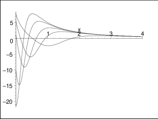
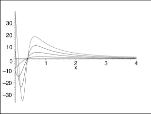
Fig. 1: A dependence of the potential $V_{n+1}(x)$ on $C_{1}$ and $\gamma$: (a) — the barrier maximum and the hole minimum of this potential are changed along the axis $x$ at the change of $C_{1}$ (at $C_{1}=0.01,0.1,0.3,1.0,2.5$, $\gamma=6$, $x_{0}=0.5$); (b) — the barrier maximum of this potential practically does not changed along the axis $x$ at the change of $\gamma$ (at $C_{1}=1$, $\gamma=2,6,12,20$, $x_{0}=0.5$).

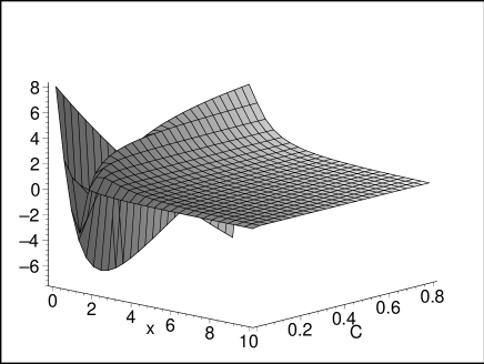
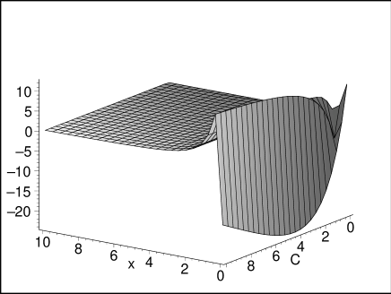
Fig. 2: New exactly solvable potential $V_{n+1}(x)$ of Gamov’s type (at $C_{n}\neq 0$). Continuous change of its shape at variation of $C_{1}$ ($\gamma=6$, $x_{0}=0.5$)

Let’s consider the superpotential (37) at $C_{1}\neq 0$ and at $2\beta_{n}\neq\alpha$. We shall find the potentials-partners, connected with it. We shall study them in the positive semi-axis $x\geq 0$ only. The potential $V_{n+1}(x)$ with the number $n+1$ is shown in Fig. 1 (a, b) for selected values of the parameters $C_{1}$ and $\gamma$. From these figures one can see, that this potential has one hole and one barrier, after which it falls down monotonously to zero with increasing of a spatial coordinate. In its behavior this potential looks qualitatively (at limit $x_{0}\to+0$) like potentials, used in theory of nuclear collisions for description of a scattering of particles on spherically symmetric nuclei, and also for description of decays and synthesis of nuclei with spherical shape. In Fig. 2 a continuous deformation of the shape of this potential at a change of the parameter $C_{1}$ is shown (here, one can analyze the deformation of the barrier and the hole of this potential). We see that at $C_{1}\to 0$ this potential tends to the inverse power potential. One can make sure in this also by a direct calculation of the superpotential (37), which tends to the form (36), and the potential tends to the form (41). At $C_{1}\neq 0$ the new potential is not inverse power one and, therefore, is the new exactly solvable solution. We note that one can consider it as an isospectral expansion of the early found potentials of the inverse power hierarchy (41).

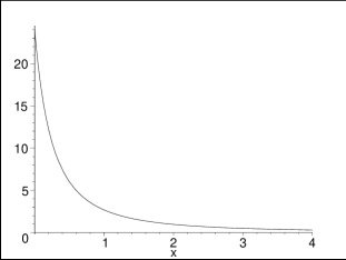
Fig. 3: Inverse-power potential $V_{n}(x)$ (at $C_{1}=1$, $\gamma=6$ and $x_{0}=0.5$). It does not depend on change of parameters $C_{1}$ and $\gamma$.

Another potential $V_{n}(x)$ SUSY-partner with a smaller number $n$ is shown in Fig. 3. We see that it has the inverse power dependence on the spatial coordinate. One can make sure that it is not deformed with the change of the coefficient $C_{1}$ and it belongs to the hierarchy of the inverse power potentials (41), studied in the previous section.

If to use the value of the parameter $\gamma$ from the succession (42), then the potential $V_{n}(x)$ becomes reflectionless, in accordance with the Rule, formulated above.

So, we have found the exactly solvable reflectionless potentials, which in their shape look qualitatively (at $x_{0}\to 0$ and $x_{0}\neq 0$), like the potentials of the scattering in description of the particles on nuclei of the spherical type, and also in description of the decays and synthesis of the nuclei of the spherical type.

If to study properties of the found potentials at the limit $x_{0}\to 0$, then one can conclude that these potentials are the potentials-partners to $\delta$-function, which has a peculiarity at zero. Because of this the found potentials must to have the peculiarity at zero also, and it is not clear, which penetration they have. However, a preliminary analysis has shown, that practically all part of such found potential without an enough small neighborhood at zero does not influence on the propagation of the particle in its field, because of it must be reflectionless. Then at a spherically symmetric consideration of the scattering of the particle in the field of this potential, a radial component of which represents the found potential, the particle propagates through it without the smallest reflection, and, therefore, without change of the angle of the propagation (except for an exact fall into a center). In this case one can conclude, that the found potential (in spite of it has the barrier) is reflectionless for the incident particle. If to use it for description of the scattering of the particle on a quantum system with the barrier, then one can conclude that such system must be unvisible for the incident particle, in spite of it has the scattering barrtier. Therefore, one can name the found potentials as the reflectionless potentials of Gamov’s type. At first time these potentials were opened in [16].

5 Conclusions

In the finishing, we note main conclusions and new results.

• We construct a hierarchy (defined at all coefficients $C_{n}=0$), where the lowest energy level of a Hamiltonian with an arbitrary number coincides with the lowest energy levels for Hamiltonians with other numbers. It has shown, that potentials of such hierarchies (defined at $C_{n}=E_{0}^{(n)}=0$) with continuous energy spectra correspond to real processes of scattering between particles and nuclei (because of the scattering potentials in the asymptotic spatial regions tend to zero) and, therefore, such hierarchies can be more useful from a physical point of view in study of the collisions between the particles and the nuclei in a comparison on the most widely used type of the hierarchy, where $C_{n}=E_{0}^{(n)}\neq 0$ (for example, see p. 287–289 in [8]).

  An application of such hierarchies in study of the reflectionless potentials has substantiated from the physical point of view.

• It has shown, that the hierarchy, defined at $C_{n}=0$, establishes an interdependence (on the basis of Darboux transformations) between wave functions and levels of the continuous energy spectra of the Hamiltonians-partners. For the first time it has shown, that an application of boundary conditions makes the interdependence between the wave functions and the energy levels of the Hamiltonians-partners with the continuous energy spectra unique, and a selection of the boundary conditions does not influence on the interdependence between amplitudes of transmission and reflection and between coefficients of penetrability and reflection.

• A Rule of determination of new reflectionless potentials on the basis of known ones has corrected (at first, it was formulated in [16], p. 447, sec. 3). A proof of its fulfillment has proposed.

• For the first time it has proved, that at a known partial solution for a superpotential $\tilde{W}_{n}(x)$ with a selected number $n$ in the SUSY-hierarchy, defined at $C_{n}=0$, there is a partial solution for a superpotential $\tilde{W}_{n+m}(x)$ with an arbitrary number $n+m$, and these superpotentials are connected by (26).

• For the first time a general solution for a superpotential $W_{n+m}(x)$ with an arbitrary number $n+m$ (and a general form of potentials-partners, connected with this superpotential) in a hierarchy, defined at $C_{n}=0$, has found at a supposition, that only one partial solution for the superpotential $\tilde{W}_{n}(x)$ with the selected number $n$ in this hierarchy is known.

• For the first time a general solution for a superpotential with an arbitrary number and a general form of potentials, connected with it, in the hierarchy, defined at $C_{n}=0$ and where the potentials have an inverse power dependence on a spatial coordinate (and where tunneling is possible), i. e. of the form $V(x)=\pm\alpha/|x-x_{0}|^{n}$ (where $\alpha$ and $x_{0}$ are constants, $n$ is a natural number), have obtained. A general solution for the hierarchy of the reflectionless inverse power potentials has found. These solutions are determined uniquely on the basis of the only one known solution for the superpotential with the selected number. The found hierarchies can be interesting as an example of solution of a known problem of search of the general form of the hierarchies, defined at different values $C_{n}$ (see p. 374, sec. 13.1 in [8]).

• A consequent statement and an analysis (with substantiation of some points, which are not taken into account in [16]) of the reflectionless potentials, which in the spatial semi-axis have one hole and one barrier, after which they fall down to zero monotonously, are presented (at first, these potentials are considered in [16]). Such potentials at their shape look qualitatively like scattering potentials in two-particle description of collisions between particles and nuclei or decay potentials in two-particle description of decay of compound spherical nuclear systems. One can name such potentials as the potentials of Gamov’s type.

We note that the found potentials of Gamov’s type can be interesting in that they are exactly solvable, at own shape they look qualitatively like the scattering potentials at description of the nuclear collisions, they have one barrier (and because of this, tunneling in them is possible) and they can be reflectionless.

References

- [1] Andrianov, A. A. and Sokolov, A. V., “Nonlinear supersymmetry in Quantum Mechanics: algebraic properties and differential representation”, Nuclear Physics B660, 25–50 (2003). arXiv:hep-th/0301062.
- [2] Andrianov, A. A. and Cannata, F., “Nonlinear supersymmetry for spectral design in quantum mechanics”, Journal of Physics A37, 10297–10323 (2004). arXiv:hep-th/0407077.
- [3] Balantekin, A. B., “Algebraic approach to shape invariance”, Physical Review A57, 4188–4191 (1998); quant-ph/9712018.
- [4] Barclay, D. T., Dutt, R., Gangopadhyaya, A., Khare, A., Pagnamenta, A. and Sukhatme, U., “New exactly solvable Hamiltonians: shape invariance and self-similarity”, Physical Review A48, 2786–2797 (1993); arxiv:hep-ph/9304313.
- [5] Chabanov, V. M. and Zakhariev, B. N., “Absolutely transparent multichannel systems. Unexpected peculiarities”, Physics Letters B 319 (1–3), 13–15 (1993).
- [6] Chadan, K. and Sabatier, P. C., Inverse problems in quantum scattering theory, Springer-verlag, New York (1977), 344 p.
- [7] Cooper, F., Ginocchio, J. N. and Khare, A., “Relationship between supersymmetry and solvable potentials”, Physical Review D 36 (8), 2458–2473 (1987).
- [8] Cooper, F., Khare, A. and Sukhatme, U., Supersymmetry and quantum mechanics, Physics Reports 251, 267–385 (1995); arXiv:hep-th/9405029.
- [9] Dutt, R., Khare, A. and Sukhatme, U. P., “Exactness of supersymmetric WKB spectra for shape invariant potentials”, Physics Letters B 181, 295 (1986).
- [10] Dutt, R., Khare, A. and Sukhatme, U., “Supersymmetry, shape invariance and exactly solvable potentials”, American Journal of Physics 56, 163–168 (1988).
- [11] Gendenshtein, L., “Derivation of exact spectra of the Schrodinger equation by means of supersymmetry”, JETP Lett. 38, 356–359 (1983).
- [12] Gómez-Ullate, D. , Kamran, N. and Milson, R., “The inverse Darboux transformation and exactly solvable deformations of shape-invariant potentials”, Journal of Physics A: Mathematical and General 37 (5–6), 1780–1804 (2004); [arXiv:quant-ph/0308062].
- [13] Khare, A. and Sukhatme, U. P., “Scattering amplitudes for supersymmetric shape invariant potentials by operator methods”, Journal of Physics A: Mathematical and General 21, L501–L508 (1988).
- [14] Khare, A. and Sukhatme, U. P., “New shape invariant potentials in supersymmetric quantum mechanics”, Journal of Physics A: Mathematical and General 26, L901–L904 (1993); arxiv:hep-th/9212147.
- [15] Maydanyuk, S. P., “One-dimensional inverse power reflectionless potentials ” (talk on the II Conference on High Energy Physics, Nuclear Physics and Accelerator Physics, March 1-5, 2004, Kharkov, Ukraine), Problems of atomic science and technology. Series: Nuclear Physics Investigations (44) 5, 22-25 (2004); arXiv:quant-ph/0404021.
- [16] Maydanyuk, S. P., “SUSY-hierarhy of one-dimensional reflectionless potentials”, Annals of Physics 316 (2), 440–465 (April, 2005); arXiv:hep-th/0407237.
- [17] Rubakov, V. and Spiridonov, V., “Parasupersymmetric quantum mechanics”, Modern Physics Letters A 3, 1337–1347 (1993).
- [18] Shabat, A., Inverse Problems 8, 303 (1992).
- [19] Spiridonov, V., “Exactly solvable potentials and quantum algebras”, Physical Review Letters 69 (3), 398–401 (1992); arXiv:hep-th/9112075.
- [20] Tihonov, A. N., Vasilieva, A. B. and Sveshnikov, A. G., Differentsialnie uravneniya, Nauka - Fizmatlit, Moskva (1998), 232 p. — [in Russian].
- [21] Zakhariev, B. N. and Chabanov, V. M., “Qualitative theory of control of spectra, scattering, decays (Quantum intuition lessons)”, Physics of elementary particles and atomic nuclei 25 (Iss. 6), 1561–1597 (1994) — [in Russian].
- [22] Zakhariev, B. N. and Chabanov, V. M., “On the qualitative theory of elementary transformations of one- and multicannel quantum systems in the inverse problem approach”, Physics of elementary particles and atomic nuclei 30 (Iss. 2), 277–320 (1999) — [in Russian].