Di-Electron Bremsstrahlung in Intermediate-Energy $pn$ and $Dp$ Collisions

Abstract

Invariant mass spectra of di-electrons stemming from bremsstrahlung processes are calculated in a covariant diagrammatical approach for the exclusive reaction $Dp\to p_{\rm sp}\,np\>e^{+}e^{-}$ with detection of a forward spectator proton, $p_{\rm sp}$. We employ an effective nucleon-meson theory for parameterizing the sub-reaction $np\to np\>e^{+}e^{-}$ and, within the Bethe-Salpeter formalism, derive a factorization of the cross section in the form ${d\sigma_{Dp\to p_{\rm sp}\,np\>e^{+}e^{-}}}/{dM}={d\sigma_{np\to\,np\>e^{+}e^{-}}}/{dM}\times$ kinematical factor related solely to the deuteron ($M$ is the $e^{+}e^{-}$ invariant mass). The effective nucleon-meson interactions, including the exchange mesons $\pi$, $\sigma$, $\omega$ and $\rho$ as well as excitation and radiative decay of $\Delta(1232)$, have been adjusted to the process $pp\to pp\>e^{+}e^{-}$ at energies below the vector meson production threshold. At higher energies, contributions from $\omega$ and $\rho$ meson excitations are analyzed in both, $NN$ and $Dp$ collisions. A relation to two-step models is discussed. Subthreshold di-electron production in $Dp$ collisions at low spectator momenta is investigated as well. Calculations have been performed for kinematical conditions envisaged for forthcoming experiments at HADES.

I Introduction

Di-electron production in scattering processes of hadrons at low energies can be described essentially as bremsstrahlung from incoming and outgoing charged particles. Several formulae for bremsstrahlung, obtained within different approximations, have been proposed (for a survey of theoretical approaches to bremsstrahlung reactions see e.g. tormoz ). With the focus on intermediate energies, a covariant approach based on an effective meson-nucleon theory to calculate the bremsstrahlung of di-electrons from nucleon-nucleon scattering has recently been presented in mosel_calc , continuing and extending the series of previous investigations Kapusta . In this model the effective parameters have been adjusted to describe elastic nucleon-nucleon ($NN$) and inelastic $NN\to NN\pi$ processes at intermediate energies; besides, the role of excitations of intermediate resonances has been studied within this approach and it is found that at intermediate energies the main contribution comes from $\Delta$ resonances (see also Ref. ernst ), whereas excitations of higher mass resonances can be neglected. The role of higher mass and spin nucleon resonances at energies near the vector meson ($\rho$, $\omega$ and $\phi$) production thresholds have been investigated in some detail for proton-proton collisions in several papers (see, e.g., Refs. nakayama ; fuchs and references therein quoted) with the conclusion that at threshold-near energies the inclusion of heavier resonances also leads to good description of data. However, as demonstrated in Refs. nakayama ; ourOmega calculations with a reasonable readjustment of the effective parameters can equally well describe the data without higher mass and spin resonances. In contrast, for di-electron production in photon and pion induced reactions excitations of low-lying as well as heavier resonances can play a role lutzNew .

In the present paper we extend the covariant model mosel_calc ; ourOmega , which is based on an effective meson nucleon theory with inclusion of $\Delta$ isobar contributions and vector meson dominance, to the exclusive process $Dp\to p_{\rm sp}\ np\ e^{+}e^{-}$ with incoming deuteron $D$ where the di-electron $e^{+}e^{-}$ is detected in coincidence with the fast spectator proton $p_{\rm sp}$. We calculate the cross section of di-electrons produced primarily in bremsstrahlung processes which, to some extent, can be considered as background contribution to other, more complicate processes. In order to preserve the covariance of the approach, the deuteron ground state and the corresponding matrix elements are treated within the Bethe-Salpeter (BS) formalism by making use of a realistic solution of the BS equation, obtained within the same effective meson nucleon theory solution .

Corresponding experiments are planned by the HADES collaboration at the heavy ion synchrotron SIS/GSI Darmstadt HADES . The outgoing neutron $n$ and proton $p$ may be reconstructed by the missing mass technique. The very motivation of such experiments is to pin down the bremsstrahlung component for $e^{+}e^{-}$ production in the tagged sub-reaction $np\to np\>e^{+}e^{-}$ holzman . Detailed knowledge of this reaction, together with the directly measurable reaction $pp\to pp\>e^{+}e^{-}$, is a necessary prerequisite for understanding di-electron emission in heavy-ion collisions. In heavy-ion collisions the di-electron rate is determined by the retarded photon self-energy in medium, which in turn is related to in-medium propagators of various vector mesons. In such a way the in-medium modifications of vector mesons become directly accessible.

A broader scope is to achieve a refined understanding of the nucleon-nucleon force at intermediate energies. Similar to meson production or real bremsstrahlung, the virtual bremsstrahlung processes probe some off-shell part of the amplitude providing more profound insights into the electromagnetic structure of hadrons, e.g., the electromagnetic form factors in the time-like region, not accessible in on-mass shell reactions. Another important issue of di-electron emission in $NN$ collisions is to supply additional information on vector meson production, in particular $\omega$ and $\phi$ mesons ourOmega ; ourphi , which is interesting in respect to the Okubo-Zweig-Iizuka rule ozi and hidden strangeness in the nucleon.

Our paper is organized as follows. In section II we consider di-electron production in elementary $NN$ collisions by parameterizing the amplitudes by corresponding Feynman diagrams. Parameters are adjusted to $pp$ collisions. In section III we extend the approach to deuteron-proton collisions by employing the Bethe-Salpeter formalism with a realistic solution obtained with one-boson-exchange kernel. Within the spectator mechanism picture we derive a factorization formula relating the reactions $Dp\to p_{\rm sp}pn\>e^{+}e^{-}$ and $np\to np\>e^{+}e^{-}$. The summary and discussion can be found in section IV. Compilations of useful formulae are summarized in Appendices A and B (where a link to two step models is outlined), while the Appendix C describes some details needed for deriving the factorization formula.

II Di-electrons from $NN$ collisions

II.1 Kinematics and Notation

We consider the exclusive $e^{+}e^{-}$ production in $NN$ reactions of the type

$$N_{1}(P_{1})+N_{2}(P_{2})\to N_{1}^{\prime}(P_{1}^{\prime})+N_{2}^{\prime}(P_{2}^{\prime})+e^{+}(k_{1})+e^{-}(k_{2})$$ (1)

(For an extension towards including hadronic inelasticities in semi-inclusive reactions cf. Haglin_Gale .) The invariant eight-fold cross section is

$$d^{8}\sigma=\frac{1}{2\sqrt{\lambda(s,m^{2},m^{2})}}\frac{1}{4}\sum\limits_{\rm spins}\ \,|\ T(P_{1}^{\prime},P_{2}^{\prime},k_{1},k_{2},{\rm spins})\ |^{2}d^{8}\tau_{f}\ \frac{1}{n!},$$ (2)

where the kinematical factor $\lambda$ is $\lambda(x^{2},y^{2},z^{2})=(x^{2}-(y+z)^{2})(x^{2}-(y-z)^{2})$; the factor $1/n!$ accounts for $n$ identical particles in the final state, $|T|^{2}$ denotes the invariant amplitude squared. The invariant phase space volume $d\tau_{f}$ is defined as

$$d^{8}\tau=(2\pi)^{4}\delta\left(P_{1}+P_{2}-P_{1}^{\prime}-P_{2}^{\prime}-k_{1}-k_{2}\right)\prod\frac{d^{3}P_{i}^{\prime}}{2E_{{\bf p}_{i}^{\prime}}(2\pi)^{3}}\prod\frac{d^{3}k_{i}}{2E_{{\bf k}_{i}}(2\pi)^{3}}.$$ (3)

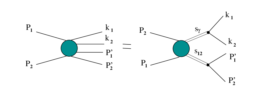
Figure 1: Choice of kinematical variables for the process $N_{1}(P_{1})+N_{2}(P_{2})\to N_{1}^{\prime}(P_{1}^{\prime})+N_{2}^{\prime}(P_{2}^{\prime})+e^{+}(k_{1})+e^{-}(k_{2})$.

The 4-momenta of initial ($P_{1},P_{2}$) and final ($P_{1}^{\prime},P_{2}^{\prime}$) nucleons are $P=(E_{\bf P},{\bf P})$ with $E_{\bf P}=\sqrt{m^{2}+{\bf P}^{2}}$, an analogous notation is used for the lepton momenta $k_{1,2}$; $m$ denotes the nucleon mass, while the electron mass can be neglected for the present kinematics. The invariant mass of two particles is hereafter denoted as $s$ with $s=(P_{1}+P_{2})^{2}$; along with this notation for the invariant mass of the virtual photon throughout the paper we also use the more familiar notation $q^{2}$ with $q^{2}\equiv s_{\gamma}$. As seen from (3), the cross section Eq. (2) is determined by eight independent kinematical variables, the actual choice of which depends upon the specific goals of the considered problem. In the present paper we are mainly interested in studying the invariant mass distribution of the produced electrons and positrons. For this sake it is convenient to choose the kinematics with two invariants, $s_{\gamma}=(k_{1}+k_{2})^{2}$ and $s_{12}=(P_{1}^{\prime}+P_{2}^{\prime})^{2}$, and three solid angles, $d\Omega_{\gamma}^{*}$, $d\Omega_{12}^{*}$ and $d\Omega_{\pm}^{*}$. This corresponds to creation of two intermediate particles with invariant masses $\sqrt{s_{\gamma}}$ and $\sqrt{s_{12}}$ with their subsequent decay into two final nucleons and two leptons, respectively, as depicted in Fig. 1. For each pair, the kinematical variables will be defined in the corresponding two-particle center-of-mass (CM) system. This can be achieved, e.g., by inserting in Eq. (3) the identities

$$1 = \int ds_{\gamma}\ d^{4}P_{\gamma}\ \delta(P_{\gamma}^{2}-s_{\gamma})\ \delta^{(4)}(P_{\gamma}-k_{1}-k_{2}),$$ (4)

$$1 = \int ds_{12}\ d^{4}P_{12}\ \delta(P_{12}^{2}-s_{12})\delta^{(4)}(P_{12}-P_{1}^{\prime}-P_{2}^{\prime})$$ (5)

and rearranging terms in Eq. (3) to separate the invariant phase space volumes for the ”decays” with $P_{\gamma}=k_{1}+k_{2}$ and $P_{12}=P_{1}^{\prime}+P_{2}^{\prime}$, see Fig. 1. With these conventions we arrive at

$$d^{8}\sigma = \frac{1}{2\sqrt{\lambda(s,m^{2},m^{2})}}\frac{1}{(2\pi)^{8}}\frac{1}{4}\sum\limits_{spins}\,|T|^{2}\,\frac{1}{n!}ds_{12}ds_{\gamma}$$

$$\times R_{2}(P_{\gamma}\to k_{1}+k_{2})\ R_{2}(P_{12}\to P_{1}^{\prime}+P_{2}^{\prime})\ R_{2}(P_{1}+P_{2}\to P_{\gamma}+P_{12}),$$

where the two-body invariant phase space volume $R_{2}$ is defined as

$$R_{2}(a+b\to c+d)=d^{4}P_{c}\ d^{4}P_{d}\ \delta^{(4)}(P_{a}+P_{b}-P_{c}-P_{d})\ \delta(P_{c}^{2}-m_{c}^{2})\ \delta(P_{d}^{2}-m_{d}^{2}).$$ (7)

II.2 Leptonic tensor

In the lowest order of the electromagnetic coupling (one-photon approximation) the di-electron production process is considered as decay of a virtual photon produced in strong and electromagnetic $NN$ interactions from different elementary reactions, e.g., bremsstrahlung, Dalitz decay, vector meson decay etc. brat . For such a process the general expression for the invariant amplitude squared reads

$$|T|^{2}=W_{\mu\nu}\,\frac{e^{4}}{q^{4}}l^{\mu\nu},$$ (8)

where the momentum $P_{\gamma}$ of the virtual photon is denoted as $q\equiv P_{\gamma}=(k_{1}+k_{2})$; $e$ is the elementary charge. The purely electromagnetic decay vertex of the virtual photon is determined by the leptonic tensor $l^{\mu\nu}=\sum\limits_{spins}j^{\mu}j^{\nu}$ with the current $j^{\mu}=\bar{u}(k_{1},s_{1})\ \gamma^{\mu}v(k_{2},s_{2})$, where $\bar{u}$ and $v$ are the corresponding Dirac wave functions for the outgoing electron and positron. For unpolarized di-electrons the leptonic tensor reads explicitly

$$l_{\mu\nu}=4\left(k_{1\mu}k_{2\nu}+k_{1\nu}k_{2\mu}-g_{\mu\nu}(k_{1}\cdot k_{2})\right).$$ (9)

The electromagnetic hadronic current $J_{\mu}$ and the hadronic tensor $W_{\mu\nu}=\sum\limits_{spins}J_{\mu}J_{\nu}^{+}$, besides the electromagnetic interaction, also involve the strong interaction between the interacting nucleons and, consequently, are of a more complicate nature than $j_{\mu}$ and $l_{\mu\nu}$. In virtue of gauge invariance the electromagnetic tensors obey $q_{\mu}l^{\mu\nu}=q_{\nu}l^{\mu\nu}=q^{\nu}W_{\mu\nu}=q^{\nu}W_{\mu\nu}=0$, and one can omit in $l^{\mu\nu}$ all terms proportional to $q_{\mu}$ and $q_{\nu}$ and write

$${l}_{\mu\nu}=-2(4k_{1\mu}k_{1\nu}+s_{\gamma}g_{\mu\nu}).$$ (10)

It is evident that the leptonic tensor depends solely upon the kinematical variables connected with the virtual photon vertex (see Fig. 1) and is independent of the variables determining the nucleon-nucleon interaction. This implies that, due to Lorentz invariance of both the amplitude Eq. (8) and the corresponding phase space volume $R_{2}(P_{\gamma}\to k_{1}+k_{2})$, one can carry out the integration over the leptonic variables in any system of reference. The integration is particularly simple in the CM of the leptonic pair, where ${\bf q}=0$, $R_{2}=\sqrt{\lambda(s_{\gamma},\mu_{e}^{2},\mu_{e}^{2})}/8s_{\gamma}\ d\Omega_{\pm}$ and all the time like components of $l_{\mu\nu}$ vanish. One obtains

$$\int d\Omega_{\pm}^{*}W_{\mu\nu}\frac{e^{4}}{q^{4}}l^{\mu\nu}=-\frac{16\pi e^{4}}{3}\frac{J_{\mu}J^{+\mu}}{s_{\gamma}}.$$ (11)

The remaining integrals can be computed by evaluating each differential volume $R_{2}$ also in the corresponding CM system. All together we obtain

$$\frac{d\sigma}{ds_{\gamma}}=-\frac{\alpha_{em}^{2}}{12ss_{\gamma}(4\pi)^{5}}\int ds_{12}d\Omega_{\gamma}^{*}d\Omega_{12}^{*}\sqrt{\displaystyle\frac{\lambda(s,s_{\gamma},s_{12})\lambda(s_{12},m^{2},m^{2})}{s_{12}^{2}\lambda(s,m^{2},m^{2})}}\sum\limits_{spins}J_{\mu}J^{+\mu},$$ (12)

where $d\Omega_{\gamma}^{*}$ and $d\Omega_{12}^{*}$ are defined in the CM of initial and final nucleons, respectively; $\alpha_{em}$ stands for the electromagnetic fine structure constant.

II.3 Lagrangians and parameters

The covariant hadronic current $J_{\mu}$ is evaluated within a meson-nucleon theory based on effective interaction Lagrangians which consist on two parts, describing the strong and electromagnetic interaction. In our approach, the strong interaction among nucleons is mediated by four exchange mesons: scalar ($\sigma$), pseudoscalar-isovector ($\pi$), and neutral vector ($\omega$) and vector-isovector ($\rho$) mesons mosel_calc ; ourOmega ; ourPhi ; scyam_lagr ; bonncd ; chung . We adopt the nucleon-nucleon-meson (NNM) interaction terms

$${\cal L}_{NN\sigma} = g_{\sigma}\bar{N}N\it\Phi_{\sigma},$$ (13)

$${\cal L}_{NN\pi} = -\frac{f_{NN\pi}}{m_{\pi}}\bar{N}\gamma_{5}\gamma^{\mu}\partial_{\mu}({{\mathchar 28956\relax}{\mathchar 28680\relax}_{\pi}})N,$$ (14)

$${\cal L}_{NN\rho} = -g_{NN\rho}\left(\bar{N}\gamma_{\mu}{{\mathchar 28956\relax}}N{{\mathchar 28680\relax}_{\rho}}^{\mu}-\frac{\kappa_{\rho}}{2m}\bar{N}\sigma_{\mu\nu}{{\mathchar 28956\relax}}N\partial^{\nu}{{\mathchar 28680\relax}_{\rho}}^{\mu}\right),$$ (15)

$${\cal L}_{NN\omega} = -g_{NN\omega}\left(\bar{N}\gamma_{\mu}N{\it\Phi}_{\omega}^{\mu}-\frac{\kappa_{\omega}}{2m}\bar{N}\sigma_{\mu\nu}N\partial^{\nu}\it\Phi_{\omega}^{\mu}\right),$$ (16)

where $N$ and $\it\Phi_{M}$ denote the nucleon and meson fields, respectively, and bold face letters stand for isovectors. All couplings with off-mass shell particles are dressed by monopole form factors $F_{M}=\left(\Lambda^{2}_{M}-\mu_{M}^{2}\right)/\left(\Lambda^{2}_{M}-k^{2}_{M}\right)$, where $k^{2}_{M}$ is the 4-momentum of a virtual particle with mass $\mu_{M}$. The effective parameters are adjusted to experimental data on $NN$ scattering. At low energies (below the pion threshold) these parameters are rather well known and can be taken from iterated ${\cal T}$ matrix fits of experimentally known elastic phase shifts bonncd . At intermediate energies, say in the interval 1 - 3 $GeV$, it turns out that the pure tree level description basing on the above interactions is not able to reproduce equally well the energy dependence of the data mosel_calc ; ikh_model . Therefore, following mosel_calc ; ikh_model , we take into account an energy dependence of the effective couplings

$$g_{NNM}\to g_{NNM}(s)=g_{0}{\rm e}^{-l\sqrt{s}}.$$ (17)

In what follows we employ the parameters $l,g_{0}$ and $\Lambda_{M}$ from mosel_calc which assure a good tree level description of the elastic $NN\to NN$, $NN\to N\Delta$ and inelastic $NN\to NN\pi$ reactions at intermediate energies. Note that problems with double counting of the $\Delta$ degrees of freedom are avoided in such an prescription.

II.4 Nucleon form factors and gauge invariance

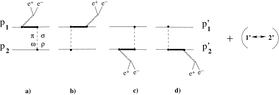
Figure 2: Bremsstrahlung diagrams for the process $N_{1}+N_{2}\to N_{1}^{\prime}+N_{2}^{\prime}+e^{+}e^{-}$ in the one-photon and one-boson exchange approximation (thick lines denote propagators of either nucleons or baryon resonances).

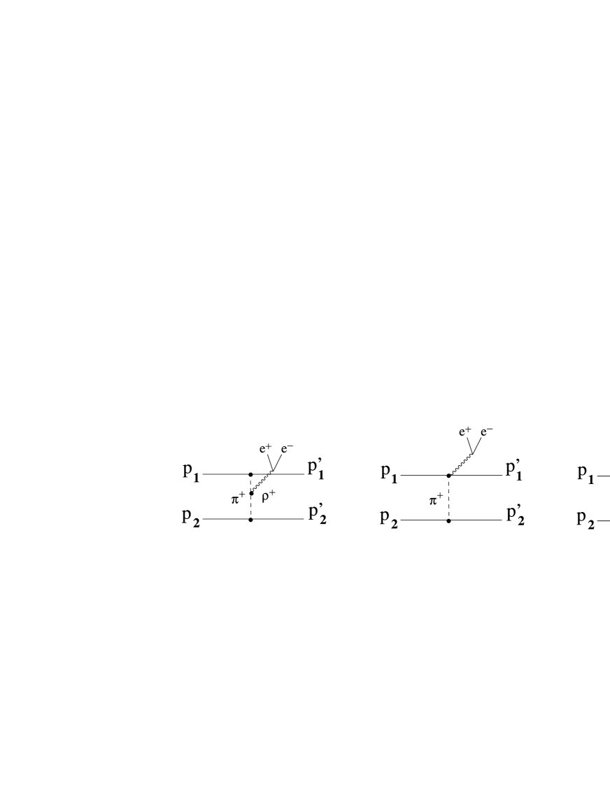
.                   a) b) c)                   .

Figure 3: Contribution of meson exchange currents (a) and seagull terms (b, c) to the process $N_{1}+N_{2}\to N_{1}^{\prime}+N_{2}^{\prime}+e^{+}e^{-}$, where $N_{1}$ and $N_{2}^{\prime}$ stand for protons and $N_{2}$ and $N_{1}^{\prime}$ denote neutrons.

The form of the cross section Eq. (12) bases essentially on the gauge invariance of hadronic and leptonic tensors. This implies that in elaborating models for the reaction (1) with effective Lagrangians particular attention must be devoted to the gauge invariance of the computed currents. In our approach, i.e., in the one-boson exchange approximation (OBE) for the strong $NN$ interaction and one-photon exchange for the electromagnetic production of $e^{+}e^{-}$, the current $J_{\mu}$ is determined by diagrams of two types: (i) the ones which describe the creation of a virtual photon with $q^{2}>0$ as pure nucleon bremsstrahlung as depicted in Fig. 2 and 3b, c, and (ii) in case of exchange of charged mesons, emission of a virtual $\gamma^{*}$ from internal meson lines, see Fig. 3a. For these diagrams the gauge invariance is tightly connected with the two-body Ward-Takahashi (WT) identity (see origwt ; wt1 ; wt2 ; wtTjon and further references therein quoted)

$$q_{\mu}\Gamma^{\mu}(p^{\prime},p)=\frac{e(1+\tau_{3})}{2}\left(S^{-1}(p^{\prime})-S^{-1}(p)\right),$$ (18)

where $\Gamma^{\mu}$ is the electromagnetic vertex and $S(p)$ is the (full) propagator of the particle. It is straightforward to show that, if (18) is to be fulfilled, then pairwise two diagrams with exchange of neutral mesons and pre-emission and post-emission of $\gamma^{*}$ (cf.  Fig. 2b)) cancel each other, hence ensuring $q^{\mu}J_{\mu}=0$, i.e., current conservation (see vmd_ff ). This is also true even after dressing the vertices with phenomenological form factors. However, in case of charged meson exchange the WT identity is not any more automatically fulfilled. This is because the nucleon momenta are interchanged and, consequently, the ”right” and ”left” internal nucleon propagators are defined for different momenta of the exchanged meson. For instance, the contribution to $q^{\mu}J_{\mu}$ from the bremsstrahlung diagrams Fig. 2a) and 2d) reads

$$\bar{u}(P_{1}^{\prime})\Gamma_{NNM}S\left(P_{1}-q\right)\left[S^{-1}\left(P_{1}-q\right)-S^{-1}(P_{1})\right]u(P_{1})\frac{i}{\left(k_{1}^{2}-\mu_{M}^{2}\right)}\bar{u}(P_{2}^{\prime})\Gamma_{NNM}u(P_{1})+$$

$$\bar{u}(P_{1}^{\prime})\Gamma_{NNM}u(P_{1})\frac{i}{\left(k_{2}^{2}-\mu_{M}^{2}\right)}\bar{u}(P_{2}^{\prime})\left[S^{-1}\left(P_{2}^{\prime}\right)-S^{-1}(P_{2}^{\prime}+q)\right]S\left(P_{2}^{\prime}+q\right)\Gamma_{NNM}u(P_{2})$$

$$=\bar{u}(P_{1}^{\prime})\Gamma_{NNM}u(P_{1})\left[\frac{i}{\left(k_{1}^{2}-\mu_{M}^{2}\right)}-\frac{i}{\left(k_{2}^{2}-\mu_{M}^{2}\right)}\right]\bar{u}(P_{2}^{\prime})\Gamma_{NNM}u(P_{2}),$$ (19)

where $k_{1}=P_{2}^{\prime}-P_{2}$ , $k_{2}=P_{1}^{\prime}-P_{1}$, $S^{-1}\left(P_{1}\right)u(P_{1})=0$ and $\bar{u}(P_{2}^{\prime})S^{-1}\left(P_{2}^{\prime}\right)=0$. In fact, $q_{\mu}J^{\mu}\neq 0$ follows. In order to restore the gauge invariance on this level one must consider additional diagrams with emission of the virtual photon by the charged meson exchange as depicted in Fig. 3a. Then it is easy to show that the contribution from this diagram exactly compensates the non-zero part (19), and thus gauge invariance is restored. This holds for bar $NNM$ vertices without cut-off form factors. Inclusion of additional form factors again leads to non-conserved currents. There are several prescriptions of how to preserve gauge invariance within effective theories with cut-off form factors wtTjon ; mosel_calc ; vmd_ff ; gross . The main idea of these prescriptions is to include the cut-off form factors into WT identity explicitly and to consider the new relations as the WT identity for the full propagators. For instance, Refs vmd_ff ; gross suggest to interpret the cut-off form factors as an effective account of the self-energy corrections and to present the full propagators, entering the WT identity (18), as the bare ones multiplied from the both ends of the propagator line by phenomenological cut-off functions. Formally, all the Feynman rules to calculate ladder diagrams as exhibited in Fig. 2 remain unchanged, while in calculation of diagram types as depicted in Fig. 3a the meson-nucleon vertex must be multiplied by the square of the cut-off form factor $F_{MNN}^{2}(k)$; consequently a factor $F_{MNN}^{-1}(k)$ must be included into the effective electromagnetic $MM\gamma$ vertex. In the simplest case the bare mesonic vertex $\Gamma_{\mu}^{M}=\left(k_{1\mu}+k_{2\mu}\right)$ receives an additional factor schafer ; mathiot

$$F_{add}=1-\frac{k_{1}^{2}-\mu_{M}^{2}}{\Lambda_{m}^{2}-k_{2}^{2}}-\frac{k_{2}^{2}-\mu_{M}^{2}}{\Lambda_{M}^{2}-k_{1}^{2}}$$ (20)

becoming

$$\Gamma_{\mu}^{\gamma M}=\left(k_{1\mu}+k_{2\mu}\right)\frac{\left(\Lambda_{M}^{2}-k_{1}^{2}\right)}{\left(\Lambda_{M}^{2}-\mu_{M}^{2}\right)}\frac{\left(\Lambda_{M}^{2}-k_{2}^{2}\right)}{\left(\Lambda_{M}^{2}-\mu_{M}^{2}\right)}F_{add}.$$ (21)

It can be seen that the ”renormalized” vertex (21) obeys the WT identity for the full, renormalized mesonic propagators. In a more general case, on can add to the vertex (21) any divergenceless term, which obviously does not change the WT identity. Often it is convenient to display in the mesonic vertices some terms which assure the WT identity and the divergenceless part explicitly, in which case the corresponding vertex reads as (see also Ref. wtTjon )

$$\Gamma_{\mu}^{\gamma M}=\frac{q_{\mu}}{q^{2}}\left(\Delta^{-1}(k_{1}^{2})-\Delta^{-1}(k_{2}^{2})\right)+B(k_{1},k_{2})\left[(k_{1\mu}+k_{2\mu})-q_{\mu}\frac{q\cdot(k_{1}+k_{2})}{q^{2}}\right],$$ (22)

where $\Delta(k^{2})$ denotes the scalar propagator and $B(k_{1},k_{2})$ is an arbitrary scalar function. In accordance with gross , the meson propagators are to be multiplied by cut-off form factors at both ends of their lines in the diagram Fig. 3a, resulting in

$$\Delta(k^{2})=\frac{F_{MNN}^{2}(k^{2})}{k^{2}-\mu_{M}^{2}}.$$ (23)

Note that the above prescriptions for restoration of the gauge invariance in $pn$ collisions are valid only if the effective meson-nucleon interaction vertices do not depend on the momentum $k$ of the exchanged meson. This is the case for pseudo-scalar $\pi NN$ coupling. Instead, if the pseudo-vector $\pi NN$ coupling (14) is chosen then the Fourier transformed four divergence of the currents corresponding to diagrams Fig. 2 contains an additional $k$ dependence from the derivatives in the $\pi NN$ vertex (cf. Eq. (16)) yielding

$$\!\!\!\!\!\!\!\!q_{\mu}J^{\mu}\sim\bar{u}(p_{1}^{\prime})\gamma_{5}\hat{k}_{1}u(p_{1})\Delta(k_{1}^{2})\bar{u}(p_{2}^{\prime})\gamma_{5}\hat{k}_{1}u(p_{2})-\bar{u}(p_{1}^{\prime})\gamma_{5}\hat{k}_{2}u(p_{1})\Delta(k_{2}^{2})\bar{u}(p_{2}^{\prime})\gamma_{5}\hat{k}_{2}u(p_{2}).$$ (24)

The contribution of the diagram Fig. 3a with the mesonic vertex (21) or (22) to $q^{\mu}J_{\mu}$ reads very similar to (24) but in each term both momenta, $\hat{k}_{1}$ and $\hat{k}_{2}$ enter, and consequently, the gauge invariance can not be completely restored. Within an effective meson nucleon theory with interaction Lagrangians depending on derivatives, the gauge invariant coupling with photons is introduced by replacing partial derivatives, including the $NNM$ vertices, by a gauge covariant form (minimal coupling). Such a procedure generates another kind of Feynman diagrams with contact terms, i.e., vertices with four lines, known also as Kroll-Rudermann KR or seagull like diagrams, see Figs. 3b and c. We include therefore in our calculations these diagrams and the corresponding interaction Lagrangian

$${\cal L}_{NN\pi\gamma}=-\frac{\hat{e}f_{NN\pi}}{m_{\pi}}\bar{N}\gamma_{5}\gamma^{\mu}A_{\mu}({{\mathchar 28956\relax}{\mathchar 28680\relax}_{\pi}})N$$ (25)

with 4-potential $A_{\mu}$ and charge operator $\hat{e}$ of the pion. Gauge invariance is henceforth ensured. The contact term contributions become particularly important near the kinematical limits.

All electromagnetic $NN\gamma$ vertices corresponding to the interaction Lagrangian

$${\cal L}^{em}_{NN\gamma}=-e\left(\bar{N}\gamma_{\mu}N\right)A^{\mu}+e\kappa\bar{N}\left(\frac{\sigma_{\mu\nu}}{4m}{\cal F}^{\mu\nu}\right)N$$ (26)

with the field strength tensor ${\cal F}^{\nu\mu}=\partial_{\nu}A^{\mu}-\partial_{\mu}A^{\nu}$, and $\kappa$ as the anomalous magnetic moment of the nucleon ($\kappa=1.793$ for protons and $\kappa=-1.913$ for neutrons), should also be dressed by form factors. This means that at least two form factors are needed to describe electron scattering from on-mass shell nucleons.

In the more general case of off-mass shell nucleons even eight terms, satisfying the necessary symmetry and gauge invariance requirements, with eight scalar form factors contribute to the $NN\gamma$ vertex. At $q^{2}<0$ and low nucleon virtuality ($P^{2}\sim m^{2}$) it is still possible to restrict this set to two effective form factors to describe electron scattering from off-mass shell nucleons (e.g., in $A(e,e^{\prime}p)$ reactions) by modifying (kinematically) the $NN\gamma$ vertex to satisfy gauge invariance (see for details, deForest and further references therein quoted). Unfortunately, for $q^{2}>0$ information about the electromagnetic form factors can be obtained directly only at $q^{2}>4m^{2}$ (e.g., from proton-antiproton annihilation into an electron-positron pair or the inverse reaction), while the region $0<q^{2}<4m^{2}$ remains unaccessible in an on-mass shell process. This is just the region which includes vector meson production and thus, could provide some tests of the validity of the vector meson dominance (VMD) sacurai model for the electromagnetic coupling to off-mass shell nucleons.

Various models have been elaborated to calculate the form factors in the time like region below the $N\bar{N}$ threshold (see, e.g., wtTjon ; vmd_ff ; vmd_ff1 ) which basically treat the electromagnetic vertex within an effective meson-nucleon theory in terms of photon couplings directly to bare nucleons superimposed to the coupling to the meson cloud surrounding the nucleon. Besides, one can apply an analytical continuation of form factors based on VMD sacurai which suggests that the photon first converts into a vector meson which then couples to hadrons. This model provides a successful description of the on-mass shell pion form factor. For nucleons, VMD predicts a strong resonance behavior of the time like form factors in the neighborhood of vector meson pole masses. However, the dipole like behavior of the space like nucleon form factor persuades us that VMD is too strong a restriction. In principle, the original conjecture of VMD could be augmented by introducing heavier vector mesons (see, e.g., hohler ) into the parametrization of the nucleon form factor.

The eight independent form factors can be defined in terms of positive and negative energy projection operators as wtTjon

$$\Gamma_{\mu}\left(P^{\prime},P\right)=e\sum\limits_{\rho_{1}=\pm,\ \rho_{2}=\pm}\Lambda^{\rho_{1}}\left[F_{1}^{\rho_{1},\rho_{2}}\gamma_{m}u+\frac{i\sigma_{\mu\nu}q^{\nu}}{2m}F_{2}^{\rho_{1},\rho_{2}}+q_{\mu}F_{3}^{\rho_{1},\rho_{2}}\right]\Lambda^{\rho_{2}},$$ (27)

where the third form factor $F_{3}^{\rho_{1},\rho_{2}}$ is not an independent one, but is connected with $F_{12}^{\rho_{1},\rho_{2}}$ via the WT identity. The positive ($\rho=+$) and negative ($\rho=-$) energy projection operators are denoted as $\Lambda^{\pm}$ respectively. For the half off-mass shell nucleons only four terms contribute to the electromagnetic vertex. As mentioned above, in the time like region below the $N\bar{N}$ threshold these form factors are to be computed as loop corrections to the bare electromagnetic vertex wtTjon and/or as analytical continuation of the VMD prediction. Microscopical calculations vmd_ff show that the electromagnetic form factors are rather sensitive to model assumptions in the region of vector meson pole masses. At low energies they depend weakly on $q^{2}$ and can be effectively absorbed into the effective parameters of the $NN\gamma$ Lagrangian mosel_calc ; pascScholten .

In the present paper we are primarily interested in di-electron production at intermediate energies with the mass distributions sufficiently far from the vector meson pole masses so that, following mosel_calc ; pascScholten , we merely put $F_{1}=1$ and instead of $F_{2}$ we use the anomalous magnetic moment of the corresponding nucleon, i.e., we use the Lagrangian (26). However, for purely methodological sakes, we also present some results on di-electron production at higher energies, where the $e^{+}e^{-}$ invariant mass covers the $\rho$ and $\omega$ pole masses to evidence effects of the present VMD implementation.

II.5 $\Delta$ isobar

Intermediate baryon resonances play an important role in di-electron production in $NN$ collisions fuchs ; ernst ; nakayama ; lutzNew ; kapusta ; mosel_calc ; ikh_model ; schafer ; brat . At intermediate energies the main contribution to the cross section stems from the $\Delta$ isobar mosel_calc . Since the isospin of the $\Delta$ is $3/2$ only the isovector mesons $\pi$ and $\rho$ couple to nucleons and $\Delta$. The form of the effective $\Delta N$ interaction was thoroughly investigated in literature in connection with $NN$ scattering bonncd ; holinde ; weise , pion photo- and electroproduction pascQuant ; photo ; davidson ; elctro ; lenske . The effective Lagrangians of the $N\Delta M$ interactions read holinde ; weise ; pascQuant )

$${\cal L}_{\Delta N\pi}=\frac{f_{\Delta N\pi}}{\mu_{\pi}}\left[\bar{\Psi}_{\Delta}^{\alpha}\ {\bf T}\ \partial_{\alpha}{\mathchar 28680\relax}_{\pi}N\right]+h.c.,$$ (28)

$${\cal L}_{\Delta N\rho}=\frac{if_{\Delta N\rho}}{\mu_{\rho}}\left[\bar{\Psi}_{\Delta\,\alpha}{\bf T}\left\{\partial^{\beta}{\mathchar 28680\relax}_{\rho}^{\alpha}-\partial^{\alpha}{\mathchar 28680\relax}_{\rho}^{\beta}\right\}\gamma_{\beta}\gamma_{5}N\right]+h.c.$$ (29)

with $f_{\Delta N\pi}=2.13\ GeV$ and $f_{\Delta N\rho}=7.14\ GeV$ schafer . The couplings are dressed by cut-off form factors

$$F^{N\Delta M}=\left[\frac{\Lambda_{N\Delta M}^{2}-\mu_{M}^{2}}{\Lambda_{N\Delta M}^{2}-k^{2}}\right]^{2},$$ (30)

where $\Lambda_{N\Delta\pi}=1.421\ GeV$ and $\Lambda_{N\Delta\rho}=2.273\ GeV$ schafer . The symbol ${\bf T}$ stands for the isospin transition matrix (see Appendix A), $\Psi_{\Delta}$ denotes the field describing the $\Delta$. Usually particles with higher spins ($s>1$) are treated within the Rarita-Schwinger formalism in accordance with which the $\Delta$ field is a rank-1 tensor (obeying the Klein-Gordon equation) each component of which is a 4-spinor satisfying the Dirac equation as well. To reduce the number of redundant degrees of freedom the Rarita-Schwinger field satisfies also a number of additional subsidiary conditions (cf. fronsdal ). Nevertheless, such a field does not uniquely determine the properties of spin-$3/2$ particles. It is known that an arbitrary field of rank 1 provides a basis for a reducible representation of the Lorentz group, which can be decomposed into two irreducible representations corresponding to spins $s=1$ and $s=0$ of the vector field. Correspondingly, an arbitrary solution of field equations for $\Psi_{\Delta}$ will be related to spins $s=3/2$ and $s=1/2$. In order to eliminate the part corresponding to $s=1/2$ one usually considers spin projection operators fronsdal acting on an arbitrary solution of the field equations which ensure the uniqueness of the description of particles with high spins via

$$\Psi^{\alpha}_{\Delta}=P_{\frac{3}{2}}^{\alpha\beta}\ \Psi^{\beta},$$ (31)

where $\Psi^{\beta}$ is a solution of the spin-$\frac{3}{2}$ field equations and the spin projection operator is defined as

$$P_{\frac{3}{2}}^{\alpha\beta}(p)=g^{\alpha\beta}-\frac{1}{3}\gamma^{\alpha}\gamma^{\beta}-\frac{2}{3m_{\Delta}^{2}}p^{\alpha}p^{\beta}-\frac{1}{3m_{\Delta}}\left(\gamma^{\alpha}p^{\beta}-\gamma^{\beta}p^{\alpha}\right).$$ (32)

Then the propagator for the high-spin particles is constructed in a fully analogous way with the case $s=1/2$. Remaind that formally the propagator of a Dirac particle with $s=1/2$ can be expressed as a product of a scalar propagator multiplied by the positive energy projection operator $\Lambda^{+}=\hat{p}+m$ evaluated at $p^{2}\neq m^{2}$. For the Rarita-Schwinger propagator, in order to ensure the propagation of degrees of freedom with $s=3/2$, one usually includes also the spin projection operator $P_{\frac{3}{2}}$ to obtain

$$S_{\Delta}^{\alpha\beta}(p)=-\frac{i\left(\hat{p}+m_{\Delta}\right)}{p^{2}-m_{\Delta}^{2}}\ P_{\frac{3}{2}}^{\alpha\beta}(p).$$ (33)

This propagator is discussed in the literature will ; post ; titovprop ; tjonprop with respect to the fact that for free particles the positive energy projection operator $\Lambda^{+}(p)$ commutes with the spin projection operator $P_{\frac{3}{2}}^{\alpha\beta}(P)$, which is not the case for off-mass shell operators. The adopted order of their multiplication is rather a convention than a rule. Another source of ambiguity is the convention of what to use in (33) as the ”particle mass”, the on-mass shell value $m_{\Delta}$ or the off-mass shell invariant mass $\sqrt{p^{2}}$ tjonprop ; pascScholten . Note that different prescriptions for the propagator differ by corrections of the order $p^{2}-m_{\Delta}^{2}$ which, at intermediate energies, could be absorbed in slight readjustments of the effective parameters. Indeed, changing the order of the operators in (33) we find an almost constant modification of the cross sections over a wide range of kinematic variables.

In our calculations we adopted the prescription of fronsdal ; mosel_calc , i.e., the propagator is taken according to Eq. (33). In addition, to take into account the finite life time of $\Delta$, in the denominator of the scalar part of the propagator, the mass is modified by adding the width, i.e., $m_{\Delta}\to m_{\Delta}-i\Gamma_{\Delta}/2$. For the kinematics considered here the mass of the intermediate $\Delta$ can be rather far from its pole value, so that the width, as a function of $p^{2}_{\Delta}$, is calculated as a sum of partial widths through the one-pion ($\Delta\to N\pi$) and two-pion ($\Delta\to N\rho\to N2\pi$) decay channels shyamwidts .

The general form of the $\Delta N\gamma$ coupling satisfying the gauge invariance can be written as davidson ; feuster ; pascTjon ; pascScholten

$${\cal L}_{\Delta N\gamma} = -i\frac{eg_{1}}{2m}\bar{\Psi}^{\alpha}\Theta_{\alpha\mu}(z_{1})\gamma_{\nu}\gamma_{5}{\bf T}_{3}\psi{\cal F}^{\nu\mu}-\frac{eg_{2}}{4m^{2}}\bar{\Psi}^{\alpha}\Theta_{\alpha\mu}(z_{2})\gamma_{5}{\bf T}_{3}\left(\partial_{\nu}\psi\right){\cal F}^{\nu\mu}$$ (34)

$$-\frac{eg_{3}}{4m^{2}}\bar{\Psi}^{\alpha}\Theta_{\alpha\mu}(z_{3})\gamma_{5}{\bf T}_{3}\psi\partial_{\nu}{\cal F}^{\nu\mu}+h.c.,$$

$$\Theta_{\alpha\mu}(z) = g_{\alpha\mu}+[z+\frac{1}{2}(1+4z)A]\gamma_{\alpha}\gamma_{\mu},$$ (35)

where $A$ is a constant reflecting the invariance of the free $\Delta$ Lagrangian with respect to point transformations rarita . Since observables must not depend on this parameter, $A$ is arbitrary. According to common practice one puts $A=-1$. The other parameter, $z$, is also connected with point transformations, however it is a characteristic of the off-mass shell $\Delta$ resonance and remains unconstrained. The meaning of this parameter is that every coupling to a spin-$3/2$ field contains also contributions from couplings with spin-$1/2$ components. Some times $z$ is called the off-mass shell parameter. Investigations of the role of the off-mass shell quantity, treated as a free parameter, in different observables related to the $\Delta$ show feuster ; davidson that inclusion of $z$ into the calculations requires a slight readjustment of the effective parameters $g_{i}$, which are also free parameters. This means that the parameter $z$ and the effective couplings $g_{i}$ must be simultaneously adjusted to given observables. A thorough study of the role of couplings to spin-$1/2$ particles pascQuant ; pascScholten has shown that the dependence on $z$ is rather weak, making the off-mass shell parameter redundant (see also discussion in mosel_calc ). Basing on this observation, we neglect the off-mass shell parameter by merely putting $\Theta_{\alpha\mu}(z)=g_{\alpha\mu}$. The coupling constants $g_{i}$ are taken as in mosel_calc , i.e., $g_{1}=5.416$, $g_{2}=6.612$ and $g_{3}=7.0$.

II.6 Results for $NN\to NN$

As mentioned above our effective parameters have been fixed in such a way as to reproduce reasonably well the results of the study mosel_calc performed to explain the DLS data DLS at low energies. The OBE parameters (listed in Table 1) and their energy dependence have been taken as in Ref. mosel_calc . Figures 4 and 5 show results of our calculations of the mass distribution of di-electrons in $pp$ and $pn$ collisions at two values of the kinetic energy, $1.04\ GeV$ and $2.09\ GeV$, corresponding to those considered in mosel_calc . The dotted lines depict the contribution of pure bremsstrahlung processes from nucleon lines, i.e., di-electrons are produced solely due to nucleon-nucleon interaction via the one-boson-exchange potential. In our actual calculations we include four exchange mesons, $\pi$, $\sigma$, $\rho$ and $\omega$ mesons supplemented by a ”counter” term simulating a heavy axial vector-isovector meson, with the goal to cancel singularities of the pion potential at the origin mosel_calc .

The dashed lines in Figs. 4 and 5 depict the contributions of the $\Delta$ isobar within the same OBE potential. The solid lines represent the total cross section including all interferences. It can be seen that for $pp$ collisions almost in the whole kinematical range the $\Delta$ contribution dominates. Near the kinematical limits the nucleon contribution becomes comparable with $\Delta$ contributions. At smaller invariant masses, the $N$ and $\Delta$ contributions interfere constructively, while near the kinematical limit and at beam energy $2.09\>GeV$ the interference pattern in $pp$ reactions is just so that the total cross section resembles the $N$ or $\Delta$ contributions individually. Another observation is the fact that, due to isospin factors the cross section in $pn$ reactions is systematically larger than in $pp$ reactions. These results are in agreement with mosel_calc . In $pn$ collisions the inclusion of the contact terms amplifies the contribution of pure nucleon diagrams.

After adjusting the model parameters we proceed and present in Figs. 6 and 7 results at energies envisaged in the approved HADES proposal HADES for $pp$ and $pn$ processes. It is seen that, except for the absolute values, the behavior of the cross section and the relative contributions of $\Delta$ isobars and pure nucleon bremsstrahlung basically does not change with energy. However, as seen from these figures, the kinematical range of the di-electron mass becomes essentially larger covering also the region of vector meson production, i.e., $\rho$ and $\omega$, which have been not yet implemented in the calculations. Consequently, at these energies the results presented in Figs. 6 and 7 are to be considered as an estimate of a smooth bremsstrahlung background. Effects of $\rho$ and $\omega$ excitations will be considered in the next subsection.

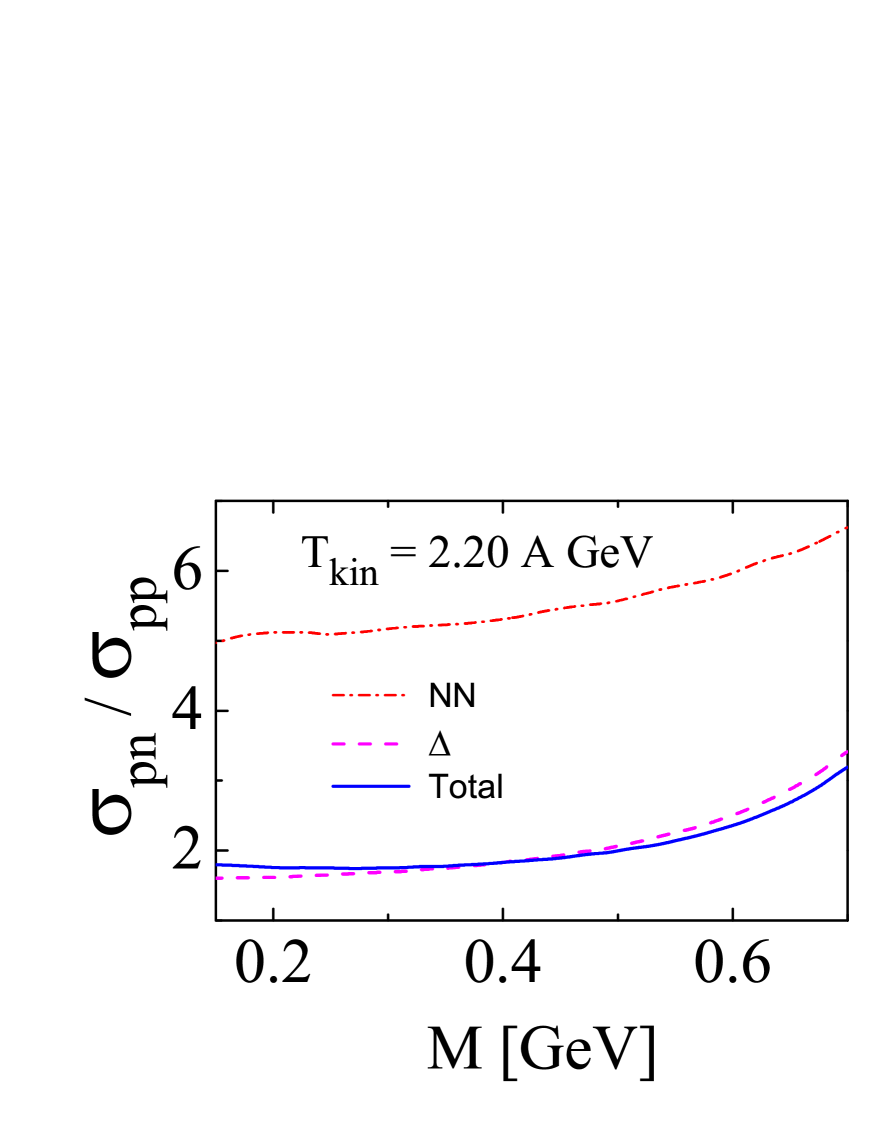
Figure 8: The ratio $\sigma(pn\to pne^{+}e^{-})$ to $\sigma(pp\to ppe^{+}e^{-})$ as a function of the invariant mass at $T_{\rm kin}=2.2\,GeV$. The dot-dashed and dashed curves exhibit results with only nucleon and $\Delta$ contributions, respectively. The ratio of the total cross sections is denoted by the solid line.

In Fig. 8 the isospin effects in $pn$ and $pp$ reactions are quantified. The dot-dashed line illustrates the difference between $pp$ and $pn$ processes in pure nucleon bremsstrahlung, the dashed line reflects the isospin effects for the $\Delta$ contribution, while the full line is the ratio of the total cross sections. Note the nontrivial invariant mass dependence which prohibits the use of simple, constant isospin factors to relate $pp\to pp\>e^{+}e^{-}$ and $pn\to pn\>e^{+}e^{-}$ cross sections.

II.7 VMD effects

As seen in Figs. 6 and 7, at beam energies $T_{kin}>2\>GeV$ the kinematical range of the invariant mass $M$ covers the $\rho$ and $\omega$ pole masses (corresponding to $0.768$ and $0.783\ GeV$, respectively) so that in this region the vector meson nature of the electromagnetic coupling of photons with nucleons can show up. In simple terms, the VMD hypothesis sacurai implies that photons couple to hadrons ($\pi$ mesons, nucleons etc.) solely via intermediate vector mesons, in which case the electromagnetic form factor reads

$$F_{VMD}(q^{2})=\frac{M_{V}^{2}}{M_{V}^{2}-q^{2}}.$$ (36)

Such a behavior of form factors can be obtained in a more rigorous way within an effective meson-nucleon theory, like the one used in the present paper. For this purpose one should consider additionally effective Lagrangians with electromagnetic couplings of the vector mesons (only $\rho$ and $\omega$ in the kinematical region we are interested in) with photons. This procedure is not unique and one should pay attention to avoid double counting of contributions from the Lagrangian with direct $NN\gamma$ coupling. Usually lutzNew ; vmd_ff ; vmd_ff1 ; friman1 the electromagnetic $\gamma\rho$ and $\gamma\omega$ interaction Lagrangians are added to the $NN\gamma$ Lagrangian (26) and are chosen in the form

$${\cal L}^{em}_{\rho(\omega)\gamma}=-\frac{e}{2f_{\rho(\omega)\gamma}}{\cal F}^{\nu\mu}{\cal G^{\rho(\omega)}}_{\nu\mu},$$ (37)

where ${\cal G^{\rho(\omega)}}_{\nu\mu}$ is the field strength tensor of the $\rho\>(\omega)$ meson. Note that the Lagrangian (37) should be considered only together with the Lagrangians (16) and (26), in which case the proton electromagnetic vertex reads

$$\Gamma^{\mu}_{NN\gamma}=\left(\gamma^{\mu}-\displaystyle\frac{q^{\mu}\hat{q}}{q^{2}}\right)F_{1}(q^{2})+\displaystyle\frac{q^{\mu}\hat{q}}{q^{2}}+i\kappa F_{2}(q^{2})\frac{\sigma^{\mu\nu}q_{\nu}}{2m},$$ (38)

where

$$F_{1}(q^{2})=1+\frac{g_{NN\rho}}{f_{\rho\gamma}}\left[\frac{q^{2}}{M_{\rho}^{2}-q^{2}}+\frac{f_{\rho\gamma}}{f_{\omega\gamma}}\frac{g_{NN\omega}}{g_{NN\rho}}\frac{q^{2}}{M_{\omega}^{2}-q^{2}}\right],$$

$$F_{2}(q^{2})=1+\frac{g_{NN\rho}}{f_{\rho\gamma}}\frac{q^{2}}{M_{\rho}^{2}-q^{2}}.$$ (39)

Note that the vertex function (38) obeys the WT identity. The introduced coupling constants can be estimated from VMD like pole fits hohler ; dubnicka ; gari and also from the requirement that at $q_{\mu}\to 0$ one has $F_{1}\to(1+\tau_{3})/2$ (see also wtTjon ; friman1 ). As a result, one can approximately take

$$\frac{g_{NN\rho}}{f_{\rho\gamma}}=\frac{1}{2},\quad\frac{f_{\rho\gamma}}{f_{\omega\gamma}}\frac{g_{NN\omega}}{g_{NN\rho}}=1,$$ (40)

which provides the following form of the form factors

$$F_{1}(q^{2})=1+\frac{1}{2}\left[\frac{q^{2}}{M_{\rho}^{2}-q^{2}}+\frac{q^{2}}{M_{\omega}^{2}-q^{2}}\right],$$ (41)

$$F_{2}(q^{2})=1+\frac{1}{2}\frac{q^{2}}{M_{\rho}^{2}-q^{2}}.$$ (42)

Since both $\rho$ and $\omega$ are not stable the corresponding masses in (41) and (42) receive also imaginary parts, i.e., $M_{V}\to M_{V}-iM_{V}\Gamma_{V}/2$, where $\Gamma_{V}$ is the total decay width of the respective vector meson. In our calculations we take advantage of the fact that a free $\rho$ meson decays mainly into two pions, so that its width, as a function of the invariant mass $q^{2}$, can be calculated within the same effective meson-nucleon theory with the result

$$\Gamma_{\rho}(q^{2})=\Gamma_{\rho}(M_{\rho}^{2})\frac{M_{\rho}^{2}}{q^{2}}\left(\displaystyle\frac{\sqrt{q^{2}-4\mu_{\pi}^{2}}}{\sqrt{M_{\rho}^{2}-4\mu_{\pi}^{2}}}\right)^{3},$$ (43)

where $\Gamma_{\rho}(q^{2}=M_{\rho}^{2})\approx 0.15\ GeV$. The width of the $\omega$ meson in the present calculations has been kept constant $\Gamma_{\omega}=0.03\ GeV$ to simulate the finite resolution HADES (HADES envisages an invariant mass resolution $\Delta M/M\sim 1\%$ holzman ). Note that the VMD model can be recovered if, as usually, one takes $M_{\rho}\approx M_{\omega}=M_{V}$ and $\Gamma_{\rho}\approx\Gamma_{\omega}$.

Some comments are in order here. The VMD hypothesis could be implemented not only via the effective Lagrangians (37), (16) and (26) but also by considering the simplest form for the $\gamma V$ coupling wtTjon ; kroll ; friman2

$${\cal L}_{VMD}=-\frac{eM_{\rho(\omega)}^{2}}{f_{\rho(\omega)\gamma}}\Phi^{\mu}_{\rho(\omega)}A_{\mu}$$ (44)

without the direct term (26). The Lagrangian (44) corresponds better to the original VMD conjecture sacurai since it assumes that the electromagnetic coupling $NN\gamma$ occurs solely via the vector mesons. It is easily seen that if one employs the Lagrangians (16) and (44), e.g., the form factor $F_{1}$ with $M_{\rho}\approx M_{\omega}=M_{V}$ and $\Gamma_{\rho}\approx\Gamma_{\omega}$, the VMD form (41) or (36) could be obtained wtTjon . An inclusion of direct terms, like Eq. (26), will lead to double counting in the corresponding amplitude. Hence, the Lagrangian (44) simultaneously accounts for vector meson production effects near the corresponding pole masses ($M_{\rho}$ and $M_{\omega}$) and for the background (direct) contribution in the whole kinematical range. Consequently a separation of these two kinds of effects is hampered with the VMD Lagrangian taken as in Eq. (44). In our calculations we use the Lagrangians (26) and (37) which allow to distinguish the contribution of direct terms from the vector meson production, i.e., the first term in Eqs. (41) and (42) is referred to as the direct or background contribution, while the second one defines the $\rho$ and $\omega$ meson contribution (see also vmd_ff ).

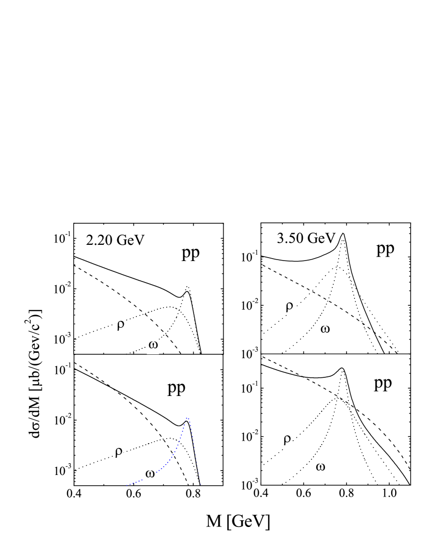
Figure 9: Illustration of the role of the VMD effects for the invariant mass distribution of di-electrons produced in $pp$ reactions. The left and right panels are for initial energies $T_{kin}=2.2\>GeV$ and $T_{kin}=3.5\>GeV$, respectively. In the upper row results are presented for nucleon contributions solely, while in the lower one the total cross sections, including $\Delta$ isobars, are shown. The dashed lines present the background contribution (cf. Fig. 6), dotted lines exhibit the pure VMD effects, i.e., the separate contribution from $\rho$ and $\omega$ mesons. The solid lines illustrate the effects of VMD for the total cross section (bottom panels) and for pure nucleon contributions (i.e., without $\Delta$, top panels).

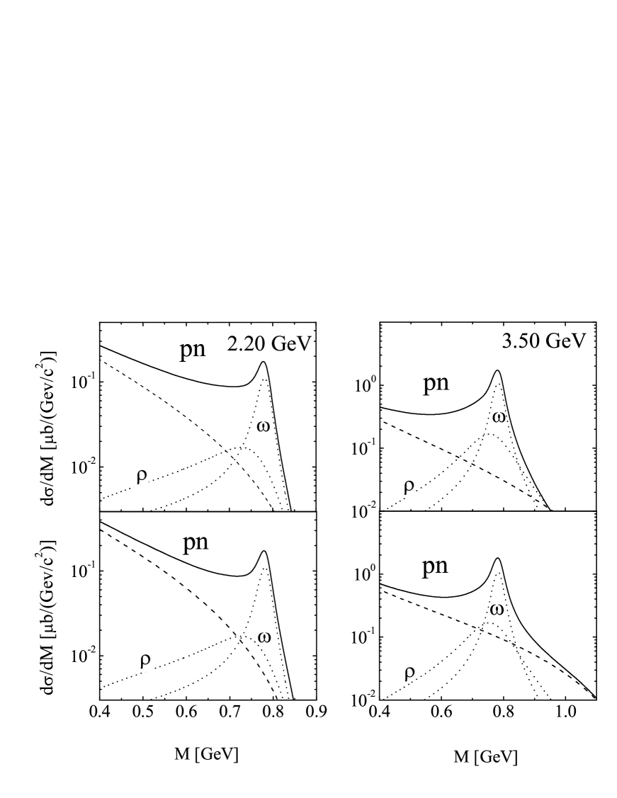
Figure 10: Same as Fig. 9 but for $pn$ reactions.

Figures 9 and 10 illustrate the effects of VMD at two kinetic beam energies, $T_{kin}=2.2\ GeV$ and $T_{kin}=3.5\ GeV$, for $pp$ and $pn$ collisions, respectively. In the upper panels we present VMD effects for the pure nucleon contribution, while in the lower panels the $\Delta$ contribution is included as well. The dashed lines represent the background cross section, i.e., the one calculated with only the first term in Eqs. (41) and (42) (cf. Figs. 6 and 7). The dotted lines have been obtained when only the second ($\rho$) or the third terms ($\omega$) have been taken into account. It is seen that the resonance structure of the $\rho$ contribution is not so pronounced being rather broad, because of its relatively low threshold and because of the mass dependence of its the decay width. Contrarily, the $\omega$ contribution has a rather sharp, resonance like behavior. The relative contribution of $\omega$ and $\rho$ near the pole mass, $M_{0}\sim M_{\omega}\sim M_{\rho}\sim 0.78\ GeV$, is basically governed by the ratio of meson widths squared, $\Gamma_{\omega}^{2}(M_{0})/\Gamma_{\rho}^{2}(M_{0})=0.03^{2}/0.15^{2}$ (remind that we attribute to the $\omega$ meson the actual width of $30\>MeV$ to simulate finite detector resolution).

Here it is worth stressing that within the VMD model the vector mesons are designed to mediate the electromagnetic coupling of photons with nucleons. Consequently, they contribute in the whole kinematical range of the invariant mass and, except the neighborhood of the pole masses, are essentially virtual. This implies that, apart from the intervals near the pole masses, the cross section can not be presented as a two-step process consisting of: (i) production of a vector meson resonance with experimentally known width and with a mass around the $\rho$ and/or $\omega$ mass, (ii) the independent subsequent decay into a di-electron channel (cf. discussion in Ref. knoll ). The di-electron emission within the VMD model is rather a process of production of a virtual vector particle with the quantum numbers of the $\rho$ or/and $\omega$ with subsequent decay into a di-electron (via an intermediate conversion into a virtual photon) which contributes in the whole kinematical range of the di-electron invariant masses. This issue is discussed in some detail in Appendix B.

II.8 Effects of final state interaction

Previous studies of threshold-near vector meson production in $NN$ reactions have shown nakayama ; ourOmega ; titovprop ; titov that the final state interaction (FSI) between nucleons plays an important role. It has been also found that considerable corrections from FSI occur at low values of the energy excess, $\Delta s^{\frac{1}{2}}=\sqrt{s}-2m-M_{V}$, where the relative momentum (excitation energy) of the nucleon pair is small. With increasing energy excess the relative momentum increases too and FSI effects become less important nakayama ; ourOmega .

In reactions of di-electron production the kinematical situation is rather different. As seen from Eq. (12) the invariant mass, $s_{\gamma}$, of the $e^{+}e^{-}$ pair varies from the photon point to a maximum value dictated by kinematics. Similar to the case of on-mass shell vector meson production (cf. Eq. (2.4) in Ref. ourOmega ), in Eq. (12) an integration over the excitation energy $s_{12}$ is to be performed. However, in this case the kinematical range of $s_{12}$ and, consequently, the range of the relative momentum of the nucleon pair is rather different and strongly depends on the value of the di-electron invariant mass. With increasing di-electron mass FSI effects are expected to increase. For instance, the results of Ref. ourOmega indicate that for $pn$ reactions at di-electron mass near the $\omega$ pole mass, FSI effects lead to an increase of the cross section by a factor $\sim 2$, while at lower masses the FSI effects are expected to diminish. However, with increasing di-electron mass, the kinematical range of $s_{12}$ shrinks, so that FSI effects are expected to increase.

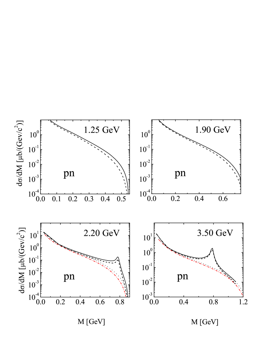
Figure 11: Illustration of the role of FSI effects in the invariant mass distribution of di-electrons produced in $pn$ reactions. The four panels correspond to the initial beam energies $T_{kin}=1.25\ GeV$, $\>1.9\ GeV$, $\>2.2\ GeV$ and $\>3.5\ GeV$, respectively. The dashed lines present the contribution without FSI, while the solid lines illustrate the effects of FSI. In the lower row effects of VMD are displayed as well: dot-dashed lines are results of background contribution without FSI, dotted lines exhibit the background including FSI.

To take into account FSI we employ here the same model as in a previous study ourOmega of the vector meson production based on the Jost function formalism gillespe , which provides a good description of $NN$ interaction and phase shifts at low relative momenta. Detailed results are displayed in Fig. 11, where FSI effects have been calculated at four values of kinetic beam energy. The solid lines illustrate the magnitude of FSI corrections, while the dashed lines correspond to results obtained without taking into account FSI (cf. Figs. 7 and reffig10). As expected, FSI plays a minor role at low values of the di-electron invariant mass but increases at the kinematical limit. For completeness, in the lower row we present also results with VMD included, where dotted (dot-dashed) lines denote the cross section without VMD, including (excluding) FSI. From this figure we conclude, that throughout the kinematical range of interest, effects of FSI are not too large ($20-50\>\%$), but become essential and even dominant at the kinematical limits. The cross section exhibits a similar behavior in $pp$ reactions and, therefore, are not exhibited here.

III Di-electrons in the process $\mathbf{Dp\to p_{\rm sp}pne^{+}e^{-}}$

Now we are going to implement the parametrization of the amplitude of the process $np\to npe^{+}e^{-}$ in the exclusive reaction $Dp\to p_{\rm sp}pne^{+}e^{-}$. The latter process will be studied by the HADES collaboration HADES ; holzman with the above mentioned goals.

III.1 Formalism

Let us consider the reaction

$$D(P_{D})+p(P_{1})=p(p_{\rm sp})+n(P_{1})^{\prime}+p(P_{2}^{\prime})+e^{+}(k_{1})+e^{-}(k_{2})$$ (45)

within the spectator mechanism. The internal neutron of the deuteron interacts with the target proton producing a di-electron as a consequence of bremsstrahlung processes, while the detected (forward) proton acts as a spectator. In principle, there could be di-electron emission from the detected proton, due to final state interaction effects in the three nucleon system. The FSI of the spectator with the active $pn$ system can be estimated within a generalized eikonal approximation (see, e.g. fs ) by considering the electro-disintegration of the ${}^{3}He$ in processes ${}^{3}He(e,e^{\prime}p)pn$. A detailed study of such processes braunFSI shows that in parallel kinematics the FSI effects can be safely disregarded and, consequently, the di-electron production off the spectator can be neglected indeed. In the present paper the parallel kinematics is guaranteed by the choice of the direction of the detected proton in the very forward direction, say at $0^{\circ}-5^{\circ}$, as envisaged in the experimental proposal HADES . The FSI effects in the active $pn$ pair depend on the di-electron invariant mass. Near the kinematical limit the relative momentum of the $pn$ pair becomes small, therefore an enhancement of the FSI effects is expected in this region.

As in the previous section, we choose the kinematics with two intermediate invariant masses $s_{\gamma}$ and $s_{12}$, as depicted in Fig. 9. The invariant differential cross section reads

$$d\sigma = \frac{1}{2(2\pi)^{11}\sqrt{\lambda(s,M_{D}^{2},m^{2})}}\,\frac{1}{6}\sum\limits_{{\cal M}_{D},spins}\,|T|^{2}\frac{d^{3}p_{\rm sp}}{2E_{\rm sp}}\ ds_{\gamma}\ ds_{12}$$

$$\times R_{2}\left(P_{1}+P_{n}\to P_{\gamma}+P_{12}\right)\ R_{2}\left(P_{\gamma}\to k_{1}+k_{2}\right)\ R_{2}\left(P_{12}\to P_{1}^{\prime}+P_{2}^{\prime}\right),$$

where $M_{D}$ is the deuteron mass. Integration over lepton variables can be performed as above. The same effective meson nucleon theory as in the previous section is employed to parameterize $|T|^{2}$. In order to keep the covariance of the formalism and to use directly all the previous results we compute the corresponding hadronic electromagnetic current within the Bethe-Salpeter (BS) formalism. The current is now

$$J_{\mu}=\bar{u}({\bf P}^{\prime}_{1},s_{1}^{\prime})\bar{u}\left({\bf P}_{2}^{\prime},s_{2}^{\prime}\right){\cal O}_{\mu}u\left({\bf P}_{1},s_{1}\right)\Psi_{D}^{{\cal M}_{D}}\left(P_{n},p_{\rm sp}\right)\widetilde{S}^{-1}(p_{\rm sp})v\left({\bf p}_{\rm sp},s_{\rm sp}\right),$$ (47)

where $u\left({\bf P},s\right)$ and $v\left({\bf P},s\right)$ are free Dirac spinors. The operator ${\cal O}_{\mu}$ is a short-hand notation for the operators of di-electron production in $NN$ interactions within the adopted approach. Actually, ${\cal O}_{\mu}$ represents the set of diagrams depicted in Figs. 2 and 3 with all nucleon and photon lines truncated; the BS amplitude for the deuteron with total spin projection ${\cal M}_{D}$ is denoted as $\Psi_{D}^{{\cal M}_{D}}$, and the (modified) inverse propagator of the spectator is $\tilde{S}^{-1}(p_{\rm sp})\equiv(\hat{p}_{\rm sp}+m)$.

Since our numerical solution for the BS equation has been obtained in the deuteron center of mass solution , all further calculations will be performed in this system, i.e., in the ”anti-laboratory” system. In general, the BS amplitude consists of eight partial components. We take into account here the most important ones, namely the $S$ and $D$ partial amplitudes. The other six amplitudes may become important only at high transferred momenta ourphysrev ; quad , hence for the present process (45) with forward detection of the spectator, they may be safely disregarded. Observe that the quantity

$${\cal V}_{D}\equiv\Psi_{D}^{\cal M}\left(P_{n},p_{\rm sp}\right)\widetilde{S}^{-1}(p_{\rm sp})v\left({\bf p}_{\rm sp},s_{\rm sp}\right)$$ (48)

being a four dimensional column in the spinor space, acts as a ”deuteron spinor” and formally replaces in the deuteron current $J_{\mu}$ the corresponding neutron spinor.

The square of $J_{\mu}$ is given by

$$\frac{1}{6}\sum\limits_{{\cal M},spins}\ J_{\mu}\ J^{+\mu}=\frac{1}{6}\sum\limits_{{\cal M},spins}Tr\left[\left(\hat{P}_{2}^{\prime}+m\right){\cal O}_{\mu}{\cal V}_{D}\bar{\cal V}_{D}{\cal O}^{\mu}\right].$$ (49)

A direct evaluation (see Appendix C) yields

$$\frac{1}{6}\sum\limits_{{\cal M},spins}{\cal V}_{D}\bar{\cal V}_{D}=2M_{D}(2\pi)^{3}n_{D}\left(|{\bf p}_{\rm sp}|\right)\frac{1}{4}\left(\hat{k}_{n}+m\right),$$ (50)

so that

$$\frac{1}{6}\sum\limits_{{\cal M},spins}J_{\mu}J^{+\mu} = 2M_{D}(2\pi)^{3}n_{D}\left(|{\bf p}_{\rm sp}|\right)\frac{1}{4}Tr\left[\left(\hat{P}_{2}^{\prime}+m\right){\cal O}_{\mu}\left(\hat{k}_{n}+m\right){\cal O}^{\mu}\right]$$ (51)

$$= 2M_{D}(2\pi)^{3}n_{D}\left(|{\bf p}_{\rm sp}|\right)\frac{1}{4}\sum_{spins}\left(J_{\mu}\ J^{\mu+}\right)_{NN},$$

where the deuteron momentum distribution is

$$n_{D}\left(|{\bf p}_{\rm sp}|\right)=\frac{1}{2\pi^{2}}\left(U_{S}\left(|{\bf p}_{\rm sp}|\right)^{2}+U_{D}\left(|{\bf p}_{\rm sp}|\right)^{2}\right)$$ (52)

with normalization $\int n_{D}\left(|{\bf p}_{\rm sp}|\right)d^{3}{\bf p}_{\rm sp}\approx 1$. (Note that the normalization is not exactly unity because, within the BS formalism, besides the main $S$ and $D$ partial waves other components, e.g., the negative $P$ waves, enter in the definition of the total momentum distribution. Their contribution is however extremely small quad ; Tjon .)

Equation (51) relates the deuteron cross section with the subprocess of di-electron production in proton-neutron interactions via

$$2E_{\rm sp}\frac{d\sigma}{d^{3}{\bf p}_{\rm sp}ds_{\gamma}}=2M_{D}\sqrt{\displaystyle\frac{\lambda(s_{NN},m^{2},m^{2}))}{\lambda(s_{0},m^{2},M_{D}^{2})}}n_{D}\left(|{\bf p}_{\rm sp}|\right)\displaystyle\frac{d\sigma^{np}}{ds_{\gamma}}.$$ (53)

Remarkable is the factorization of the cross section, for which the needed formulae are outlined in Appendix C.

III.2 Results

We have calculated the di-electron production in the exclusive process (45) at three values of the kinetic energy envisaged at HADES HADES , $T_{kin}=1.25$, $1.90$ and $3.5\ A\ GeV$. As mentioned above, the effects of the final state interaction of the spectator nucleon with the ”active nucleon” are minimized within the parallel kinematics, where the spectator is detected essentially in the same direction as the incident deuteron with approximately the same velocity. In our actual calculations we specify, at each considered energy, three angles for the spectator in the forward direction, $\theta=1^{\circ},\>2^{\circ}$ and $\>5^{\circ}$. The remaining two independent kinematical variables, the momentum of the spectator $p_{\rm sp}$ and the di-electron invariant mass $M$, are considered in a large kinematical range.

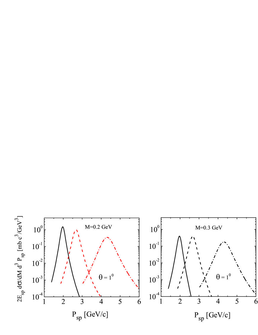
Figure 13: Dependence of the differential cross section $2E_{\rm sp}\displaystyle\frac{d\sigma}{dMd^{3}p_{\rm sp}}$ for the reaction $Dp\to p_{\rm sp}\ np\ e^{+}e^{-}$ on the spectator momentum at two values of the invariant mass of the lepton pair, $M=0.2\ GeV$ (left panel) and $M=0.3\ GeV$ (right panel). The solid, dashed and dot-dashed lines correspond to beam energies $T_{\rm kin}=1.25\ AGeV$, $T_{\rm kin}=1.90\ AGeV$ and $T_{\rm kin}=3.50\ AGeV$ respectively. The spectator is assumed to be detected at $\theta=1^{\circ}$ in the laboratory frame.

In Fig. 13 the dependence of the cross section on the spectator momentum is exhibited for two fixed values of the invariant mass and for $\theta=1^{\circ}$. The three curves (solid, dashed and dot-dashed) in each panel correspond to three different beam energies. It is seen that at each energy the cross section has a maximum at the spectator momentum $\left|{\bf p}_{\rm sp}\right|=\displaystyle\frac{1}{2}\left|{\bf P}_{D}\right|$ (in the anti-laboratory system this corresponds to $\left|{\bf p}_{\rm sp}\right|=0$). The widths of the distributions increase with increasing energy, which is merely an effect of the larger phase space volume.

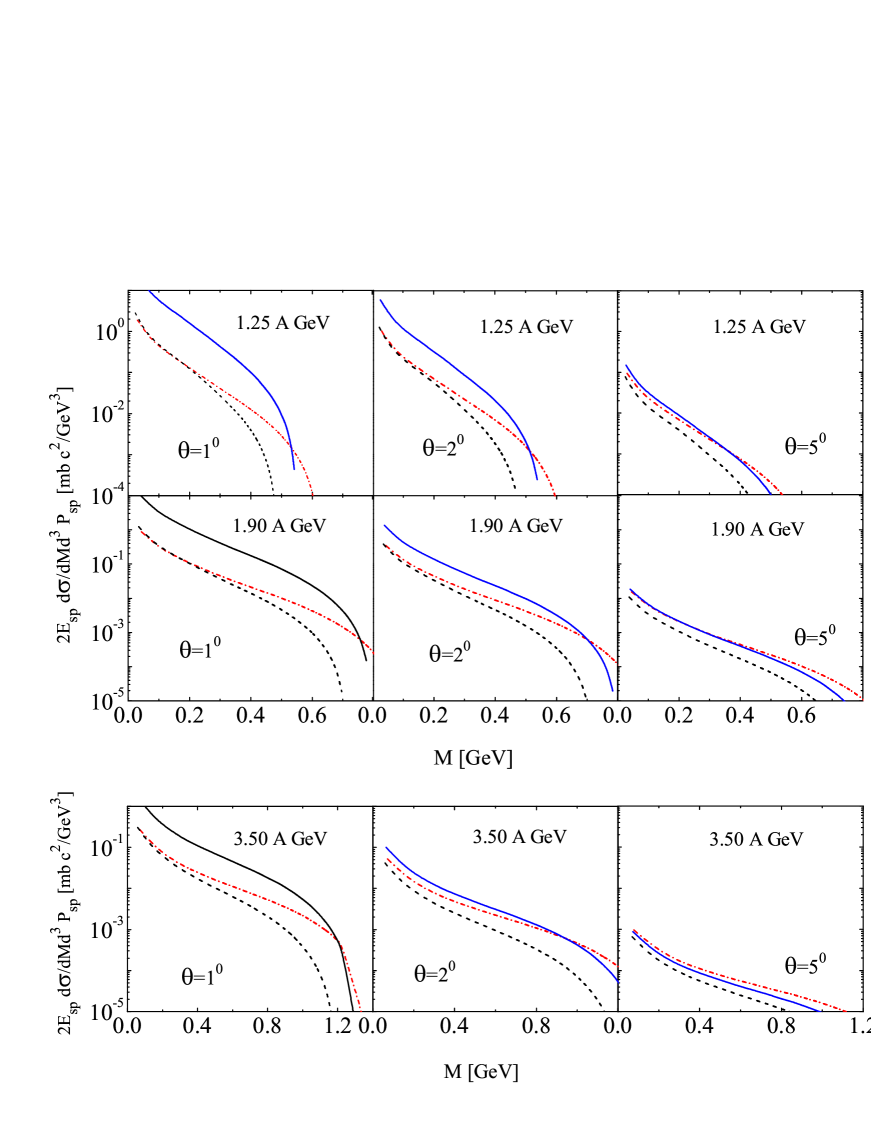
Figure 14: Invariant mass distribution $2E_{\rm sp}\displaystyle\frac{d\sigma}{dMd^{3}p_{\rm sp}}$ for the reaction $Dp\to p_{\rm sp}\ np\ e^{+}e^{-}$ for three values of the deuteron beam energy, $T_{kin}=1.25\ A\>GeV$ (upper panel), $T_{kin}=1.90\ AGeV$ (middle panel) and $T_{kin}=3.5\ A\>GeV$ (lower panel) and three values of the spectator angle in the laboratory system, $\theta=1^{\circ}$ (left column), $\theta=2^{\circ}$(middle column) and $\theta=5^{\circ}$ (right column). Dot-dashed, solid and dashed curves correspond to values of the spectator momentum $\left|{\bf p}_{\rm sp}\right|=0.45\left|{\bf P}_{D}\right|$, $\left|{\bf p}_{\rm sp}\right|=0.50\left|{\bf P}_{D}\right|$ and $\left|{\bf p}_{\rm sp}\right|=0.55\left|{\bf P}_{D}\right|$, respectively.

In Fig. 14 the mass distribution is depicted. The three columns (left, middle and right) correspond to three different angles ($\theta=1^{\circ},\>2^{\circ}$ and $5^{\circ}$), while the three rows (upper, middle and lower) specify three kinetic beam energies, $T_{kin}=1.25,\>1.9,$ and $3.5\ A\>GeV$. For such kinematical conditions the invariant cross section has been calculated at three different values of the spectator momentum, $\left|{\bf p}_{\rm sp}\right|=0.45\>\left|{\bf P}_{D}\right|$ (dot-dashed curves), $\left|{\bf p}_{\rm sp}\right|=0.5\>\left|{\bf P}_{D}\right|$ (solid curves), and $\left|{\bf p}_{\rm sp}\right|=0.55\>\left|{\bf P}_{D}\right|$ (dashed curves), around the maxima of the cross section (cf. Fig. 13). The results in Figs. 13 and 14 do not yet include VMD effects in the $NN$ subprocess, i.e., the results can be considered as estimates of the background contribution.

Fig. 14 illustrates that the shape of the cross section as a function of the invariant mass basically reproduces the one in the $pn$ subprocess. It also seen that at fixed energy and angle the effect of variation of the spectator momentum (dot-dashed, solid and dashed lines in each panel), apart from decreasing the subprocess’s phase space volume with increasing momentum, reduces to a factor being proportional to the deuteron momentum distribution $n_{D}\left(|{\bf p}_{\rm sp}|\right)$ (here ${\bf p}_{\rm sp}$ is the spectator momentum in the anti-laboratory system), as seen from Eq. (53). At moderate values of the invariant mass, e.g., not too close to the kinematical limit, the most favorable conditions for di-electron detection are low angles $\theta\sim 1-2^{\circ}$ and $\left|{\bf p}_{\rm sp}\right|=\displaystyle\frac{1}{2}\left|{\bf P}_{D}\right|$. With $\theta$ increasing the cross section at lower values of $p_{\rm sp}$ becomes comparable with the cross section at $\left|{\bf p}_{\rm sp}\right|=\displaystyle\frac{1}{2}\left|{\bf P}_{D}\right|$. This can be explained that, in spite of $\left|{\bf p}_{\rm sp}\right|<\displaystyle\frac{1}{2}\left|{\bf P}_{D}\right|$, the deuteron momentum distribution $n_{D}\left(|{\bf p}_{\rm sp}|\right)$ decreases (in anti-laboratory system $|{\bf p}_{\rm sp}|\neq 0$ holds), but the phase space increases faster so that the total cross section becomes even larger than at $\left|{\bf p}_{\rm sp}\right|=\displaystyle\frac{1}{2}\left|{\bf P}_{D}\right|$ (where in the anti-laboratory system $|{\bf p}_{\rm sp}|=0$), as the right column in Fig. 14 clearly exhibits.

Finally, in Fig. 15 we present results with VMD effects implemented at the kinetic energy $T_{kin}=3.5\>A\>GeV$, for which the kinematical range of the invariant mass covers the region of $\rho$ and $\omega$ pole masses. As in the $pn$ subprocess the cross section sharply increases near the vector meson poles. The contribution to the peak comes mainly from the $\omega$ excitation. As can be seen in Figs. 7 and 13 at $T_{kin}=1.9\,A\>GeV$ the kinematical limit of the di-electron invariant mass is located just in the vicinity of the vector meson pole masses. In this region the phase space volume for $NN$ reactions shrinks to zero and all possible effects of VMD are masked. However, in the deuteron case the phase space volume can be enlarged by considering spectator momenta with velocities smaller than the initial one. This implies that in the subsystem of the two active nucleons the total energy is larger than in the free $NN$ kinematics. Consequently, effects of sub-threshold vector meson production can be observed in this region. The lower the spectator momentum the larger kinematical range of the allowed di-electron invariant mass can be achieved. However, since the deuteron internal momentum distribution sharply decreases with increasing spectator momentum, the subthreshold di-electron production at very small $\left|{\bf p}_{\rm sp}\right|<\frac{1}{2}\left|{\bf P}_{D}\right|$ (in anti-laboratory the spectator is backward with increasing $|{\bf p}_{\rm sp}|$) is prohibited. Therefore, it is clear that at threshold-near energies there should be a restricted interval for the spectator momentum within which an experimental investigation of the subthreshold production of vector mesons can be achieved. At too large spectator momenta ($\left|{\bf p}_{\rm sp}\right|\gtrsim\displaystyle\frac{1}{2}\left|{\bf P}_{D}\right|$) the suppression originates from the shrinking phase space, whereas too small momenta are restricted by the deuteron’s internal momentum distribution.

In Fig. 16 we present our results for the cross section (53) at the near-threshold energy $T_{kin}=1.9\ A\>GeV$ at two values of the spectator momentum detected in the very forward direction, $\theta=1^{\circ}$. For such a forward kinematics it is quite easy to estimate the effects of enlarging the phase space for the elementary subsystem. At $T_{kin}=1.9\>A\>GeV$ the deuteron momentum is $\left|{\bf P}_{D}\right|=5.36\>GeV/c$ so that, e.g., for the spectator momentum $\left|{\bf p}_{\rm sp}\right|=0.25\>\left|{\bf P}_{D}\right|$, the momentum of the active neutron before interaction is $|{\bf p}_{n}|\simeq 0.75\>\left|{\bf P}_{D}\right|\simeq 4.02\>GeV/c$. This corresponds to a kinetic energy of $T_{kin}\simeq 3.2\>GeV$ in the $np$ subsystem above the vector meson production threshold, hence the cross section at low values of the spectator momenta can leak away into the kinematically forbidden region for the free $np$ process, as seen in Fig. 16. The solid lines correspond to the spectator momenta $\left|{\bf p}_{\rm sp}\right|=0.25\>\left|{\bf P}_{D}\right|$ (left panel) and $\left|{\bf p}_{\rm sp}\right|=0.35\>\left|{\bf P}_{D}\right|$ (right panel) respectively. One observes that as far as the invariant mass is not too close to the threshold, the cross section for the quasi-free kinematics is much larger than at $\left|{\bf p}_{\rm sp}\right|\neq\displaystyle\frac{1}{2}\>\left|{\bf P}_{D}\right|$, i.e., the suppression caused by the deuteron momentum distribution is more important than the effect of enlarging the phase space. In the region close to threshold the quasi-free cross section falls rapidly to zero and the subthreshold cross section becomes predominant. It is also seen that the contribution of $\rho$ and $\omega$ production (dotted lines) is by one order of magnitude above the background. In this case the contribution from the background (the first terms in Eqs. (41) and (42)) can be safely neglected, hence a direct investigation of the vector meson production becomes feasible.

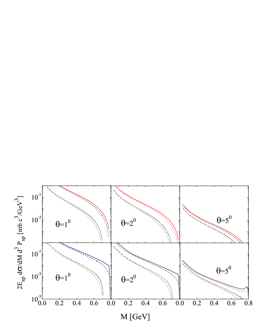
Figure 17: Illustration of FSI effects for the reaction $Dp\to p_{\rm sp}\ pn\ e^{+}e^{-}$ at $T_{kin}=\>1.9\>A\ GeV$ and two values of the spectator momentum. Solid (dashed) lines correspond to results with (without) FSI taken into account for the spectator momentum $\left|{\bf p}_{\rm sp}\right|=0.5\>\left|{\bf P}_{D}\right|$, while the dot-dashed (dotted) lines correspond to $\left|{\bf p}_{\rm sp}\right|=0.55\>\left|{\bf P}_{D}\right|$, respectively. Calculations have been performed at three different values of the spectator angle, $\theta=1^{\circ}$, $2^{\circ}$ and $5^{\circ}$. In the upper row solely contribution from background is displayed, while in the lower row VMD effects have been included as well.

We also have investigated effects of FSI in the reaction $Dp\to p_{\rm sp}pn\>e^{+}e^{-}$. As we mainly consider the parallel kinematics, FSI of the spectator proton with the active $np$ pair can be safely neglected and FSI can be important only in the active $np$ pair. In complete agreement with the factorization formula and previous estimates ourOmega ; titov the effects of FSI are small at small values of the di-electron mass but become visible and important at the kinematical limit. This is illustrated in Fig. 17, where calculations are presented for $T_{kin}=\>1.9\>A\>GeV$ for two values of the spectator momenta. The solid and dashed lines depict results for the spectator momentum $\left|{\bf p}_{\rm sp}\right|=\frac{1}{2}\>\left|{\bf P}_{D}\right|$, while the dot-dashed and dotted lines are for $\left|{\bf p}_{\rm sp}\right|=0.55\>\left|{\bf P}_{D}\right|$. The former value of $\left|{\bf p}_{\rm sp}\right|$ corresponds to the quasi free kinematics, i.e., to the energy of the active $np$ pair near the vector meson production threshold. The latter one determines subthreshold energies even for the $np$ subsystem. Thus, for both values of the spectator momenta the vector meson production threshold is hardly reached and, consequently, FSI effects here are maximized. At lower values of the spectator momentum, as well as at lower di-electron invariant mass, the FSI effects are negligibly small.

IV Summary

In summary we have analyzed different aspects of the di-electron production from the bremsstrahlung mechanism at energies envisaged at HADES HADES for the exclusive reactions $NN\to NN\>e^{+}e^{-}$ and $Dp\to p_{\rm sp}pn\>e^{+}e^{-}$. To calculate the corresponding cross sections we employed an effective meson-nucleon theory with parameters adjusted to elastic $NN$ and inelastic $NN\to NN\pi$ mosel_calc reaction data with $\Delta$ isobars included and with account of vector meson dominance effects. The performed evaluations of bremsstrahlung diagrams can be considered as an estimate of the background contribution, a detailed knowledge of which is a necessary prerequisite for understanding di-electron production in heavy-ion collisions. Our approach is based on covariant evaluations of the corresponding tree level Feynman diagrams with implementing phenomenological form factors and vector meson dominance effects, with particular attention paid on preserving the gauge invariance. The covariance of the approach is achieved by direct relativistic calculations of Feynman diagrams for $NN$ collisions and by implementation of the Bethe-Salpeter formalism for the $Dp$ reaction. The latter case bases on our previously obtained solution of the homogenous Bethe-Salpeter equation with realistic interaction solution .

In accordance with previous results mosel_calc our calculations demonstrate that in the region of invariant masses far from the vector meson production threshold the main contribution to the cross section, in both reactions $pp$ and $pn$, comes from virtual excitations of $\Delta$ isobars. Due to isospin effects the cross section for the reaction $pn\to pn\>e^{+}e^{-}$ is larger than the cross section for $pp\to pp\ e^{+}e^{-}$ by a factor $1.5-3$. Note that because of (i) contributions of the isoscalar $\sigma$ and $\omega$ exchange mesons, (ii) differences in the electromagnetic coupling in $\gamma p$ and $\gamma n$ systems, and (iii) interference effects, the isospin enhancement is not $\sim 9$, as one could naively expect from isospin symmetry considerations. In both reactions, $pn\to pn\>e^{+}e^{-}$ and $pp\to pp\ e^{+}e^{-}$, the bremsstrahlung cross section exhibits a smooth behavior as a function of the di-electron mass. Hence, the bremsstrahlung cross section can be considered as background contribution. In the kinematical range close to the vector meson pole masses the cross section has sharp maxima, clearly indicating that the di-electron production can be also considered as a tool of testing the validity of vector meson dominance. The performed investigations of the vector meson dominance effects show that they contribute in the whole kinematical range. Near the pole masses our diagrammatical approach provides a form for the cross section resembling a two-step model formulae, however it preserves the possibility to trace back the essential differences between the two models (see also discussion in knoll ).

Having computed the diagrams for the process $pn\to pn\>e^{+}e^{-}$ we implemented them for the first time in the reaction $Dp\to p_{\rm sp}\>pn\>e^{+}e^{-}$ with detection of a spectator in the forward direction. The cross section for this process has been evaluated in a covariant approach based on the Bethe-Salpeter formalism. Relativistic effects are negligible here. The Bethe-Salpeter formalism has been used rather for the sake of consistency with the covariant diagrammatical approach and for convenience in using the results from calculations of the subprocess $pn\to pn\>e^{+}e^{-}$. Within the Bethe-Salpeter formalism we derive a factorization formula, i.e., the cross section is cast in a form of a product of two factors, the one entirely originating from the deuteron structure and kinematics, the other one being exactly the cross section of the subprocess $pn\to pn\>e^{+}e^{-}$. In accordance with the factorization formula the shape of the cross section reflects the one in the elementary reaction, except for some corrections from the deuteron wave function. Apart from these common features, an essential difference of the reactions $Dp\to p_{\rm sp}\>pn\>e^{+}e^{-}$ and $np\to\>pn\>e^{+}e^{-}$ can appear. Namely due Fermi motion of nucleons in the deuteron it is possible to find such kinematical conditions within those the energy balance is shifted in favor of the elementary subsystem $np$, so that subthreshold vector meson production becomes feasible. However, the performed analysis shows that the subthreshold cross section is quite low due to a strong suppression originating from the deuteron wave function.

Finally, we found that the effects of final state interaction can be neglected at low values of the di-electron mass. With increasing di-electron mass the final state interaction effects become more important, in particular at the kinematical limit.

Our results are presented for kinematical conditions accessible in forthcoming experiments at HADES HADES ; holzman . Apart from obtaining valuable information for further understanding of di-electron emission in heavy-ion collisions, this also offers a tool for investigation of the interplay of bremsstrahlung process and vector meson dominance effects, i.e., the electromagnetic form factors of nucleons in the time like region not accessible in experiments with on-mass shell particles and the properties of the half-off mass shell nucleon-nucleon amplitude.

V Acknowledgements

Fruitful discussions with H.W. Barz, C. Fuchs, R. Holzmann, J. Knoll and A.I. Titov are gratefully appreciated. L.P.K. would like to thank for the warm hospitality in the Research Center Rossendorf. This work has been supported by BMBF grant 06DR121, GSI-FE and the Heisenberg-Landau program.

Appendix A Isospin in the Rarita-Schwinger formalism

In full analogy with the spin-$3/2$ space, the wave function for an isospin $3/2$-particle, e.g., the $\Delta$, can be written as

$$\chi_{\frac{3}{2}\tau_{\Delta}}=\sum\limits\left\langle 1\lambda\,\frac{1}{2}\tau_{N}\,|\frac{3}{2}\tau_{\Delta}\right\rangle{\bf e}^{*}_{\lambda}\chi_{\frac{1}{2}\tau_{N}},$$ (54)

where $\chi_{\frac{3}{2}}=col\left(\Delta^{++},\Delta^{+},\Delta^{0},\Delta^{-}\right)$, $\chi_{\frac{1}{2}\tau_{N}}$ is the wave function for isospin-$1/2$, and the isospin-$1$ wave function ${\bf e}_{\lambda}\ (\lambda=\pm 1,0)$ has the same structure as in Eq. (99) (see Appendix C).

The definition of the transition matrix $\bf T$ in Eqs. (28) and (29) reads

$$\left\langle\frac{3}{2}\tau_{\Delta}\ |{\bf T}_{\alpha}|\frac{1}{2}\tau_{N}\right\rangle=\left\langle 1\lambda\,\frac{1}{2}\tau_{N}\,|\frac{3}{2}\tau_{\Delta}\right\rangle\left({\bf e}^{*}_{\lambda}\right)_{\alpha}.$$ (55)

Using the completeness of Clebsch-Gordan coefficients one finds

$${\bf T}^{+}_{\alpha}{\bf T}_{\beta}=\delta_{\alpha\beta}-\frac{1}{3}{\mathchar 28956\relax}_{\alpha}{\mathchar 28956\relax}_{\beta}.$$ (56)

The needed Pauli matrices for isospin 1 are

$$\begin{array}[]{ccc}T_{x}=\displaystyle\frac{1}{\sqrt{6}}\left(\begin{array}[]{lr}-\sqrt{3}&0\\ 0&-1\\ 1&0\\ 0&\sqrt{3}\\ \end{array}\right),&T_{y}=\displaystyle\frac{i}{\sqrt{6}}\left(\begin{array}[]{lr}\sqrt{3}&0\\ 0&1\\ 1&0\\ 0&\sqrt{3}\\ \end{array}\right),&T_{z}=\displaystyle\sqrt{\frac{2}{3}}\left(\begin{array}[]{lr}0&0\\ 1&0\\ 0&1\\ 0&0\\ \end{array}\right).\end{array}$$ (70)

Finally, define charge rising (lowering) operators $T_{\pm 1}=(T_{x}\pm iT_{y})/2$ with the following properties

$$\begin{array}[]{lcl}T_{+1}\>|p\rangle\sim|\Delta^{++}\rangle,&\phantom{12}&T_{+1}\>|n\rangle\sim|\Delta^{+}\rangle,\\ T_{-1}\>|p\rangle\sim|\Delta^{0}\rangle,&&T_{-1}\>|n\rangle\sim|\Delta^{-}\rangle\end{array}$$ (73)

to find

$$\begin{array}[]{lcrrrcrr}T_{+1}^{+}T_{z}&=&\frac{1}{3}\tau_{+},&&\phantom{12}&T_{-1}^{+}T_{z}&=&-\frac{1}{3}\tau_{-},\\ T_{z}^{+}T_{+1}&=&-\frac{1}{3}\tau_{+},&&&T_{z}^{+}T_{-1}&=&\frac{1}{3}\tau_{-}.\end{array}$$ (76)

Note that $\left({\bf T}{\mathchar 28956\relax}\right)=2\left(T_{+1}\tau_{-}+T_{-1}\tau_{+}\right)+T_{z}\tau_{z}$ and

$$\begin{array}[]{ccc}T_{z}^{+}T_{z}=\displaystyle\frac{2}{3}\left(\begin{array}[]{cc}\ 1&\ 0\\ \ 0&\ 1\end{array}\right),&\tau_{+}=\left(\begin{array}[]{cc}\ 0&\ 1\\ \ 0&\ 0\end{array}\right)&\tau_{-}=\left(\begin{array}[]{cc}\ 0&\ 0\\ \ 1&\ 0\end{array}\right)\end{array}.$$ (84)

From these equations one finds that the isospin factor for diagonal (with charge conservation) or non-diagonal (with rising or lowering of the charge) terms is $\pm\displaystyle\frac{2}{3}$. Usually pascScholten , in order to simplify the notation, one changes the normalization (56) to

$${\bf T}^{+}_{\alpha}{\bf T}_{\beta}=\delta_{\alpha\beta}-\frac{1}{4}\left[{\mathchar 28956\relax}_{\alpha},{\mathchar 28956\relax}_{\beta}\right].$$ (85)

In this case the factor $\sqrt{\frac{2}{3}}$ is included into the coupling constants. In our calculations we use the normalization (85).

Appendix B Two-step model

In this appendix we establish a correspondence of our diagrammatical approach to models based on a two-step mechanism according to which the cross section for di-electron production is expressed as a product of two terms: (i) production of an on-mass shell vector meson with the mass around its pole value and known width, and (ii) the subsequent decay via the electromagnetic channel conform known branching ratios. To this end we recalculate the cross section Eq. (12) within the VMD conjecture and cast it in a form close to a two-step model. For definiteness, let us calculate the diagram a) in Fig. 2, where now the photon couples the nucleon via an isoscalar vector meson, e.g., the $\omega$ meson. The corresponding part of the amplitude $T$ reads

$$T(q^{2}) = \bar{u}({\bf p}_{1}^{\prime},s_{1}^{\prime})\hat{O}_{mes}(k,P_{2},s_{2},P_{2}^{\prime},s_{2}^{\prime})S(P_{1}-q)\Gamma^{\mu(\omega)}u({\bf p}_{1},s_{1})$$ (86)

$$\times \displaystyle\frac{-g_{\mu\mu^{\prime}}+\displaystyle\frac{q_{\mu}q_{\mu^{\prime}}}{q^{2}}}{q^{2}-M_{0}^{2}}\left(\frac{M_{0}^{2}}{f_{\omega\gamma}}\right)\frac{e^{2}g_{\mu^{\prime}\mu^{\prime\prime}}}{q^{2}}\bar{u}(k_{1},\tilde{s}_{1})\gamma^{\mu^{\prime\prime}}v(k_{2},\tilde{s}_{2}),$$

where formally the operator $\hat{O}_{mes}(k,P_{2},s_{2},P_{2}^{\prime},s_{2}^{\prime})$ includes all the exchange mesons, meson propagators and contributions from the lower vertex Fig. 2a. For further convenience, in the vector propagator in Eq. (86) we replace the quantity $\displaystyle\frac{q_{\mu}q_{\mu}^{\prime}}{M_{0}^{2}}$ by $\displaystyle\frac{q_{\mu}q_{\mu}^{\prime}}{q^{2}}$ (since due to gauge invariance these terms do not contribute to the amplitude (86)). Note that Eq. (86) is valid at any value of $q^{2}$, which generally, could be quite far from the pole mass $M_{0}^{2}$. Let us introduce a hypothetical on-mass shell particle with the invariant mass $s_{V}=s_{\gamma}=q^{2}$ and with quantum numbers as those of $\omega$. Then, for such a particle one can use the completeness relation for its polarization vectors $\xi_{\lambda}(q^{2})$ ($\lambda=0,\pm 1$) to write

$$\sum\limits_{\lambda}\>\xi_{\lambda}^{\mu}(q^{2})\>\xi^{+\mu^{\prime}}_{\lambda}(q^{2})=-g^{\mu\mu^{\prime}}+\displaystyle\frac{q^{\mu}q^{\mu^{\prime}}}{q^{2}}$$ (87)

and

$$\!\!\!\!\!\!\!\!\!\!\!\!T(q^{2}) = \sum\limits_{\lambda}\left[\bar{u}({\bf p}_{1}^{\prime},s_{1}^{\prime})\hat{O}_{mes}(k,P_{2},s_{2},P_{2}^{\prime},s_{2}^{\prime})S(P_{1}-q)\left(\Gamma^{(\omega)}\cdot\xi_{\lambda}^{+}\right)u({\bf p}_{1},s_{1})\right]$$ (88)

$$\times \displaystyle\frac{1}{q^{2}-M_{0}^{2}}\left(\frac{M_{0}^{2}}{f_{\omega\gamma}}\right)\frac{e^{2}}{q^{2}}\bar{u}(k_{1},s_{1})\left(\xi_{\lambda}\cdot\gamma\right)v(k_{2},s_{2})$$

$$\equiv \sum\limits_{\lambda}{\cal A}_{NN\to NNV}\left(q^{2}\neq M_{0}^{2},\lambda\right)\displaystyle\frac{1}{q^{2}-M_{0}^{2}}\left(\frac{M_{0}^{2}}{f_{\omega\gamma}}\right)\frac{e^{2}}{q^{2}}\bar{u}(k_{1},s_{1})\left(\xi_{\lambda}\cdot\gamma\right)v(k_{2},s_{2}),$$

where ${\cal A}_{NN\to NNV}\left(q^{2}\neq M_{0}^{2},\lambda\right)$ corresponds to the production amplitude of a vector particle with invariant mass $q^{2}$ and polarization $\lambda$. The obtained formula has almost the desired factorized form, however, due the dependence upon $\lambda$ of both terms in (88), the factorization is not yet complete. The exact factorization can be accomplished for the squared amplitude after summation over spins and integrating over the leptonic phase space,

$$\frac{1}{4}\sum_{spins}\>\int\left|T(q^{2})\>\right|^{2}R_{2}(q\to k_{1}+k_{2})=$$

$$\frac{1}{4}\sum_{spins}\sum_{\lambda\lambda^{\prime}}\bar{u}({\bf p}_{1}^{\prime},s_{1}^{\prime})\hat{O}_{mes}(k,P_{2},s_{2},P_{2}^{\prime},s_{2}^{\prime})S(P_{1}-q)\left(\Gamma^{(\omega)}\cdot\xi_{\lambda}\right)u({\bf p}_{1},s_{1})\>$$

$$\times\bar{u}({\bf p}_{1},s_{1})\left(\Gamma^{(\omega)}\cdot\xi_{\lambda^{\prime}}^{+}\right)S(P_{1}-q)\hat{O}_{mes}^{+}(k,P_{2},s_{2},P_{2}^{\prime},s_{2}^{\prime})u({\bf p}_{1}^{\prime},s_{1}^{\prime})$$

$$\times\left|\frac{1}{\left(q^{2}-M_{0}^{2}\right)}\right|^{2}\frac{e^{4}}{q^{4}}\int R_{2}(q\to k_{1}+k_{2})\left(\frac{M_{0}^{2}}{f_{\omega\gamma}}\right)^{2}\xi_{\lambda}^{\mu}\>l_{\mu\nu}(k_{1},k_{2})\>\xi_{\lambda^{\prime}}^{+\nu}.$$ (89)

Carrying out the integration over $R_{2}(q\to k_{1}+k_{2})$ and observing that it provides a $\delta_{\lambda\lambda^{\prime}}$ function one gets

$$\frac{1}{4}\sum_{spins}\>\int\left|T(q^{2})\>\right|^{2}R_{2}(q\to k_{1}+k_{2})=$$

$$\ \frac{1}{4}\sum_{spins}\sum_{\lambda}\left|{\cal A}_{NN\to NNV}\left(q^{2}\neq M_{0}^{2},\lambda\right)\right|^{2}\frac{8\pi^{2}\sqrt{s_{\gamma}}\>\Gamma_{em}(q^{2})}{(q^{2}-M_{0}^{2})^{2}+M_{0}^{2}\Gamma_{tot}^{2}(q^{2})},$$ (90)

where the quantity

$$\Gamma_{em}(q^{2})=\frac{4\pi\alpha_{em}^{2}}{3s_{\gamma}\sqrt{s_{\gamma}}}\left(\frac{M_{0}^{2}}{f_{\omega\gamma}}\right)^{2}$$ (91)

plays the role of the electromagnetic decay width of a vector particle into a di-electron via intermediate creation of a virtual photon. Then the cross section can be written in the form

$$\frac{d\sigma}{ds_{\gamma}} = \left[\frac{1}{2(2\pi)^{5}\sqrt{\lambda(s,m^{2},m^{2})}}\frac{1}{4}\sum_{spins}\int ds_{12}R_{2}(P_{1}+P_{2}\to P_{V}+P_{12})R_{2}(P_{12}\to P_{1}^{\prime}+P_{2}^{\prime})\right.$$ (92)

$$\times \left.\left|{\cal A}_{NN\to NNV}\left(q^{2}\neq M_{0}^{2},\lambda\right)\phantom{\frac{1^{2}}{2^{2}}}\right|^{2}\right]\frac{\sqrt{s_{\gamma}}\>\Gamma_{em}(q^{2})/\pi}{(q^{2}-M_{0}^{2})^{2}+M_{0}^{2}\Gamma_{tot}^{2}(q^{2})},$$

where the expression in square brackets can be interpreted as cross section for the creation of a vector particle with the mass $s_{\gamma}=q^{2}$ in a $NN$ process,

$$\frac{d\sigma}{ds_{\gamma}}=\sigma_{V}(q^{2}\neq M_{0}^{2})\>\frac{\sqrt{s_{\gamma}}\>\Gamma_{em}(q^{2})/\pi}{(q^{2}-M_{0}^{2})^{2}+M_{0}^{2}\Gamma_{tot}^{2}(q^{2})}.$$ (93)

It is worth emphasizing that the invariant mass $q^{2}$ varies in the whole kinematical range, $0<\>q^{2}\><\>q^{2}_{max}$. Hence, the form of the cross section (93) is valid at any initial energy, including deep-subthreshold values, $q^{2}_{max}\ll M_{0}^{2}$. Therefore, at such invariant masses the cross section can be considered as background contribution to di-electron production. In the very vicinity of the pole masses, $q^{2}\to M_{0}^{2}$, the cross section (93) becomes

$$\frac{d\sigma}{ds_{\gamma}}=\sigma_{\omega}(M_{0}^{2})\>\frac{\Gamma_{em}/\left(4\pi\sqrt{s_{\gamma}}\right)}{\left(\sqrt{s_{\gamma}}-M_{0}\right)^{2}+\Gamma_{tot}^{2}/4}$$ (94)

which exactly coincides with results of the two-step model. Remind that our diagrammatical approach can be related to the two-step model only if (i) one considers the cross section integrated over the di-electron phase space, (ii) the invariant mass $s_{\gamma}$ is not too far from the pole masses, (iii) interferences between different kinds of vector mesons, $\omega$ and $\rho$, are disregarded, and (iv) the contributions of other diagrams (e.g., with $\Delta$ isobars) are neglected.

Appendix C Factorization

The BS amplitudes in the deuteron rest system are of the form quad ; Tjon

$$\Psi_{{\cal M}_{D}}^{S^{++}}(P_{n},p_{\rm sp}) = {\cal N}(\hat{k}_{n}+m)\frac{1+\gamma_{0}}{2}\hat{\xi}_{{\cal M}_{M}}(\hat{p}_{\rm sp}-m)\phi_{S}(p_{0},|{\bf P}_{n}|),$$ (95)

$$\Psi_{{\cal M}_{D}}^{D^{++}}(P_{n},p_{\rm sp}) = -\frac{{\cal N}}{\sqrt{2}}(\hat{k}_{n}+m)\frac{1+\gamma_{0}}{2}\left(\hat{\xi}_{{\cal M}_{D}}+\frac{3}{2|{\bf P}_{n}|^{2}}(\hat{k}_{n}-\hat{p}_{\rm sp})(p\xi_{M})\right)$$

$$\times(\hat{p}_{\rm sp}-m)\phi_{D}(p_{0},|{\bf P}_{n}|),$$

where $k_{n}$ is an on-mass shell four vector related to the off-mass shell neutron vector $P_{n}$ as follows (in anti-laboratory system one has ${\bf P}_{n}=-{\bf p}_{\rm sp}$)

$$k_{n}=(E_{{\bf k}_{n}},{\bf P}_{n}),\quad E_{{\bf k}_{n}}=\sqrt{{\bf P}_{n}^{2}+m^{2}};\quad p=(p_{0},{\bf P}_{n}),\quad p_{0}=\frac{1}{2}M_{D}-E_{\rm sp}.$$ (96)

$\phi_{S,D}(p_{0},|{\bf P}_{n}|)$ are the partial scalar amplitudes related to the corresponding partial vertices as

$$\phi_{S,D}(p_{0},|{\bf P}_{n}|)=\displaystyle\frac{G_{S,D}(p_{0},|{\bf P}_{n}|)}{\left(\displaystyle\frac{M_{D}}{2}-E_{\rm sp}\right)^{2}-p_{0}^{2}}.$$ (97)

In Eq. (95) $M_{D}$ is the deuteron mass,and the normalization factor is ${\cal N}=\displaystyle\frac{1}{\sqrt{8\pi}}\displaystyle\frac{1}{2E_{\rm sp}(E_{\rm sp}+m)}$.

The components of the polarization vector of a vector particle moving with 4-momentum $p=(E,{\bf p})$ having the polarization projection ${\cal M}=\pm 1,\,0$ and mass $M$ are

$$\xi_{\cal M}=\left(\frac{\bf p{\mathchar 28952\relax}_{\cal M}}{M},{\mathchar 28952\relax}_{\cal M}+{\bf p}\frac{\bf p{\mathchar 28952\relax}_{\cal M}}{M(E_{\bf p}+M)}\right),$$ (98)

where ${\mathchar 28952\relax}_{\cal M}$ is the polarization vector for the particle at rest with

$$\begin{array}[]{ccc}{\mathchar 28952\relax}_{+1}=-\displaystyle\frac{1}{\sqrt{2}}\,\left(\begin{array}[]{c}1\\ i\\ 0\end{array}\right),&\quad{\mathchar 28952\relax}_{-1}=\displaystyle\frac{1}{\sqrt{2}}\left(\begin{array}[]{c}1\\ -i\\ 0\end{array}\right),&\quad{\mathchar 28952\relax}_{0}=\left(\begin{array}[]{c}0\\ 0\\ 1\end{array}\right).\end{array}$$ (99)

The Dirac spinors, normalized as $\bar{u}(p)u(p)=2m$ and $\bar{v}(p)v(p)=-2m$, read

$$u({\bf p},s)=\sqrt{m+E_{{\bf p}}}\left(\begin{array}[]{c}\chi_{s}\\ \displaystyle\frac{{\mathchar 28955\relax}{\bf p}}{m+E_{{\bf p}}}\chi_{s}\end{array}\right),\quad\quad v({\bf p}\,,s)=\sqrt{m+E_{{\bf p}}}\left(\begin{array}[]{c}\displaystyle\frac{{\mathchar 28955\relax}{\bf p}}{m+E_{{\bf p}}}\widetilde{\chi}_{s}\\ \widetilde{\chi}_{s}\end{array}\right),$$ (104)

where $\widetilde{\chi}_{s}\equiv-i\sigma_{y}\chi_{s}$, and $\chi_{s}$ denotes the usual two-dimensional Pauli spinor. Note that the denominator in (97) is zero when one particle (the spectator in our case) is on-mass shell. This singularity is apparent since it is exactly compensated by the factors $(\hat{p}_{\rm sp}-m)\ \tilde{S}^{-1}(p_{\rm sp})=p_{\rm sp}^{2}-m^{2}=0$ from (95) and (47). In terms of the main BS components the ”deuteron spinor” ${\cal V}_{D}$ (48) can be written in as

$${\cal V}_{D}={\cal N}(p_{\rm sp}^{2}-m^{2})\ \left(\phi_{S}V_{S}-\frac{1}{\sqrt{2}}\phi_{D}V_{S}-\frac{1}{\sqrt{2}}\phi_{D}\ V_{D}\right),$$ (105)

where

$$V_{S} = (\hat{k}_{n}+m)\left(\begin{array}[]{cc}1&0\\ 0&0\end{array}\right)\left(\begin{array}[]{cc}0&-({\mathchar 28955\relax}{\mathchar 28952\relax})\\ ({\mathchar 28955\relax}{\mathchar 28952\relax})&0\end{array}\right)\sqrt{E_{\rm sp}+m}\left(\begin{array}[]{c}-\displaystyle\frac{({\mathchar 28955\relax}{\bf P}_{n})}{E_{\rm sp}+m}\widetilde{\chi}_{s}\\ \widetilde{\chi}_{s}\end{array}\right)$$ (112)

$$= \sqrt{E_{\rm sp}+m}\left(\begin{array}[]{cc}0&-(E_{\rm sp}+m)({\mathchar 28955\relax}{\mathchar 28952\relax})\\ 0&-({\bf P}_{n}{\mathchar 28955\relax})({\mathchar 28955\relax}{\mathchar 28952\relax})\end{array}\right)\left(\begin{array}[]{c}-\displaystyle\frac{({\mathchar 28955\relax}{\bf P}_{n})}{E_{\rm sp}+m}\widetilde{\chi}_{s}\\[5.69054pt] \widetilde{\chi}_{s}\end{array}\right)$$ (117)

$$= -\left({E_{\rm sp}+m}\right)^{3/2}\left(\begin{array}[]{c}({\mathchar 28955\relax}{\mathchar 28952\relax})\widetilde{\chi}_{s}\\[5.69054pt] \displaystyle\frac{({\bf P}_{n}{\mathchar 28955\relax})({\mathchar 28955\relax}{\mathchar 28952\relax})}{E_{\rm sp}+m}\widetilde{\chi}_{s}\end{array}\right),$$ (120)

$$V_{D} = \displaystyle\frac{3({\bf P}_{n}{\mathchar 28952\relax})}{{\bf P}_{n}^{2}}\left(\begin{array}[]{cc}E_{\rm sp}+m&-({\bf P}_{n}{\mathchar 28955\relax})\\ ({\bf P}_{n}{\mathchar 28955\relax})&-E_{\rm sp}+m\end{array}\right)\left(\begin{array}[]{cc}1&0\\ 0&0\end{array}\right)\left(\begin{array}[]{cc}0&({\bf P}_{n}{\mathchar 28955\relax})\\ -({\bf P}_{n}{\mathchar 28955\relax})&0\end{array}\right)$$ (130)

$$\times\sqrt{E_{\rm sp}+m}\left(\begin{array}[]{c}-\displaystyle\frac{({\mathchar 28955\relax}{\bf P}_{n})}{E_{\rm sp}+m}\widetilde{\chi}_{s}\\ \widetilde{\chi}_{s}\end{array}\right)$$

$$= \left(E_{\rm sp}+m\right)^{3/2}\displaystyle\frac{3({\bf P}_{n}{\mathchar 28952\relax})}{{\bf P}_{n}^{2}}\left(\begin{array}[]{c}({\bf P}_{n}{\mathchar 28955\relax})\widetilde{\chi}_{s}\\[5.69054pt] \displaystyle\frac{{\bf P}_{n}^{2}}{E_{\rm sp}+m}\widetilde{\chi}_{s}\end{array}\right).$$ (133)

From (112) and (133) one finds

$$\sum\limits_{{\cal M}_{D},s}V_{S}\bar{V}_{S}=3(E_{\rm sp}+m)^{2}(\hat{k}_{n}+m),$$ (134)

$$\sum\limits_{{\cal M}_{D},s}V_{D}\bar{V}_{D}=9(E_{\rm sp}+m)^{2}(\hat{k}_{n}+m),$$ (135)

$$\sum\limits_{{\cal M}_{D},s}V_{S}\bar{V}_{D}=\sum\limits_{{\cal M}_{D},s}V_{D}\bar{V}_{S}=-3(E_{\rm sp}+m)^{2}(\hat{k}_{n}+m).$$ (136)

Now it is straightforward to obtain (50) from Eqs. (95) - (136). In Eq. (50) the deuteron wave functions $U_{S,D}(|{\bf p}_{\rm sp}|)$ are related with the half off-mass shell vertices $G_{S,D}$ (97) as

$$U_{S,D}(|{\bf p}_{\rm sp}|)=\displaystyle\frac{G_{S,D}(p_{0}=\frac{1}{2}M_{D}-E_{\rm sp},|{\bf p}_{\rm sp}|)}{4\pi\sqrt{2M_{D}}\left(M_{D}-2E_{\rm sp}\right)}.$$ (137)

Meson		$\displaystyle\frac{g^{2}_{NNM}}{4\pi}$	qqq$\kappa$qqq	l		$\Lambda$
				($GeV^{-1}$)		(GeV)
$\pi$		12.562	-	0.1133		1.005
$\sigma$		2.340	-	0.1070		1.952
$\rho$		0.317	6.03	0.1800		1.607
$\omega$		46.035	0	0.0985		0.984

Table 1: OBE parameters used in the calculations (cf. Eq. (17) and Ref. mosel_calc ). Note that $f_{NN\pi}=\displaystyle\frac{\mu_{\pi}}{2m}g_{NN\pi}$.

Figure 4: Invariant mass distribution of a $e^{+}e^{-}$ pair in proton-proton collisions. The dashed (dotted) curves depict the contribution of diagrams with bremsstrahlung from $\gamma\Delta N$ ($\gamma NN$) vertices. The solid lines are the results of calculations of the total cross section as coherent sums of nucleon and $\Delta$ contributions. The calculations have been performed at DLS energies DLS and are directly comparably with results of mosel_calc .

Figure 5: The same as in Fig. 4 but for $pn$ reactions. The dotted curves include also contributions from $\gamma\pi NN$ vertices.

Figure 6: Invariant mass distribution of di-electrons in $pp$ reactions at energies envisaged in experiments at HADES HADES . Notation as in Fig. 4.

Figure 7: The same as in Fig. 6 but for $pn$ reactions.

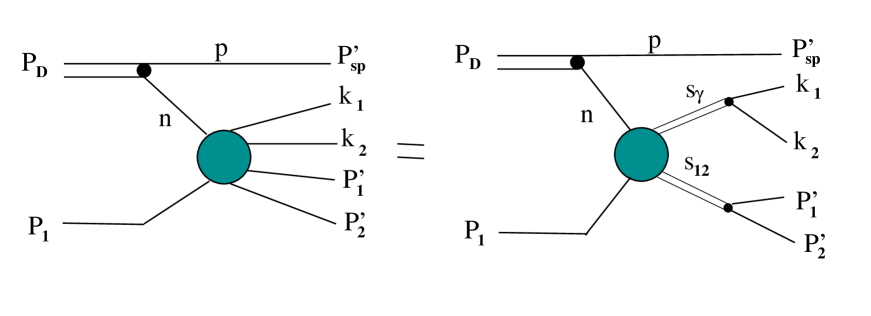
Figure 12: Kinematics of the process $D(P_{D})+p(P_{1})\to p(P_{\rm sp}+p(P_{1}^{\prime})+n(P_{2}^{\prime})+e^{+}(k_{1})+e^{-}(k_{2})$ within the spectator mechanism.

Figure 15: Invariant mass distribution $2E_{\rm sp}\displaystyle\frac{d\sigma}{dMd^{3}p_{\rm sp}}$ for the reaction $Dp\to p_{\rm sp}\ np\ e^{+}e^{-}$, at deuteron beam energy $T_{kin}=3.5\ AGeV$ and three values of the spectator angle in the laboratory system, $\theta=1^{\circ},2^{\circ}$ and $5^{\circ}$. Dot-dashed, solid and dashed curves correspond to values of the spectator momentum $\left|{\bf p}_{\rm sp}\right|=0.45\left|{\bf P}_{D}\right|$, $\left|{\bf p}_{\rm sp}\right|=0.50\left|{\bf P}_{D}\right|$ and $\left|{\bf p}_{\rm sp}\right|=0.55\left|{\bf P}_{D}\right|$, respectively. Effects of VMD have been taken into account.

Figure 16: Effects of sub-threshold vector meson production in the reaction $Dp\to p_{\rm sp}\ pn\ e^{+}e^{-}$ at low values of the spectator momentum, $\left|{\bf p}_{\rm sp}\right|=0.25\>\left|{\bf P}_{D}\right|$ (left panel) and $\left|{\bf p}_{\rm sp}\right|=0.35\>\left|{\bf P}_{D}\right|$ (right panel). Dashed lines depict the background contribution, dotted lines are separate contributions from $\rho$ and $\omega$ mesons, and solid lines are for the total cross section.

References

-
(1)
P. Lichard, Phys. Rev. D 51 (1995) 6017; hep-ph/9812211;
J. Zhang, R. Tabti, C. Gale, K. Haglin, Int. J. Mod. Phys. E6 (1997) 475. - (2) R. Shyam, U. Mosel, Phys. Rev. C 67 (2003) 065202.
-
(3)
C. Gale, J. Kapusta, Phys. Rev. C 35 (1987) 2107; Phys. Rev C 40 (1989) 2397;
K. Haglin, J. Kapusta, C. Gale, Phys. Lett. B 224 (1989) 433;
K. Haglin, Ann. Phys. 212 (1991) 84
L. Xiong, Z.G. Wu, C.M. Ko, J.Q. Wu, Nucl. Phys. A 512 (1990) 772;
L.A. Winkelmann, H. Stöcker, W. Greiner, H. Sorge, Phys. Lett. B 298 (1993) 22;
A.I. Titov, B. Kämpfer, E.L. Bratkovskaya, Phys. Rev. C 51 (1995) 227. - (4) C. Ernst, S.A. Bass, N. Belkacem, H. Stöcker, W. Greiner, Phys. Rev. C 58 (1998) 447.
- (5) K. Tsushima, K. Nakayama, Phys. Rev. C 68 (2003) 034612.
-
(6)
C. Fuchs, A. Faessler, D. Cozma, B.V. Martemyanov, M. Krivoruchenko, Nucl. Phys. A 755 (2005) 499c
A. Faessler, C. Fuchs, M. Krivoruchenko, B.V. Martemyanov, Phys. Rev. C 70 (2004) 035211;
C. Fuchs, M. Krivoruchenko, H.L. Yadav, A. Faessler, B.V. Martemyanov, K. Shekhter, Phys. Rev. C 67 (2003) 025202. - (7) L.P. Kaptari, B, Kämpfer, Eur. Phys. J. A 23 (2005) 291.
-
(8)
M.F.M. Lutz, M. Soyeur, nucl-th/0503087;
M.F.M. Lutz, Gy. Wolf, B. Friman, Nucl. Phys. A 706 (2002) 431. -
(9)
A.Yu. Umnikov, L.P. Kaptari, F.C Khanna, Phys. Rev. C 56 (1997) 1700;
A.Yu. Umnikov, L.P. Kaptari, K.Yu. Kazakov, F.C. Khanna, Phys. Lett. B334 (1994) 163;
A.Yu. Umnikov, Z. Phys. A 357 (1997) 333. - (10) P. Salabura et al. (HADES Collaboration), Acta Phys. Polon. B 35 (2004) 1119.
- (11) R. Holzmann et al. (HADES Collaboration), Prog. Part. Nucl. Phys. 53 (2004) 49.
- (12) L.P. Kaptari, B. Kämpfer, S.S. Semikh. J. Phys. G30 (2004) 1115.
-
(13)
S. Okubo, Phys. Lett. 5 (1963) 165;
G. Zweig, CERN Report 8419/TH 412 (1964);
I. Iizuka, Prog. Theor. Phys. Suppl. 37/38 (1966) 21. - (14) K. Haglin, C. Gale, Phys. Rev. C 49 (1994) 401.
- (15) E.L. Bratkovskaya, W. Cassing, U. Mosel, Nucl. Phys. A 686 (2001) 568.
- (16) L.P. Kaptari, B, Kämpfer, Eur. Phys. J. A 14 (2002) 211.
- (17) R. Shyam, Phys. Rev. C 60 (1999) 055213.
- (18) R. Machleidt, Adv. Nucl. Phys. 19 (1989) 189; Phys. Rev. C 63 (2001) 024001.
- (19) W.S. Chung, G.Q. Li, C.M. Ko, Phys. Lett. B 401 (1997) 1.
- (20) G. Wolf, G. Batko, W. Cassing, U. Mosel, K. Niita, M. Schäfer, Nucl. Phys. A 517 (1990) 615.
-
(21)
J. Ward, Phys. Rev. 78 (1950) 182;
Y. Takahashi, Nuovo Cim. 6 (1957) 371. - (22) H.W.L. Naus, J.H. Koch, Phys. Rev C 36 (1987) 2459.
-
(23)
A. Yu. Korchin, O. Scholten, Nucl. Phys. A 581 (1995) 493);
A. Yu. Korchin, O. Scholten, F. de Jong, Phys. Lett. B 402 (1997) 1. - (24) P.C. Tiemeijer, J.A. Tjon, Phys. Rev. C 42 (1990) 599.
- (25) H.C. Dönges, M. Schäfer, U. Mosel, Phys. Rev. C 51 (1995) 950.
- (26) F. Gross, D.O. Riska, Phys. Rev. C 36 (1987) 1928.
- (27) J.F. Mathiot, Nucl. Phys. A 412 (1984) 201.
- (28) M. Schäfer, H.C. Dönges, A. Engel, U. Mosel, Nucl. Phys. A 575 (1994) 429.
- (29) N.M. Kroll, M.A. Ruderman, Phys. Rev. 93 (1954) 233.
- (30) T. de Forest Jr., Nucl. Phys. A 392 (1983) 232.
- (31) J.J. Sakurai, Currents and Mesons (University of Chicago Press, Chicago, 1969).
- (32) F. de Jong, U. Mosel, Phys. Lett. B 392 (1997) 273.
- (33) G. Höhler, E. Pietarinen, I. Sabba-Stefanescu, Nucl. Phys. B 224 (1976) 505.
- (34) V. Pascalutsa, O. Scholten, Nucl. Phys. A 591 (1995) 658.
- (35) C. Gale, J. Kapusta, Phys. Rev. C 49 (1994) 401.
- (36) K. Holinde, R. Machleidt, M.R. Anastasio, A. Faessler, H. Müther, Phys. Rev. C 18 (1978) 870.
- (37) G.E. Brown, W. Weise, Phys. Rep. 22 (1975) 279.
-
(38)
V. Pascalutsa, Phys. Rev. D 58 (1998) 096002;
V. Pascalutsa, R. Timmermans, Phys. Rev. C 60 (1999) 042201(R). -
(39)
R.M. Davidson, Nimai C. Mukhopadhyay, S. Wittman, Phys. Rev. D 43 (1991) 71;
M. Benmerrouche, R.M. Davidson, Nimai C. Mukhopadhyay, Phys. Rev. C 39 (1989) 2339. - (40) M.G. Olsson. E.T. Osypowski, Nucl. Phys. B 87 (1975)451.
-
(41)
J.W. van Orden, T.W. Donelly, Ann. Phys. 131 (1981) 451;
H. Garcilazo, E.M. de Guerra, Nucl. Phys. A 562 (1993) 521. - (42) V. Shklyar, H. Lenske, U. Mosel, G. Penner, Phys. Rev. C 71 (2005) 055206
-
(43)
S. Weinberg, Phys. Rev. 133 (1964) B1318;
R.E. Behrends, C. Fronsdal, Phys. Rev. 106 (1957) 345;
S.-J. Chang, Phys. Rev. 161 (1967) 161. - (44) M. J. Dekker, P. J. Brussaard, R. J. Van de Graaff, J. A. Tjon, Phys. Rev. C 49 (1994) 2650.
- (45) A.I. Titov, B. Kämpfer, B.L. Reznik, Phys. Rev. C 65 (2002) 065202.
- (46) M. Post, S. Leupold, U. Mosel, Nucl. Phys. A 689 (2001) 753.
- (47) H.T. Williams, Phys. Rev. C 39 (1989) 2339.
- (48) R. Shyam, Phys. Rev. C 60 (1999) 055213.
- (49) T. Feuster, U. Mosel, Nucl. Phys. A 612 (1997) 375.
- (50) G. Caia, V. Pascalutsa, J.A. Tjon, L.E. Wright, Phys. Rev. C 70 (2004) 032201(R).
-
(51)
W. Rarita, J. Schwinger, Phys. Rev. 60 (1941) 61;
A. Aurilia, H. Umezawa, Phys. Rev. 182 (1969) 1682. - (52) W.K. Wilson, S. Beedoe, R. Rossingarn, M. Bougteb et al., Phys. Rev. C 57 (1998) 1865.
- (53) M.F.M. Lutz, B. Friman, M. Soyeur, Nucl. Phys. A 713 (2003) 97.
- (54) S. Dubnicka, Nuovo Cimento A 103 (1990) 1417.
- (55) M. Gari, W. Krümpelmann, Z. Phys. A 322 (1985) 689.
- (56) N.M. Kroll, T.D. Lee, B. Zumino, Phys. Rev. 157 (1967) 1376.
- (57) B. Friman, M. Soyeur, Nucl. Phys. A 600 (1996) 477.
- (58) J. Knoll, Prog. Part. Nucl. Phys 42 (1999) 177.
- (59) A.I. Titov, B. Kämpfer, B.L. Reznik, Eur. Phys. J., A 7 (2000) 543.
- (60) J. Gillespie, ” Final State Interactions”, Holden-Day Advanced Physics Monographs, 1964.
- (61) M.M. Sargsian, T.V. Abrahamyan, M.I. Strikman, L.L. Frankfurt, nucl-th/0406020.
-
(62)
C. Ciofi degli Atti, L.P. Kaptari, Phys. Rev. C 71 (2005) 024005;
M.A. Braun, C. Ciofi degli Atti, L.P. Kaptari, H. Morita, nucl-th/0308069. - (63) L.P. Kaptari, B. Kämpfer, S.M. Dorkin, S.S. Semikh, Phys. Rev. C 57 (1998) 1097; Phys. Lett. B 404 (1997) 8.
-
(64)
L.P. Kaptari, A.Yu. Umnikov, S.G. Bondarenko, K.Yu. Kazakov, F.C. Khanna, B. Kämpfer, Phys. Rev. C 54 (1996) 986;
C. Ciofi degli Atti, D. Faralli, A.Yu. Umnikov, L.P. Kaptari, Phys. Rev. C 60 (1999) 034003. -
(65)
B.D. Keister, J.A. Tjon, Phys. Rev. C 26 (1982) 578;
G. Rupp, J.A. Tjon, Phys. Rev. C 41 (1990) 472;
J.J. Kubis, Phys. Rev. D 6 (1972) 547;
M.J. Zuilhof, J.A. Tjon, Phys. Rev. C 22 (1980) 2369.