Direct Reactions with Exotic Nuclei

Abstract

We discuss recent work on Coulomb dissociation and an effective-range theory of low-lying electromagnetic strength of halo nuclei. We propose to study Coulomb dissociation of a halo nucleus bound by a zero-range potential as a homework problem. We study the transition from stripping to bound and unbound states and point out in this context that the Trojan-Horse method is a suitable tool to investigate subthreshold resonances.

1 Introduction and Overview

With the exotic beam facilities all over the world - and more are to come - direct reaction theories are experiencing a renaissance. We report on recent work - just finished and in progress - on Coulomb dissociation of halo nuclei tybaprl ; tyba04 and on transfer reactions to bound and scattering states. We hope to report on further progress at the next workshop at MSU/ANL/INT/JINA/RIA or elsewhere.

Electromagnetic strength functions of halo nuclei exhibit universal features that can be described in terms of characteristic scale parameters. For a nucleus with nucleon+core structure the reduced transition probability, as determined, e.g., by Coulomb dissociation experiments (for a review see ppnp ; hirsch ), shows a typical shape that depends on the nucleon separation energy and the orbital momenta in the initial and final states. The sensitivity to the final-state interaction (FSI) between the nucleon and the core can be studied systematically by varying the strength of the interaction in the continuum. In the case of neutron+core nuclei analytical results for the reduced transition probabilities are obtained by introducing an effective-range expansion. The scaling with the relevant parameters is found explicitly. General trends are observed by studying several examples of neutron+core and proton+core nuclei in a single-particle model assuming Woods-Saxon potentials. Many important features of the neutron halo case can be obtained already from a square-well model. Rather simple analytical formulae are found. The nucleon-core interaction in the continuum affects the determination of astrophysical S factors at zero energy in the method of asymptotic normalisation coefficients (ANC). It is also relevant for the extrapolation of radiative capture cross sections to low energies.

Coulomb dissociation of a neutron halo nucleus in the limit of a zero-range neutron-core interaction in the Coulomb field of a target nucleus can be studied in various limits of the parameter space and rather simple analytical solutions can be found. We propose to solve the scattering problem for this model Hamiltonian by means of the various advanced numerical methods that are available nowadays. In this way their range of applicability can be studied by comparison to the analytical benchmark solutions.

The Trojan-Horse Method tyba02 ; fus03 is a particular case of transfer reactions to the continuum under quasi-free scattering conditions. Special attention is paid to the transition from reactions to bound and unbound states and the role of subthreshold resonances. Since the binding energies of nuclei close to the drip line tend to be small, this is expected to be an important general feature in exotic nuclei.

2 Effective Range Theory of Halo Nuclei

At low energies the effect of the nuclear potential is conveniently described by the effective-range expansion Bet49 . An effective-range approach for the electromagnetic strength distribution in neutron halo nuclei was introduced in tybaprl and applied to the single neutron halo nucleus ¹¹Be. Recently, the same method was applied to the description of electromagnetic dipole strength in ²³O Noc04 . A systematic study sheds light on the sensitivity of the electromagnetic strength distribution to the interaction in the continuum. We expose the dependence on the binding energy of the nucleon and on the angular momentum quantum numbers. Our approach extends the familiar textbook case of the deuteron, that can be considered as the prime example of a halo nucleus, to arbitrary nucleon+core systems, for related work see kala ; besu ; be . We also investigate in detail the square-well potential model. It has great merits: it can be solved analytically, it shows the main characteristic features and leads to rather simple and transparent formulae. As far as we know, some of these formulae have not been published before. These explicit results can be compared to our general theory for low energies (effective-range approach) and also to more realistic Woods-Saxon models. Due to shape independence, the results of these various approaches will not differ for low energies. It will be interesting to delineate the range of validity of the simple models.

Our effective-range approach is closely related to effective field theories that are nowadays used for the description of the nucleon-nucleon system and halo nuclei Ber02 . The characteristic low-energy parameters are linked to QCD in systematic expansions. Similar methods are also used in the study of exotic atoms ($\pi^{-}A$, $\pi^{+}\pi^{-}$, $\pi^{-}p$, …) in terms of effective-range parameters. The close relation of effective field theory to the effective-range approach for hadronic atoms was discussed in Ref. Hol99 .

In Fig. 1 we show the application of the method to the electromagnetic dipole strength in ¹¹Be. The reduced transition probability was deduced from high-energy ¹¹Be Coulomb dissociation at GSI palit . Using a cutoff radius of $R=2.78$ fm and an inverse bound-state decay length of $q=0.1486$ fm^-1 as input parameters we extract an ANC of $C_{0}=0.724(8)$ fm^-1/2 from the fit to the experimental data. The ANC can be converted to a spectroscopic factor of $C^{2}S=0.704(15)$ that is consistent with results from other methods. In the lowest order of the effective-range expansion the phase shift $\delta_{l}^{j}$ in the partial wave with orbital angular momentum $l$ and total angular momentum $j$ is written as $\tan\delta_{l}^{j}=-(xc_{l}^{j}\gamma)^{2l+1}$, where $\gamma=qR=0.4132<1$ is the halo expansion parameter and $x=k/q=\sqrt{E/S_{n}}$ with the neutron separation energy $S_{n}$. The parameter $c_{l}^{j}$ corresponds to the scattering length $a_{l}^{j}=(c_{l}^{j}R)^{2l+1}$. We obtain $c^{3/2}_{1}=-0.41(86,-20)$ and $c^{1/2}_{1}=2.77(13,-14)$. The latter is unnaturally large because of the existence of a bound $\frac{1}{2}^{-}$ state close to the neutron breakup threshold in ¹¹Be. For a further discussion we refer to tybaprl .

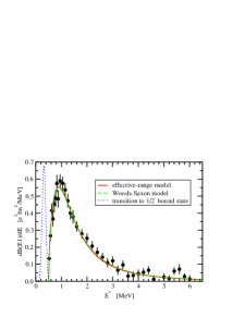
Figure 1: Reduced probability for dipole transitions as a function of the excitation energy $E^{\ast}=E+S_{n}$ in comparison to experimental data extracted from Coulomb dissociation of ¹¹Be palit .

3 Homework problem

We consider a three-body system consisting of a neutron $n$, a core $c$ and an (infinitely heavy) target nucleus with charge $Ze$. The Hamiltonian is given by

$$H=T+V_{cZ}+V_{nc}$$ (1)

where $T$ is the kinetic energy. The Coulomb interaction between the core and the target is given by $V_{cZ}=ZZ_{c}e^{2}/r_{c}$ and $V_{nc}$ is a zero-range interaction between $c$ and $n$. The s-wave bound state of the $a=(c+n)$ system is given by the wave function $\Phi_{0}=\sqrt{q/(2\pi)}\exp{(-qr)}/r$, where $q$ is related to the binding energy $E_{b}$ by $E_{b}=\hbar^{2}q^{2}/(2\mu)$ and the reduced mass of the $c+n$ system is denoted by $\mu$. We refer to ppnp (see especially Ch. 4 there) for details. (The present homework problem is simpler than the one assigned by I. Thompson: in his case there is a p-wave bound state in ⁸Li, and, in addition, the interactions between the target and the projectile are much more complicated.)

One can study elastic scattering (influence of the polarisation potential) as well as breakup of the halo nucleus $a$ in the Coulomb field of the target nucleus $Z$. Although the Coulomb dissociation of this zero-range halo nucleus is governed by a rather simple Hamiltonian, the solution of this problem is nontrivial, as is often the case in physics. This model is also relevant for the Oppenheimer-Phillips process (polarisation of a deuteron in the Coulomb field of a nucleus) opp , see also ben for a criticism. The parameter space is given by the charge $Ze$ of the target and $Z_{c}e$ of the core $c$, the binding energy $E_{b}$ of the $(c+n)$ system, the neutron and core masses $m_{n}$ and $m_{c}$ respectively.

In this model one can study elastic scattering as well as breakup. The beam momentum is denoted by $\vec{q}_{a}$ (the beam velocity is denoted by $v$), the momenta of the outgoing fragments $c$ and $n$ are $\vec{q}_{c}$ and $\vec{q}_{n}$, respectively (or $\vec{q}_{a}^{\prime}$ in the case of elastic scattering). In the case of elastic scattering, the influence of the polarisation potential can be studied brt . The polarizability of a zero-range neutron halo nucleus is given by

$$\alpha_{pol}=\frac{\hbar c}{2\pi^{2}}\sigma_{-2}=\frac{(Z_{c}m_{n}e\hbar)^{2}}{6\mu(m_{n}+m_{c})^{2}E_{b}^{2}}\>.$$ (2)

For a small binding energy $E_{b}$ this can be a large effect. In 1982 the electric dipole polarizability of the deuteron was determined by measuring elastic scattering of deuterons on ²⁰⁸Pb at energies from 3.0 to 7.0 MeV lynch . (By the way, two of the authors of this paper were participating in this workshop.) The measured value of the electric polarizability $\alpha_{pol}=(0.70\pm 0.05)$ fm³ is in fair agreement with eq. 2, if the necessary finite range corrections are applied see, e.g., wuo .

The kinematics of the breakup process is given by $\vec{q}_{a}\rightarrow\vec{q}_{cm}+\vec{q}_{rel}$ where $\vec{q}_{cm}$ and $\vec{q}_{rel}$ are directly related to $\vec{q}_{c}$ and $\vec{q}_{n}$, respectively. Analytic results are known for the plane-wave limit, the Coulomb-wave Born approximation (CWBA, “Bremsstrahlung integral”) and the adiabatic approximation (Ron Johnson, this workshop and jeff ). A first derivation of the “Bremsstrahlung formula” was given by Landau and Lifshitz ll , it was improved by Breit in breit ; an early review is given in bata .

In the plane-wave limit the result does not depend on $q_{a}$ itself but only on the “Coulomb push” $\vec{q}_{coul}=\vec{q}_{a}-\vec{q}_{cm}$.

In the semiclassical high energy straight-line and electric dipole limit, first and second order analytical results are available, as well as for the sudden limit. E.g., in the straight-line dipole approximation a shape parameter $x=k/q$ and a strength parameter $y=m_{n}\eta/[(m_{n}+m_{c})bq]$ determine the breakup probability (in the sudden limit). The impact parameter is denoted by $b$ and the Coulomb parameter is $\eta=ZZ_{c}e^{2}/(\hbar v)$. In tyba01 it was found that the breakup probability is given in leading order by

$$\frac{dP_{LO}}{dk}=\frac{16}{3\pi q}y^{2}\frac{x^{4}}{(1+x^{2})^{4}}$$ (3)

and in next-to-leading order by

$$\frac{dP_{NLO}}{dk}=\frac{16}{3\pi q}y^{4}\frac{x^{2}(5-55x^{2}+28x^{4})}{15(1+x^{2})^{6}}.$$ (4)

Another important scaling parameter, in addition to $x$ and $y$, is $\xi=\omega b/v$, where $\hbar\omega$ is the excitation energy of the $(c+n)$ system. In the sudden approximation we have $\xi=0$ and there is an analytical solution tybanuc .

This homework problem can be studied, e.g., in the CDCC method, which was widely discussed at the workshop. It would be very interesting to see how well this method works in various limits of the parameter space. An especially interesting limit is the limit of low beam energies, where the CWBA is very appropriate. We would expect that higher-order effects are very important under these conditions and it would be good to see that the CDCC method converges. We refer to ppnp , especially Sect. 4.2, for further details and references on experimental and theoretical work on $E_{d}=12$ MeV deuteron breakup on ¹⁹⁷Au.

It would also be extremely interesting to apply the three-body methods of aim to the homework problem. In this work, the so-called post-decay acceleration of the fragments is studied and genuine three-particle wave functions for the final state are used. In their case there are three charged particles in the final state, but the problem is non-trivial even for only two (out of three) charged particles in the final state.

A related problem, the Coulomb breakup of antideuterons bound in an orbit with quantum numbers $n$, $l$, $m$ eri ; baur can also be studied with this Hamiltonian: in this case the charge of the core nucleus $c$ is negative, $Z_{c}=-|Z_{c}|$. In eri the adiabatic method is used: the antideuteron c.m. motion is assumed to be slow compared to the internal $\bar{p}$ and $\bar{n}$-motion and the authors calculate the antideuteron tunnel probability through the Coulomb barrier which is provided by the nucleus Z.

4 Transfer Reactions

Exotic nuclei have low thresholds for particle emission. It is expected that in transfer reactions one will often meet a situation where the transferred particle is in a state close to the particle threshold. In “normal” nuclei, the neutron threshold is around an excitation energy of about 8 MeV, and the pure single particle picture is not directly applicable. Much is known from stripping treactions like $(d,p)$ and thermal neutron scattering, see, e.g., bomo . The single particle strength is fragmented over many more complicated compound states. The interesting quantity is the strength function which is proportional to $\Gamma/D$ where $\Gamma$ is the width and D the level spacing. This ratio is $\ll 1$, as can be estimated from a square well model (see, e.g., bomo ). For $l=0$ there are no sharp resonances, since $\Gamma>E$ around threshold. Due to the angular momentum (and/or) Coulomb barrier, one has $\Gamma/E\ll 1$ at threshold for all the other cases.

For neutron rich (halo) nuclei the neutron threshold is much lower, of the order of one MeV. In this case the single-particle properties are dominant and the ideas developed in the following can become relevant, see also blan . The level density is also much lower. In normal nuclei the level density at particle threshold is generally so high that the single particle structure is very much dissolved. This can be quite different in exotic nuclei which can show a very pronounced single particle structure.

4.1 Trojan-Horse Method

A similarity between cross sections for two-body and closely related three-body reactions under certain kinematical conditions Fuc71 led to the introduction of the Trojan-Horse method Bau76 ; Bau84 ; Typ00 ; tyba02 . In this indirect approach a two-body reaction

$$A+x\to C+c$$ (5)

that is relevant to nuclear astrophysics is replaced by a reaction

$$A+a\to C+c+b$$ (6)

with three particles in the final state. One assumes that the Trojan horse $a$ is composed predominantly of clusters $x$ and $b$, i.e.  $a=(x+b)$. This reaction can be considered as a special case of a transfer reaction to the continuum. It is studied experimentally under quasi-free scattering conditions, i.e. when the momentum transfer to the spectator $b$ is small. The method was primarily applied to the extraction of the low-energy cross section of reaction (5) that is relevant for astrophysics. However, the method can also be applied to the study of single-particle states in exotic nuclei around the particle threshold.

4.2 Continuous Transition from Bound to Unbound State Stripping

Motivated by this we look again at the relation between transfer to bound and unbound states. Our notation is as follows: we have the reaction

$$A+a\rightarrow B+b$$ (7)

where $a=(b+x)$ and B denotes the final $B=(A+x)$ system. It can be a bound state $B$ with binding energy $E_{bind}=-E_{Ax}(>0)$, the open channel $A+x,\mbox{with }E_{Ax}>0$, or another channel $C+c$ of the system $B=(A+x)$. In particular, the reaction $x+A\rightarrow C+c$ can have a positive $Q$ value and the energy $E_{Ax}$ can be negative as well as positive. As an example we quote the recently studied Trojan horse reaction $d$+⁶Li auro03 applied to the ⁶Li$(p,\alpha)^{3}$He two-body reaction (the neutron being the spectator). In this case there are two charged particles in the initial state (⁶Li+$p$). Another example with a neutral particle $x$ would be ¹⁰Be$+d\rightarrow p+{}^{11}$Be$+\gamma$. The general question which we want to answer here is how the two regions $E_{Ax}>0$ and $E_{Ax}<0$ are related to each other. E.g., in Fig. 7 of auro03 the coincidence yield is plotted as a function of the ⁶Li-$p$ relative energy. It is nonzero at zero relative energy. How does the theory tyba02 (and the experiment) continue to negative relative energies? With this method, subtreshold resonances can be investigated rather directly. We treat two cases separately, one where system $B$ is always in the $(A+x)$ channel, with a real potential $V_{Ax}$ between $A$ and $x$. In the other case, there are also other channels $C+c$, at positive and negative energies $E_{Ax}$.

4.2.1 One Channel Case

We imagine the following situation: The potential $V_{Ax}$ gives rise to a bound state with angular momentum $l$ close to threshold. Now we decrease the potential so that the bound state disappears and reappears as a resonance in the continuum. For $l>0$ there are sharp resonances and we can define a cross section for stripping to a resonance by integrating over the resonance line (over an energy range which is several times larger than the width) and they join smoothly to the stripping to the bound states, see bt74 .

Due to the absence of the angular momentum barrier for $l=0$ there are some peculiarites which we study now. Stripping to bound states is determined by the asymptotic normalization constant $B$ (see eqs. (A54) - (A56) of tyba04 ) of the bound-state wave function and the function $h_{l}(iqr)$ where $q$ is related to the binding energy. Since

$$B\sim q^{3/2}\quad\mbox{for}\quad l=0$$ (8)

and

$$B\sim q^{l+1}R^{l-1/2}\quad\mbox{for}\quad l>0$$ (9)

the stripping cross section (see, e.g., eq. (17) of bt74 ) to a (halo) state with $l=0$ tends to zero for $q$ going to zero, while it stays finite for $l>0$. We note that the presence of a bound state close to zero energy leads to a large scattering length in the $A+x$ system which leads to an enhancement of the elastic breakup cross section. The double differential cross section at threshold is proportional to

$$\frac{d^{2}\sigma}{d\Omega dE}\sim\frac{\sin^{2}\delta_{0}}{k}\>.$$ (10)

The quantity $\sin^{2}\delta_{0}$ is given by $k^{2}/(q^{2}+k^{2})$ for a bound and virtual state. Thus the double differential cross section tends to zero like $k\sim\sqrt{E_{n}}$ for $l=0$.

When the strength of the potential is decreased, the bound state becomes a virtual state, which again leads to a very large scattering length, see also blan . In this context it seems interesting to note that about 30 years ago a new type of threshold effects was predicted in bre73 (what is now called a halo state was referred to as a puffy state in those days). Related to this is the qualitative difference of $l=0$ and $l>0$ in the location of the poles of the S matrix in the complex plane nuzve ; weidi . Only for $l>0$ there are poles of the S matrix close to the real axis.

4.2.2 Absorption at Zero Energy, Multichannel Case

We follow the work of Ichimura, Austern, Vincent, and Kasano iav ; ki who have studied the case $E_{Ax}>0$ and we now extend it to the case of $E_{Ax}<0$. The exclusive case can be also studied by generalizing, e.g., eq. (61) of tyba02 .

For positive energies $E_{Ax}$ the inclusive cross section for $A+a\rightarrow b+X$ where $X$ is any state of the system $B=(A+x)$ consists of an elastic and inelastic component, see eq. (2.20) of iav or eq. (8) of ki . For negative energies $E_{Ax}$ the elastic breakup component is zero, and only the inelastic component remains. For positive energies this inclusive inelastic breakup cross section is written as ki

$$\frac{d\sigma_{inel}}{d^{3}k_{b}}=\frac{(2\pi)^{4}}{\pi\hbar v_{a}}\int d^{3}r\>W(r)\left|\int G_{x}(\vec{r},\vec{r}^{\prime})\rho(\vec{r}^{\prime})d^{3}r^{\prime}\right|^{2}\>.$$ (11)

The “source term” $\rho$ can be calculated from the distorted waves in the incident and final channel and is given by eq. (3) of ki . The Green’s function in the $x+A$ channel is given by $G_{x}$ and $W=-\mbox{Im}U(r)$ where $U$ is the optical potential (assumed to be local) in the $x+A$ channel.

It is now our aim to give a meaning to $W$ and $G_{x}$ for negative energies $E_{Ax}$ and show that the cross section behaves smoothly when going from positive energies to negative energies.

In ki the Green’s function is expanded in partial waves as

$$G_{x}(\vec{r},\vec{r}^{\prime})=-\frac{2m}{\hbar^{2}k_{x}}\sum_{lm}\frac{f_{l}(r_{<})h_{l}(r_{>})}{rr^{\prime}}Y_{lm}(\hat{r})Y_{lm}^{\ast}(\hat{r}^{\prime})$$ (12)

where $f_{l}$ and $h_{l}$ are regular and outgoing radial wave functions in the potential $U$.

The imaginary part $-W$ of the optical model potential is related to the partial wave reaction cross section $\sigma_{l}$ of $x+A$ scattering by (this is eq. (26) of ki )

$$\int_{0}^{\infty}W(x)|f_{l}(r)|^{2}dr=\frac{\hbar^{2}k_{x}}{2m}\sigma_{l}\>.$$ (13)

The total reaction cross section $\sigma_{reac}$ is given by $\sigma_{reac}=\sum_{l}(2l+1)\sigma_{l}$ and $\sigma_{l}$ is related to the imaginary part of the phase shift by $\sigma_{l}=\pi[1-\exp(-4\mbox{Im}\delta_{l})]/k^{2}$. We now derive this equation and generalize it to the case of negative energies $E_{Ax}$. According to (A.20) in tyba04 we normalize the regular scattering wave function $g_{l}$ as (our normalization differs from the one of Ref. ki by a factor of k)

$$g_{l}\rightarrow\frac{1}{2i}\left[\exp(2i\delta_{l})u_{l}^{(+)}-u_{l}^{(-)}\right]$$ (14)

valid for $r$ ouside the range of the potential. The ingoing and outgoing wave functions $u_{l}^{(\pm)}$ are given by

$$u_{l}^{(\pm)}=x(-y_{l}\pm ij_{l})$$ (15)

for neutrons and

$$u_{l}^{(\pm)}=\exp(\mp i\sigma_{l})(G_{l}\pm iF_{l})$$ (16)

for charged particles, respectively. The asymptotic behaviour is $u_{l}^{(\pm)}\rightarrow\exp\left[\pm i\left(x-\eta ln(2x)-l\pi/2\right)\right]$. For positive energies $E_{Ax}>0$ we have $x=kr$. By the usual procedure we obtain

$$-2i\frac{2m}{\hbar^{2}}\int_{0}^{\infty}W(r)\left|g_{l}\right|^{2}dr=\left.\left(g_{l}^{\ast}\frac{dg_{l}}{dr}-g_{l}\frac{dg_{l}^{\ast}}{dr}\right)\right|_{r=\infty}\>.$$ (17)

From the Wronskian relation $G\frac{dF}{dx}-F\frac{dG}{dx}=1$ we obtain $u_{l}^{(+)}\frac{du_{l}^{(-)}}{dx}-u_{l}^{(-)}\frac{du_{l}^{(+)}}{dx}=-2i$. Using this we can evaluate the RHS. For positive energies we have $[u_{l}^{(\pm)}]^{\ast}=u_{l}^{(\mp)}$ and the RHS is given by

$$RHS=\frac{k}{2i}\left[1-\exp(-4\mbox{Im}\delta_{l})\right]\>.$$ (18)

This quantity is directly related to the partial wave reaction cross section $\sigma_{l}$ and eq. (13) is established. For low energies $E_{Ax}>0$ the phase shift is small and we can expand

$$RHS=-2ik\mbox{Im}\delta_{l}\>.$$ (19)

For negative energies $E_{Ax}<0$ we put $x=iqr$. The functions $u_{l}^{(\pm)}$ are exponentially decreasing and increasing respectively. (A bound state corresponds to a pole of $S_{l}=\exp(2i\delta_{l})$.) They are given asymptotically by (disregarding the logarithmic Coulomb phase)

$$u^{(\pm)}=i^{\pm l}\exp(\mp qr)\>.$$ (20)

Using these properties we can evaluate the Wronskians and the RHS is found to be

$$RHS=\frac{q}{2}(-1)^{l}\left[\exp(2i\delta_{l})-\exp(-2i\delta_{l}^{\ast})\right]\>.$$ (21)

Close to the threshold $\delta_{l}$ is small and we have

$$RHS=iq(-1)^{l}(\delta_{l}+\delta_{l}^{\ast})=2iq(-1)^{l}\mbox{Re}\delta_{l}\>.$$ (22)

We can assume that the interior logarithmic derivative $L_{i}$ is smooth when $E_{Ax}$ goes from positive to negative values. Now we can relate the value of $\delta_{l}$ to this logarithmic derivative and show in this way that the transition from positive to negative values of $E_{Ax}$ is smooth. In the presence of an imaginary part $W$ the LHS is non-vanishing. The logarithmic derivative $L_{i}$ is complex. This means that for $E_{Ax}>0$ $\delta_{l}$ acquires an imaginary part, for $E<0$ the “phase shift” $\delta_{l}$ acquires a real part.

Let us deal with neutral particles. For low (positive) energies we can express the phase shift in terms of the scattering length $a_{l}$ by $\tan(\delta_{l})=-a_{l}k^{2l+1}$ where the scattering length is related to the interior logarithmic derivative $L_{i}$ by eq. (A.31) of tyba04

$$a_{l}=a_{l}^{hs}\left(1-\frac{2l+1}{L_{i}+l}\right)$$ (23)

where the hard sphere scattering length is given by $a_{l}^{hs}=R^{2l+1}/[(2l+1)!!(2l-1)!!]$. In order to obtain this result, the expansion of the Bessel and Neumann functions for small values of $kr$ was used: $j_{l}=(kr)^{l}/(2l+1)!!$ and $n_{l}=-(2l-1)!!/(kr)^{l+1}$. We can write

$$\delta_{l}=-k^{2l+1}a_{l}^{hs}\left(1-\frac{2l+1}{L_{i}+l}\right)\>.$$ (24)

Thus the Wronskian can be expressed in terms of $L_{i}$. For $E_{Ax}>0$ we find $RHS=-2ik^{2l+2}a_{l}^{hs}\mbox{Im}[(2l+1)/(L_{i}+l)]$. For negative energies we put $k=-iq$ . Carrying through the corresponding steps as for the positive energy case we obtain

$$\delta_{l}=i(-1)^{l}q^{2l+1}a_{l}^{hs}\left(1-\frac{2l+1}{L_{i}+l}\right)\>.$$ (25)

This leads to $RHS=-2iq^{2l+2}a_{l}^{hs}\mbox{Im}[(2l+1)/(L_{i}+l)]$. In our approach we have used the surface approximation, see eqs. (24) and (25) of ki . This means that the r-coordinate in eq. (11) is associated with the $r_{<}$-coordinate in eq. (12) and $r^{\prime\prime}$ with $r_{>}$. The $k^{2l+1}$ and $q^{2l+1}$ factors which enter in eqs. (24) and (25) are cancelled by the term coming from $h_{l}$, see eqs. (11), (12) and eq. (25) of ki . Thus there is a continuous transition in the stripping from bound to unbound states.

Quite similarly, one can relate the logarithmic derivative $L_{i}$ to the phase shift for charged particles and establish the smooth transition from positive to negative energies. We do not give the details here.

4.2.3 Imaginary part of the optical model potential and solution of a toy model

A formal expression for the optical potential is given in Eq. (2.16) of iav by the Feshbach projector formalism. In a schematic two-state model we want to illustrate the smooth transition from positive to negative energies. We assume two channels with $l=0$, the coupled radial equations are

$$\left(\frac{d^{2}}{dr^{2}}-u_{1}(r)+k_{1}^{2}\right)f_{1}(r)=u_{12}(r)f_{2}(r)$$ (26)

and

$$\left(\frac{d^{2}}{dr^{2}}-u_{2}(r)+k_{2}^{2}\right)f_{2}(r)=u_{21}(r)f_{1}(r)\>.$$ (27)

We have $k_{2}^{2}=k_{1}^{2}+Q(>0)$ and the channel 2 is open for $k_{1}^{2}=0\mbox{ down to }k_{1}^{2}>-Q$. Introducing the Green’s function $G_{2}(r,r^{\prime})$ we can express $f_{2}$ as $f_{2}(r)=\int G_{2}(r,r^{\prime})u_{21}f_{1}(r^{\prime})dr^{\prime}$. Inserting this into eq. (26) we obtain an equation for $f_{1}$ in an optical potential. This optical potential has a real and an imaginary part. We are especially interested here in the imaginary part which can be found as follows: We can express the Green’s function as $G_{2}=\int dE\>\chi_{E}(r)\chi_{E}(r^{\prime})/(E^{+}-E)$. Using $\lim\frac{1}{x-x_{0}\pm i\epsilon}=PP\frac{1}{x-x_{0}}\mp i\pi\delta(x-x_{0})$ we obtain $\mbox{Im}G_{2}=-i\pi\chi_{E}(r)\chi_{E}(r^{\prime})$ where $\chi_{E}(r)$ is the regular solution of the homogeneous part of eq. (26) (with the coupling potential $u_{21}=0$). This leads to a nonlocal, separable imaginary part given by $W(r,r^{\prime})=-\pi V_{12}(r)\chi_{E}(r)\chi_{E}(r^{\prime})V_{21}(r^{\prime})$.

It is instructive to solve eqs. (26) and (27) analytically for a square-well model with delta-function coupling. We take $u_{1}=-|u_{1}|,u_{2}=-|u_{2}|$ for $r<R$ and zero otherwise and $u_{12}=u_{21}=u\delta(r-R)$. This leads to a Sprungbedingung in the logarithmic derivatives. According to eqs. (22) ff. of tyba02 we have the following asymptotic behaviour of the (s-wave) radial wave functions:

$$f_{1}(r)\rightarrow\frac{i}{2}\left[S_{12}^{\ast}\exp(-ik_{1}r)\right]$$ (28)

and

$$f_{2}\rightarrow\frac{i}{2}\sqrt{\frac{v_{2}}{v_{1}}}\left[S_{22}^{\ast}\exp(-ik_{2}r)-\exp(ik_{2}r)\right]\>.$$ (29)

The two logarithmic matching conditions determine $z_{1}=\sqrt{k_{2}/k_{1}}S_{12}^{\ast}$ and $z_{2}=S_{22}^{\ast}$. The interior logarithmic derivatives $L_{1}$ and $L_{2}$ are real (somewhat differently from the previous subsection they are defined here as $L_{i}=f_{i}^{\prime}/f_{i},i=1,2$). Introducing $\tilde{L}=L_{2}-u^{2}/(L_{1}+ik_{1})$ one can express $z_{2}=\exp(2ik_{2}R)(\tilde{L}-ik_{2})/(\tilde{L}+ik_{2})$ and $z_{1}=2ik_{2}u\exp[i(k_{1}+k_{2})R]/[(L_{1}+ik_{1})(\tilde{L}+ik_{2})]$. From these expressions one can derive the unitarity of the S matrix (2 by 2 for $k_{1}^{2}>0$). The S-matrix element ($k_{1}^{2}>0$) $S_{12}$ has the threshold behaviour $S_{12}\propto\sqrt{k_{1}}$ which is characteristic for the s wave. It should be straightforward to generalize to $l>0$ and to Coulomb interactions.

For $k_{1}^{2}<0$ there is only one open channel (channel 2) and the S matrix consists only of one S-matrix element $S_{22}$. We put $k_{1}=-iq$ ($|E_{n}|=\hbar^{2}q^{2}/(2m)$). One sees that $\tilde{L}$ is real (rather than complex for the 2 channel case) and $z_{2}$ is unitary (modulus is one). The quantity $z_{1}$ tends to a well defined number, of interest for the THM method. For $E_{n}=0$ it is given by $z_{1}=2ik_{2}u\exp(ik_{2}R)/[L_{1}(\tilde{L}+ik_{2})]$. Since channel 1 is closed, $S_{12}$ is not an S-matrix element, but it can still be used as an input in eqs. (64), (65) of tyba02 . The quantitiy $J_{l}^{(+)}$ there can also be defined for imaginary values of $k_{Ax}$ (closed channel case).

5 Conclusion

While the foundations of direct reaction theory have been laid several decades ago, the new possibilites which have opened up with the rare isotope beams are an invitation to revisit this field. The general frame is set by nonrelativistic many-body quantum scattering theory, however, the increasing level of precision demands a good understanding of relativistic effects notably in intermediate energy Coulomb excitation, see the talk by Carlos Bertulani at this workshop.

The properties of halo nuclei depend very sensitively on the binding energy and despite the ever increasing precision of microscopic approaches using realistic NN forces it will not be possible, say, to predict the binding energies of nuclei to a level of about 100 keV. Thus halo nuclei ask for new approaches in terms of some effective low-energy constants. Such a treatment was provided in Ch. 2 and an example to the one-neutron halo nucleus ¹¹Be was given. With RIA one will be able to study also neutron halo nuclei for intermediate mass nuclei. This is expected to be relevant also for the astrophysical r process. It is a great challenge to extend the present approach for one-nucleon halo nuclei to more complicated cases, like two-neutron halo nuclei.

The treatment of the continuum is a general problem, which becomes more and more urgent when the dripline is approached. In the present proceedings we studied the transition from bound to unbound states as a typical example.

References

- (1) S. Typel and G. Baur, Phys. Rev. Lett., 93, 142502 (2004).
- (2) S. Typel and G. Baur, nucl-th/0411069.
- (3) G. Baur, K. Hencken, and D. Trautmann, Progress in Particle and Nuclear Physics, 51, 487 (2003).
- (4) G. Baur et al., in Proceedings of Hirschegg04, nucl-th/0402012.
- (5) S. Typel and G. Baur, Ann. Phys., 305, 228 (2003).
- (6) G. Baur, and S. Typel, Progress of Theoretical Physics Supplement, 154, 333 (2004).
- (7) H. A. Bethe, Phys. Rev., 76, 38 (1949).
- (8) C. Nociforo et al., Phys. Lett. B, 605, 75 (2005).
- (9) D. M. Kalassa and G. Baur, J. Phys. G, 22, 115 (1996).
- (10) C. A. Bertulani and A. Sustich, Phys. Rev. C, 46, 2340 (1992).
- (11) C. A. Bertulani, nucl-th/0503053.
- (12) C. A. Bertulani, H.-W. Hammer, and U. van Kolck, Nucl. Phys. A, 721, 37 (2002).
- (13) B. R. Holstein, Phys. Rev. D, 60, 114030 (1999).
- (14) R. Palit et al., Phys. Rev. C, 68, 034318 (2003).
- (15) J. R. Oppenheimer and M. Phillips, Phys. Rev., 48, 500 (1935).
- (16) Gy. Bencze and C. Chandler, Phys. Rev. C, 53, 880 (1996).
- (17) G. Baur, F. Rösel and D. Trautmann, Nuclear Physics A, 288, 113 (1977).
- (18) N. L. Rodning, L. D. Knutson, W. G. Lynch and M. B. Tsang, Phys. Rev. Lett. 49, 909 (1982)
- (19) T. Y. Wu and T. Ohmura, Quantum Scattering Theory, Prentice-Hall, Englewood Cliffs, NJ, 1962.
- (20) J. A. Tostevin, S. Rugmai, and R. C. Johnson, Phys. Rev. C 57, 3225 (1998).
- (21) L. Landau and E. Lifshitz, JETP, 18, 750 (1948). (English translation in Collected Papers of L. Landau.)
- (22) G. Breit, in Handbuch der Physik, Vol. 41. edited by S. Flügge, Springer-Verlag, Berlin, 1959, pp. 304–320.
- (23) G. Baur, D. Trautmann, Physics Reports, 25C, 293 (1976).
- (24) S. Typel and G. Baur, Phys. Rev. C, 64, 024601 (2001).
- (25) E. O. Alt, B. F. Irgaziev and A. M. Mukhamedzhanov, Phys. Rev. C, 71, 024605 (2005).
- (26) S. Typel and G. Baur, Nucl. Phys. A 573, 486 (1994).
- (27) T. E. O. Ericson and P. Osland, Nuclear Physics A, 249, 445 (1975).
- (28) G. Baur, Phys. Lett., 60B, 137 (1976).
- (29) A. G. Bohr and B. Mottelson, Nuclear Structure, Vol. II, Benjamin, Reading, MA, 1975.
- (30) G. Blanchon, A. Bonaccorso, and N. Vinh Mau, Nucl. Phys. A, 739, 259 (2004).
- (31) H. Fuchs et al., Phys. Lett. B, 37, 285 (1971).
- (32) G. Baur, F. Rösel, D. Trautmann, and R. Shyam, Phys. Rep., 111, 333 (1984).
- (33) G. Baur, Phys. Lett. B, 178, 135 (1986).
- (34) S. Typel and H. H. Wolter, Few Body Systems, 29, 75 (2000).
- (35) A. Tumino et al., Phys. Rev. C, 67, 065803 (2003).
- (36) G. Baur and D. Trautmann, Z. Phys., 267, 103 (1974).
- (37) P. v. Brentano, B. Gyarmati, and J. Zimanyi, Phys. Lett., 46B, 177 (1973).
- (38) H. M. Nussenzveig, Nucl. Phys., 11, 499 (1959).
- (39) C. Mahaux and H. A. Weidenmüller, Shell-model approach to nuclear reactions, North-Holland, Amsterdam, 1969.
- (40) M. Ichimura, N. Austern, and C. M. Vincent, Phys. Rev. C, 32, 431 (1985).
- (41) A. Kasano and M. Ichimura, Phys. Lett., 115B, 81 (1982).