Spatially extended coherence induced by pairing correlation
in low-frequency vibrational excitations of neutron drip line nuclei

Abstract

Role of pairing correlation for emergence of low-frequency vibrational excitations in neutron drip line nuclei is discussed paying special attention to neutrons with small orbital angular momentum $\ell$. Self-consistent pairing correlation in the Hartree-Fock-Bogoliubov (HFB) theory causes the change of the spatial structure of the quasiparticle wave functions; ”the pairing anti-halo effect” in the lower component and ”the broadening effect” in the upper component. The resultant spatial distribution of the two-quasiparticle states among low-$\ell$ neutrons, ”the broad localization”, brings about qualitatively new aspects, especially the large transition strength of the low-frequency vibrational excitations in nuclei close to the neutron drip line. By performing HFB plus quasiparticle random phase approximation (QRPA) calculation for the first $2^{+}$ states in neutron rich Ni isotopes, the unique role of self-consistent pairing correlation is pointed out.

I Introduction

Study of low-frequency vibrational excitations in neutron drip line nuclei is one of the most interesting subjects in nuclear structure physics. Vibrational excitations are microscopically represented by coherent superposition of two-quasiparticle states (or one-particle - one-hole ($1p$-$1h$) states in closed shell nuclei) RS80 . In stable nuclei, the main configurations of the low-frequency vibrational excitations are two-quasiparticle states among tightly-bound single-particle states. In neutron drip line region, by contrast, the contributing single-particle states are tightly-bound states, loosely-bound states, resonant and non-resonant continuum states. Consequently the two-quasiparticle states among them have rich variety of the spatial structure. Therefore the low-frequency vibrational excitations, as the coherent motions among such two-quasiparticle states, may have qualitatively new aspects compared to those in stable nuclei.

We expect unique impacts of the two-quasiparticle states involving loosely-bound low-$\ell$ neutrons on the low-lying excitations. Loosely-bound low-$\ell$ neutrons have an appreciable probability to be outside the core nucleus that leads to the neutron halo structure (see Refs Mue93 ; Rii94 ; Han95 ; Tan96 ; JR04 for reviews), and the coupling to the nearby continuum states causes the soft excitation with large transition strength as a non-resonant single-particle excitation SG95 . An example is the soft dipole excitation in light halo nuclei HJ87 ; Ik92 ; Sackett ; Shimoura ; Zinser ; Be-Nak ; Be-Pal ; C-Nak ; C-Dat ; He , typically in ¹¹Be and ¹¹Li, where significant $E1$ strength is observed.

On the other hand, the role of two-quasiparticle states among loosely-bound low-$\ell$ neutrons and resonant states for low-frequency vibrational excitations is not well understood so far. It is still an open question whether the coherent motions among such two-quasiparticle states can be realized in spite of the variety of the spatial structure, and the resultant low-lying excitations may possess novel features in neutron drip nuclei.

In the present study, we emphasize the unique role of self-consistent pairing correlation that changes the spatial structure of the quasiparticle wave functions; ”the pairing anti-halo effect” in the lower component and ”the broadening effect” in the upper component. We show that the resultant two-quasiparticle states can cause the coherence among them not only in the surface region but also in the spatially extended region. Consequently the spatially extended coherence induced by pairing correlation leads to the large collectivity of the low-frequency vibrational excitations.

In Sec.II, by solving the Woods-Saxon potential plus HFB pairing model, we examine the pairing correlation in loosely bound nuclei and the induced change of the spatial structure of the quasiparticle wave functions. In Sec.III we examine the spatial structure of two-quasiparticle states in neutron drip line nuclei. In Sec.IV we perform Skyrme-HFB plus QRPA calculation for the first $2^{+}$ states in neutron rich Ni isotopes. By comparing three types of calculations; HFB plus QRPA, resonant BCS plus QRPA, and RPA, we emphasize the unique role of self-consistent pairing correlation for realizing low-frequency vibrational excitations and the large collectivity in neutron drip line nuclei. Conclusions are drawn in Sec.V.

II Spatial structure of quasiparticle wave functions

II.1 Model

For our qualitative discussion, we solve the HFB equation in coordinate space Bu80 ; DF84 ; BS87 ; DN96 with spherical symmetry,

$$\int dr^{\prime}\left(\begin{array}[]{*{20}c}h_{lj}(r,r^{\prime})&\Delta(r,r^{\prime})\\ \Delta(r,r^{\prime})&-h_{lj}(r,r^{\prime})\\ \end{array}\right)\left({\begin{array}[]{*{20}c}u_{lj}(E,r^{\prime})\\ v_{lj}(E,r^{\prime})\\ \end{array}}\right)$$ (5)

$$=\left(\begin{array}[]{*{20}c}E+\lambda&0\\ 0&E-\lambda\end{array}\right)\left(\begin{array}[]{*{20}c}u_{lj}(E,r)\\ v_{lj}(E,r)\\ \end{array}\right),$$ (10)

where $E$ is the quasiparticle energy, $\lambda$ is the Fermi energy, and $u_{lj}(E,r)$ ($v_{lj}(E,r)$) is the upper (lower) component of the radial quasiparticle wave function. The upper and lower components are the generalization of the $u_{lj}$ and $v_{lj}$ coefficients in the BCS approximation.

For the mean-field hamiltonian $h_{lj}(r,r^{\prime})$, the Woods-Saxon potential together with the related spin-orbit potential HM03 ,

$$V_{lj}(r)=V_{WS}f(r)-V_{WS}v\left(\frac{\Lambda}{2}\right)^{2}\frac{1}{r}\frac{df(r)}{dr}\left(\vec{\sigma}\cdot\vec{l}\right),$$ (11)

where

$$f(r)=1/\left(1+\exp\left(\frac{r-R_{WS}}{a}\right)\right),$$ (12)

is adopted. $\Lambda=\hbar/mc$ is the reduced Compton wave-length of nucleon. The parameters are fixed to be $a=0.67$ fm and $v=32$ in accordance with Ref.HM03 . The strength $V_{WS}$ and the radius $R_{WS}$ are chosen to simulate the shell structure of nuclei under consideration. For the pairing correlation, we self-consistently derive the pairing potential $\Delta(r,r^{\prime})$ from the density dependent zero-range pairing interaction,

$$V_{pair}(r,r^{\prime})=\frac{1}{2}V_{pair}(1-P_{\sigma})\left[1-\frac{\rho(r)}{\rho_{c}}\right]\delta(r-r^{\prime}),$$ (13)

that leads to the local pairing potential,

$$\Delta(r,r^{\prime})=\Delta(r)\delta(r-r^{\prime}),$$ (14)

with

$$\Delta(r)=\frac{1}{2}V_{pair}\left[1-\frac{\rho(r)}{\rho_{c}}\right]\tilde{\rho}(r),$$ (15)

where $P_{\sigma}$ is the spin exchange operator. The normal density $\rho(r)$ and the abnormal density $\tilde{\rho}(r)$ are defined by

$$\rho(r) = \frac{1}{4\pi r^{2}}\sum_{lj,n}(2j+1)\{v_{lj}(E_{lj,n},r)\}^{2},$$ (16)

$$\tilde{\rho}(r) = \frac{-1}{4\pi r^{2}}\sum_{lj,n}(2j+1)u_{lj}(E_{lj,n},r)v_{lj}(E_{lj,n},r).$$ (17)

To measure the pairing correlation in nuclei under consideration, we calculate the pairing energy,

$$E_{pair}=\frac{1}{2}\int\Delta(r)\tilde{\rho}(r)4\pi r^{2}dr.$$ (18)

For comparison with Ref.HM03 ; HS04 ; HM04 , the average pairing gap defined by

$$\bar{\Delta}=\frac{\int\Delta(r)\tilde{\rho}(r)r^{2}dr}{\int\tilde{\rho}(r)r^{2}dr},$$ (19)

is also calculated.

II.2 Inputs

We examine the spatial structure of the two-quasiparticle states of neutrons around ⁸⁶Ni as the illustrative example of neutron drip line nuclei. The nucleus ⁸⁶Ni is at the neutron drip line within Hartree-Fock (HF) calculation with Skyrme SLy4 force CB98 , and has the loosely-bound $3s_{1/2}$ state as the Fermi level (see Fig.16). The Woods-Saxon potential with $V_{WS}=-41.4$ MeV and $R_{WS}=5.5$ fm simulates the neutron shell structure, and the obtained single-particle states around the Fermi level are $1g_{9/2}$ ($\varepsilon_{h}=-4.93$ MeV), $2d_{5/2}$ ($\varepsilon_{h}=-1.77$ MeV), $3s_{1/2}$ ($\varepsilon_{h}=-0.50$ MeV), resonant $d_{3/2}$ ($\varepsilon_{p}\approx 0.14$ MeV), and resonant $g_{7/2}$ ($\varepsilon_{p}\approx 0.98$ MeV). The index $p$ ($h$) represents all necessary quantum numbers to specify the particle (hole) state. In the present study, the box boundary condition with a box size $R_{box}=75$ fm is imposed. We elaborately examine the applicability of the box boundary condition for describing pairing correlations in loosely bound nuclei in the following subsections.

We solve Eq.(10) only for neutrons, and $\rho(r)$ ($\tilde{\rho}(r)$) represents the neutron normal (abnormal) density in the present section. The pairing strength is fixed to be $V_{pair}=-680$ MeV fm^-3 with cut-off energy $E_{cut}=50$ MeV. The parameter $\rho_{c}$ is taken to be 0.08 fm^-3 ($\approx\rho(0)$) for the surface-type pairing field. The obtained average pairing gap is $\bar{\Delta}\approx 1.3(\approx 12/\sqrt{86}$) MeV.

II.3 Pairing correlation in loosely-bound nuclei

Figure 1: The average pairing gap $\bar{\Delta}$ and the pairing energy $E_{pair}$ obtained by the Woods-Saxon potential plus HFB pairing model are plotted as a function of $\lambda$$=$$\varepsilon_{3s_{1/2}}$. The density-dependent pairing force with $V_{pair}$$=$$-680$ MeV fm^-3 is used. The box size is fixed to be 75 fm.

Figure 2: The box size dependence of the average rms radius of the lower component of the $s_{1/2}$ quasiparticle wave function and the pairing energy obtained by the Woods-Saxon potential plus HFB pairing model with the condition of $\lambda=\varepsilon_{3s_{1/2}}=-0.052$ MeV.

Figure 3: The average effective pairing gap of the $s_{1/2}$ state as a function of $\lambda=\varepsilon_{3s_{1/2}}$. The results of the Woods-Saxon potential plus HFB pairing model with the self-consistent pairing potential and the analytic pairing potentials of $\bar{\Delta}=1.0$ and $1.5$ MeV are compared.

Figure 4: The occupation probability of the $s_{1/2}$ state with the condition of $\lambda$$=$$\varepsilon_{3s_{1/2}}$$=$$-0.052$ MeV obtained by the Woods-Saxon potential plus HFB pairing model. The results obtained with $R_{box}=75$ and 400 fm are compared.

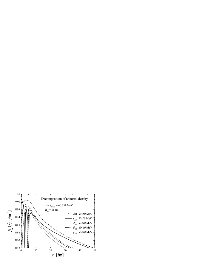
Figure 5: The abnormal density $\tilde{\rho}(r)$ and the contributions from the low-lying resonant states $\tilde{\rho}_{lj}(r)$ obtained by the Woods-Saxon potential plus HFB pairing model in the case of $\lambda$$=$$\varepsilon_{3s_{1/2}}$$=$$-0.052$ MeV. The box size is fixed to be 75 fm.

Figure 6: The box size dependence of $\tilde{\rho}_{s_{1/2}}(r)$ in the case of $\lambda$$=$$\varepsilon_{3s_{1/2}}$$=$$-0.052$ MeV. The results obtained with $R_{box}=$ 30, 75, and 400 fm are compared.

In the present subsection, we discuss the pairing correlation in loosely-bound nuclei. We focus on the applicability of HFB calculation with the box boundary condition for the extreme situation; the pairing effect on the $s_{1/2}$ state in the limit of $\varepsilon_{s_{1/2}}\to 0$. In Fig.1 the average pairing gap and the pairing energy around ⁸⁶Ni are plotted as a function of $\lambda=\varepsilon_{3s_{1/2}}$. The single-particle energy changes by varying $V_{WS}$ while keeping the other parameters fixed. The box boundary condition with $R_{box}=75$ fm is imposed. Pairing correlation becomes monotonically stronger as $\varepsilon_{3s_{1/2}}$ increasing up to around -0.5 MeV, because of the change of the shell structure that is self-consistently taken into account in the pairing potential. The pairing correlation is much enhanced in the very loosely-bound region, $\lambda=\varepsilon_{3s_{1/2}}$ $>$ $-0.5$ MeV, due to the increasing coupling to the nearby continuum BD99 . The importance of the coupling to the non-resonant continuum states for pairing correlation is also discussed in connection with di-neutron correlation MM04 .

To examine whether such enhancement of pairing correlation is due to the artifact of the box boundary condition, we examined the box size dependence up to $R_{box}=400$ fm. In Fig.2 the pairing energy in the case of $\lambda=\varepsilon_{3s_{1/2}}=-0.052$ MeV is shown as a function of $R_{box}$. The strength $V_{WS}$ is fixed to be -39.0 MeV. We confirm that the box size 75 fm is enough to describe the pairing correlation in such very loosely-bound nuclei.

To estimate the pairing effect in the $3s_{1/2}$ state, Hamamoto et al. HS04 introduced the effective pairing gap by $\Delta_{eff}(s_{1/2})\equiv E_{s_{1/2}}$, where the smallest quasiparticle energy $E_{s_{1/2}}$ is calculated with the condition $\lambda=\varepsilon_{3s_{1/2}}$ for the discrete state satisfying $(\lambda+E_{s_{1/2}})<0$. In the case of $(\lambda+E_{s_{1/2}})>0$, the value of $E_{s_{1/2}}$ is obtained by calculating the derivative of the phase sift of the quasiparticle wave function $u_{s_{1/2}}(E_{s_{1/2}},r)$. In our analysis, to estimate the average pairing effect on the resonant state, we introduce the average effective pairing gap by

$$\Delta_{eff}(s_{1/2})=E_{av}(s_{1/2}),$$ (20)

where $E_{av}(s_{1/2})$ is the average energy of the resonant state with the occupation probability,

$$E_{av}(s_{1/2}) = \frac{1}{N_{res}(s_{1/2})}$$ (21)

$$\times\sum_{n}\theta(E_{s_{1/2},n}<10)(v_{s_{1/2},n})^{2}E_{s_{1/2},n},$$

where $\theta(x<a)=$1 for $x<a$, otherwise 0. The occupation probability at $E_{lj,n}$ is defined by

$$(v_{lj,n})^{2}=\int_{0}^{R_{box}}\{v_{lj}(E_{lj,n},r)\}^{2}dr.$$ (22)

The integrated occupation probability over the resonant state,

$$N^{(res)}_{lj}=\sum_{n}\theta(E_{lj,n}<10)(v_{lj,n})^{2},$$ (23)

is introduced.

In Fig.3 $\Delta_{eff}(s_{1/2})$ is plotted as a function of $\lambda=\varepsilon_{3s_{1/2}}$. As $\lambda=\varepsilon_{3s_{1/2}}$ increases, $\Delta_{eff}(s_{1/2})$ monotonically increases. The enhancement of $\Delta_{eff}(s_{1/2})$ in the limit of $\lambda=\varepsilon_{3s_{1/2}}\to 0$ appears. This behavior is consistent with the pairing correlation of the total system measured by $\bar{\Delta}$ and $E_{pair}$ (see Fig.1). This means that the strong coupling between the pairing potential and the $s_{1/2}$ state remains in the limit of $\lambda=\varepsilon_{3s_{1/2}}\to 0$.

We also examined the box size dependence of $\Delta_{eff}(s_{1/2})$. In Fig.4 the occupation probability of the $s_{1/2}$ state in the case of $\lambda=\varepsilon_{3s_{1/2}}=-0.052$ MeV is shown as a function of $E_{s_{1/2}}$. The results obtained with $R_{box}=$ 75 and 400 fm are compared. Although the level density of the discretized continuum states is very different, the average structure of the resonance is unchanged. Namely the integrated occupation probability $N^{(res)}_{s_{1/2}}$ is 0.430 (0.429), and the average effective pairing gap $\Delta_{eff}(s_{1/2})$ is 1.15 (1.13) MeV with $R_{box}=75$ (400) fm. And also, as we will discuss in the next subsection, the average root-mean-square (rms) radius of the lower component of the $s_{1/2}$ state is independent of $R_{box}$ larger than 50 fm (see Fig.2).

To emphasize the importance of self-consistency in the pairing potential, we perform HFB calculation with the analytic surface-type pairing potential HM03 ,

$$\Delta(r)\varpropto r\frac{df(r)}{dr},$$ (24)

where $f(r)$ is the Woods-Saxon type function of Eq.(12). The average pairing gap with the analytic potential is defined by

$$\bar{\Delta}=\frac{\int_{0}^{R_{box}}\Delta(r)f(r)r^{2}dr}{\int_{0}^{R_{box}}f(r)r^{2}dr}.$$ (25)

In Fig.3 the average effective pairing gap $\Delta_{eff}(s_{1/2})$ obtained by HFB with the analytic pairing potentials of $\bar{\Delta}=1.0$ and $1.5$ MeV are also shown. These $\Delta_{eff}(s_{1/2})$ decrease rapidly in the limit of zero binding energy, due to the decoupling between the $s_{1/2}$ state and the pairing potential as discussed in Ref.HM04 , contrary to the HFB calculation with the self-consistent pairing potential.

The low-lying $s_{1/2}$ state is the dominant component of $\tilde{\rho}(r)$ outside the surface region in the HFB calculation with the self-consistent pairing potential. To see this, we define the contributions from the low-lying resonant states to $\tilde{\rho}(r)$ by

$$\tilde{\rho}_{lj}(r) = -\frac{(2j+1)}{4\pi r^{2}}\sum_{n}\theta(E_{lj,n}<10)$$ (26)

$$\quad\times u_{lj}(E_{lj,n},r)v_{lj}(E_{lj,n},r).$$

In Fig.5, $\tilde{\rho}_{lj}(r)$ are shown in the case of $\lambda=\varepsilon_{3s_{1/2}}=-0.052$ MeV with $R_{box}=75$ fm. As clearly seen, the $\tilde{\rho}_{s_{1/2}}(r)$ has a sizable component outside the surface region, $r>10$ fm. In Fig.6 the box size dependence of $\tilde{\rho}_{s_{1/2}}(r)$ is examined, and we confirmed that $R_{box}=$ 75 fm is enough to describe the pairing correlations in such very loosely-bound nuclei. Because of the spatially extended component in the self-consistent pairing potential, the pairing field can act on the $s_{1/2}$ state, although the loosely-bound $s_{1/2}$ state is spatially extended. The coupling between the self-consistent pairing potential and the loosely-bound $s_{1/2}$ state becomes much stronger by repeating the process self-consistently because of the pairing anti-halo effect that we will discuss in the next subsection. On the other hand, this process is absent in the analytic pairing potential, and the coupling to the loosely-bound $s_{1/2}$ state becomes artificially weaker for $\varepsilon_{3s_{1/2}}\to 0$.

The enhanced pairing energy in the very loosely-bound nuclei originates from the spatially extended component of $\tilde{\rho}(r)$. As shown in Fig.2 the pairing energy in the case of $\lambda=\varepsilon_{3s_{1/2}}=-0.052$ MeV obtained with $R_{box}=400$ (30) fm is -20.368 (-20.238) MeV. The difference 130 keV is due to the spatially extended component of $\tilde{\rho}(r)$ shown in Fig.6.

II.4 Pairing anti-halo effect in lower components

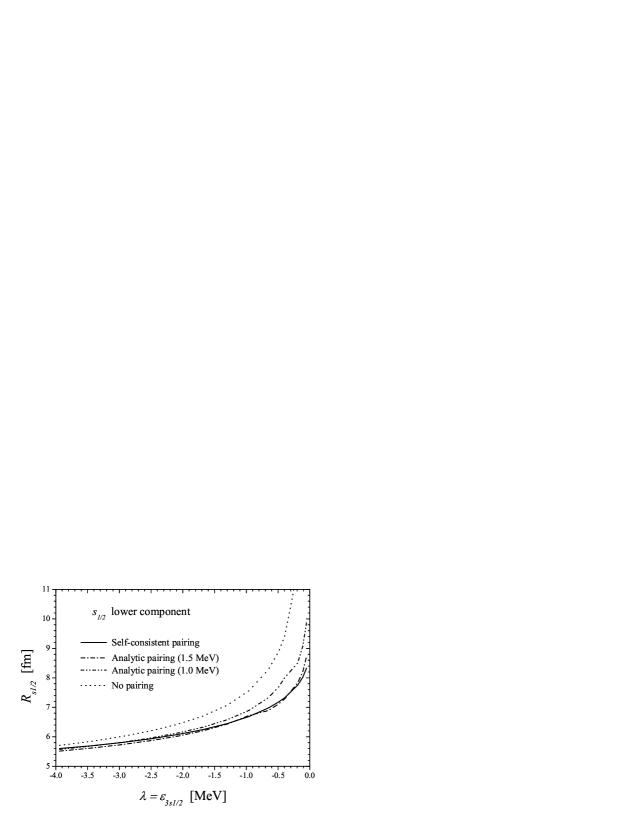
Figure 7: The average rms radius of the lower component of the $s_{1/2}$ quasiparticle wave function as a function of $\lambda$$=$$\varepsilon_{3s_{1/2}}$ obtained by the Woods-Saxon potential plus HFB pairing model. The results with the self-consistent pairing potential and the analytic pairing potentials of $\bar{\Delta}=1.0$ and $1.5$ MeV are compared. The radius without pairing is also shown. The box size is fixed to be 75 fm.

Table 1: The quasiparticle energies of the low-lying resonant states $E^{(res)}_{lj}$ obtained by the Woods-Saxon potential plus HFB pairing model with $V_{WS}=-41.4$ MeV. The average rms radii of the lower components $R_{lj}$ and the integrated occupation probabilities $N^{(res)}_{lj}$ and $N_{lj}(1.0)$ are shown. The single-particle energies of the corresponding bound or resonant states $\varepsilon_{lj}$ are also listed. The box size is fixed to be 75 fm.

	$E^{(res)}_{lj}$ (MeV)	$R_{lj}$ (fm)	$N^{(res)}_{lj}$	$N_{lj}(1.0)$	$\varepsilon_{lj}$ (MeV)
$s_{1/2}$	0.80	7.18	0.48	0.37	-0.50
$d_{3/2}$	1.25	6.12	0.26	0.22	0.14
$d_{5/2}$	1.72	5.79	0.86	0.83	-1.77
$g_{7/2}$	2.05	5.38	0.13	0.13	0.98

Figure 8: The effective hole wave functions of the $s_{1/2}$, $d_{3/2}$, $d_{5/2}$ and $g_{7/2}$ resonant states obtained by the Woods-Saxon potential plus HFB pairing model are shown. The functions in the resonant BCS approximation are also plotted. The strength $V_{WS}=-41.4$ MeV and the box size $R_{box}=75$ fm are fixed.

Self-consistent pairing correlation in HFB has a unique role that changes the spatial structure of the quasiparticle wave functions in loosely-bound nuclei. In the present subsection, we focus on the spatial structure of the lower component, and the structure of the upper component will be discussed in the next subsection.

According to the asymptotic HFB equation with $V_{lj}(r,r^{\prime})\to 0$ and $\Delta(r,r^{\prime})\to 0$ in the limit of $r\to\infty$, the lower component of the quasiparticle wave function decays exponentially for any quasiparticle energy $E_{lj}>0$,

$$v_{lj}(E_{lj},r)\to\exp(-\beta_{lj}r),$$ (27)

where $\beta_{lj}=\sqrt{2m(E_{lj}-\lambda)/\hbar^{2}}$. The HFB quasiparticle energy $E_{lj}$ is well approximated by the canonical quasiparticle energy, $E_{lj}$ $\simeq$ $E_{lj}^{can}$ $\equiv$ $\sqrt{(\epsilon_{lj}^{can}-\lambda)^{2}+(\Delta_{lj}^{can})^{2}}$, where $\epsilon_{lj}^{can}$ and $\Delta_{lj}^{can}$ are the canonical single-particle energy and the canonical pairing gap of the corresponding state DN96 . This means that $\beta_{lj}$ stays at finite value

$$\beta_{lj}\to\sqrt{2mE_{lj}/\hbar^{2}}\geq\sqrt{2m\Delta_{lj}^{can}/\hbar^{2}}>0$$ (28)

with non-zero $\Delta_{lj}^{can}$ for $\lambda\rightarrow 0$. Therefore self-consistent pairing correlation changes the asymptotic behavior of $v_{lj}(E_{lj},r)$, and especially acts against the development of the infinite rms radius that characterizes the wave functions of $s$ and $p$ states in the limit of vanishing binding energy. This change of the spatial structure in the lower component of the quasiparticle wave function is called ”the pairing anti-halo effect” in Ref.BD00 .

In Fig.7 the average rms radii of the lower component of the $s_{1/2}$ state with the self-consistent pairing potential and the analytic pairing potentials of $\bar{\Delta}$$=$$1.0$ and $1.5$ MeV are shown as a function of $\lambda=\varepsilon_{3s_{1/2}}$. The average rms radius $R_{lj}$ is defined by

$$\left(R_{lj}\right)^{2}=\frac{1}{N^{(res)}_{lj}}\sum_{n}\theta(E_{lj,n}<10)$$

$$\qquad\quad\times\int_{0}^{R_{box}}r^{2}\{v_{lj}(E_{lj,n},r)\}^{2}dr.$$ (29)

The radius of the $3s_{1/2}$ state without pairing goes to infinity for $\varepsilon_{3s_{1/2}}\to 0$. On the other hand, the divergence is suppressed in HFB. For $\lambda=\varepsilon_{3s_{1/2}}<-1.5$ MeV, irrespective of the pairing potential, the radii obtained by the HFB calculations have a similar behavior. As approaching the zero binding energy, the spatial structure of the lower component becomes sensitive to the treatment of pairing correlation in accordance with the behavior of the average effective pairing gap $\Delta_{eff}(s_{1/2})$ shown in Fig.3.

In connection with the spatial structure of two-quasiparticle states, we examine the effective hole wave function of the transition with multipolarity $L$ defined by

$$f_{lj,n}^{(L)}(r)=r^{L}v_{lj}(E_{lj,n},r)/v_{lj,n}.$$ (30)

The factor $v_{lj,n}(>0)$ is introduced for the normalization. The effective hole wave functions of the $s_{1/2}$, $d_{3/2}$, $d_{5/2}$ and $g_{7/2}$ resonant states with $L=2$ are plotted in Fig.8. The strength $V_{WS}$ is fixed to be -41.4 MeV to simulate the neutron shell structure in ⁸⁶Ni. The properties of these resonant states are summarized in Table.1. In HFB the effective hole wave function is localized according to Eq.(27), irrespective of the corresponding single-particle energy. However the localization depends on $\ell$. The function $f_{s_{1/2}}^{(2)}(r)$ has the large component not only around the surface region, but also the extended region, 10 fm $<r<$ 20 fm. The component in the extended region remains, but becomes smaller in the $d_{3/2}$ and $d_{5/2}$ states, and negligible in the $g_{7/2}$ state. In Subsec.III we will discuss the impact of such spatially extended part of the lower component in connection with the new aspects of low-frequency vibrational excitations in neutron drip line nuclei.

For comparison, we analyze the effective hole wave functions in the resonant BCS approximation. Although the BCS approximation is not well defined for unstable nuclei due to the unphysical neutron gas DF84 , recently the extended version, the resonant BCS approximation, was proposed SL97 ; SG00 ; SG03 ; CM04 . In this approach, resonant states are taken into account for the particle states. Applicability of the resonant BCS method for ground state properties is discussed in Ref.GS01 . In this approximation, the upper and lower components of the quasiparticle wave function are simply proportional to the corresponding single-particle wave function $\varphi_{lj}(\varepsilon_{lj,n},r)$,

$$\begin{array}[]{l}u_{lj}(E_{lj,n},r)=u_{lj,n}^{BCS}\,\varphi_{lj}(\varepsilon_{lj,n},r),\\ v_{lj}(E_{lj,n},r)=v_{lj,n}^{BCS}\,\varphi_{lj}(\varepsilon_{lj,n},r).\\ \end{array}$$ (33)

The quasiparticle energy $E_{lj,n}$ is related to the single-particle energy $\varepsilon_{lj,n}$ by

$$E_{lj,n}=\sqrt{(\varepsilon_{lj,n}-\lambda)^{2}+(\Delta_{lj,n})^{2}},$$ (34)

where the Fermi energy $\lambda$ and the pairing gap $\Delta_{lj,n}$. $v_{lj,n}^{BCS}$ ($u_{lj,n}^{BCS}$) is the occupation (unoccupation) amplitude. The index $n$ runs over not only the bound states but also the resonant states. For $r\to\infty$, the radial single-particle wave function of the bound state decays exponentially,

$$\varphi_{lj}(\varepsilon_{lj,n},r)\to\exp(-\alpha_{lj,n}r),$$ (35)

where $\alpha_{lj,n}=\sqrt{-2m\varepsilon_{lj,n}/\hbar^{2}}$. On the other hand, the wave function in the continuum region satisfies the scattering boundary condition,

$$\varphi_{lj}(\varepsilon_{lj},r) \to \left[\cos(\delta_{lj})rj_{l}(k_{lj}r)-\sin(\delta_{lj})rn_{l}(k_{lj}r)\right]$$ (36a)

$$\sim \sin(k_{lj}r+\delta^{\prime}_{lj})$$ (36b)

where $k_{lj}=\sqrt{2m\varepsilon_{lj}/\hbar^{2}}$. $j_{l}$ and $n_{l}$ are spherical Bessel and Neumann functions, and $\delta_{lj}$ ($\delta^{\prime}_{lj}\equiv\delta_{lj}-l\pi/2$) is the phase shift corresponding to the angular momentum $(lj)$.

As shown in Fig.8, the effective hole wave functions of the $d_{3/2}$ and $g_{7/2}$ resonant states in the resonant BCS approximation diverge for $r\to\infty$ in contrast with those in HFB. The effective hole wave functions of the bound single-particle states in the (resonant) BCS approximation are essentially the same with those without pairing. The function for the halo state, $f_{s_{1/2}}^{(2)}(r)$, is spatially very extended due to the absence of the pairing anti-halo effect. On the other hand, $f_{d_{5/2}}^{(2)}(r)$ has almost the same spatial structure with that in HFB, because the corresponding single-particle state is the bound state without halo.

II.5 Broadening effect in upper components

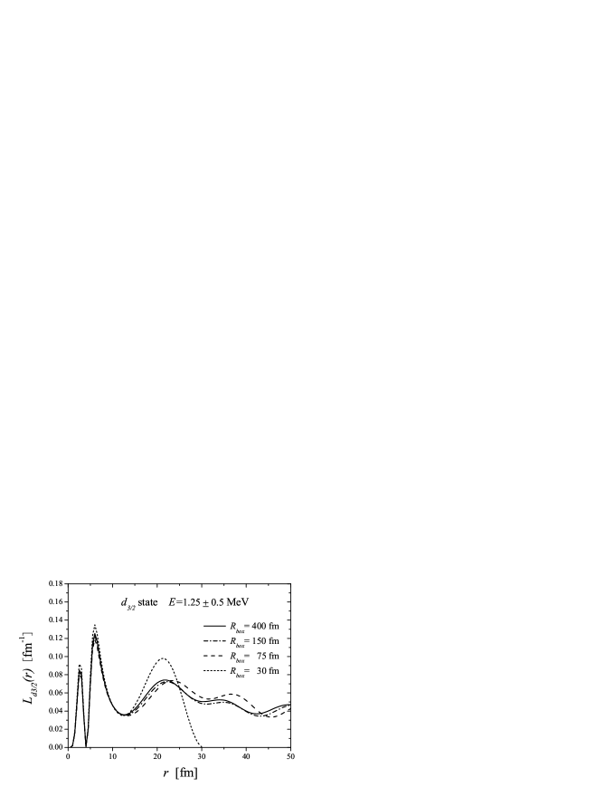
Figure 9: The localization indicator of the resonant $d_{3/2}$ state at $E^{(res)}=1.25$ MeV in the Woods-Saxon potential plus HFB pairing model is shown. The results obtained with $R_{box}=$ 30, 75, 150, and 400 fm are compared.

Figure 10: The localization indicators of the resonant $d_{3/2}$ state at $E^{(res)}=1.25$ MeV and the resonant $g_{7/2}$ state at $E^{(res)}=2.05$ MeV in the Woods-Saxon potential plus HFB pairing model are shown. The ”BCS” localization indicators of the corresponding states are also plotted. The box size is fixed to be 75 fm.

Figure 11: The same as Fig.10 but for the resonant $s_{1/2}$ state at $E^{(res)}$=0.80 MeV and the resonant $d_{5/2}$ state at $E^{(res)}$=1.72 MeV.

Self-consistent pairing correlation also changes the spatial structure of the upper component of the quasiparticle wave function. Asymptotic behavior of the upper component depends on the quasiparticle energy DF84 . In the discrete region $(E_{lj,n}+\lambda)<0$, the wave function decays exponentially,

$$u_{lj}(E_{lj,n},r)\to\exp(-\alpha_{lj,n}r),$$ (37)

where $\alpha_{lj,n}=\sqrt{-2m(E_{lj,n}+\lambda)/\hbar^{2}}$. In the continuum region $(E_{lj}+\lambda)>0$, on the other hand,

$$u_{lj}(E_{lj},r) \to \left[\cos\left(\delta_{lj}\right)rj_{l}(k_{lj}r)-\sin\left(\delta_{lj}\right)rn_{l}(k_{lj}r)\right],$$ (38a)

$$\sim \sin(k_{lj}r+\delta^{\prime}_{lj}),$$ (38b)

with $k_{lj}=\sqrt{2m(E_{lj}+\lambda)/\hbar^{2}}$.

In the neutron drip line region with $\lambda\to 0$, all quasiparticle states are in the continuum region. To examine the spatial structure of the upper components, we introduce the localization indicator,

$$L_{lj}(r;\delta E)=\sum_{n}\theta(|E_{lj,n}-E_{lj}^{(res)}|<\delta E/2)\{u_{lj}(E_{lj,n},r)\}^{2}.$$ (39)

The summation is taken around the resonance energy $E_{lj}^{(res)}$ within the energy window $\delta E$. In principle, the localization indicator is independent of $R_{box}$ with arbitrary $\delta E$, if $R_{box}$ is enough large. In Fig.9 the indicator of the $d_{3/2}$ state at $E^{(res)}=1.25$ MeV obtained with $R_{box}$ $=$ 30, 75, 150, and 400 fm are compared. The energy window $\delta E$ is fixed to be 1.0 MeV. Apart from the artifact around the box boundary, these results coincide in good accuracy. The box size $R_{box}=75$ fm is enough for our discussion on the spatial structure of the two-quasiparticle states around ⁸⁶Ni, because it is required to describe the spatial structure of the upper components within 30 fm as seen in Fig.8.

In Fig.10 the indicators of the $d_{3/2}$ state at $E^{(res)}=$1.25 MeV and the $g_{7/2}$ state at $E^{(res)}=$2.05 MeV, that originate from the resonant single-particle states, are shown. The occupation probabilities within the energy window,

$$N_{lj}(\delta E)=\sum_{n}\theta(|E_{lj,n}-E_{lj}^{(res)}|<\delta E/2)(v_{lj,n})^{2},$$ (40)

together with $\delta E=1$ MeV are listed in Table.1. To examine the role of self-consistent pairing correlation, as the reference distribution, the localization indicator in the resonant BCS approximation (we call the ”BCS” localization indicator) for $\varepsilon_{lj}^{(res)}>0$ is introduced by

$$L_{lj}(r;\delta E)=(1-N_{lj}(\delta E))\times$$

$$\quad\sum_{n}\theta(|\varepsilon_{lj,n}-\varepsilon_{lj}^{(res)}|<\delta E/2)\{\varphi_{lj}(\varepsilon_{lj,n},r)\}^{2}.$$ (41)

The single-particle wave function $\varphi_{lj}(\varepsilon_{lj,n},r)$ with $\varepsilon_{lj,n}>0$ is the solution of the Woods-Saxon potential of Eq.(11) with the box boundary condition.

In the $g_{7/2}$ resonant state, the difference between the HFB and ”BCS” indicators is small within 20 fm. On the other hand, in the $d_{3/2}$ state, the spatial localization of the resonance is weakened in HFB; namely, the component within the centrifugal barrier ($r<10$ fm) is reduced, and enhanced in the extended region (10 fm $<r<$ 20 fm). This is the direct manifestation of the strong mixing with the nearby non-resonant continuum states. As discussed in Ref.DF84 ; HM03 ; GS01 ; FT00 , the resonance width of the quasiparticle state originating from the resonant (bound) single-particle state is broadened (acquired) in HFB. This effect is more prominent in lower-$\ell$ states with smaller quasiparticle energy. Consequently, the spatial structure of the upper component of the quasiparticle wave function changes, and the spatial localization is weakened by the mixing with continuum states. To emphasize this effect induced by self-consistent pairing correlation; the broadened resonance width and the spatially weakened localization, we call ”the broadening effect” in the upper component.

In Fig.11 the localization indicators of the $s_{1/2}$ state at $E^{(res)}=0.80$ MeV and the $d_{5/2}$ state at $E^{(res)}=1.72$ MeV, that originate from the bound single-particle states, are shown. The ”BCS” localization indicator with $\varepsilon_{lj,n}<0$ is defined by

$$L_{lj}(r)=(1-N_{lj}(\delta E))\{\varphi_{lj}(\varepsilon_{lj,n},r)\}^{2}.$$ (42)

In these states, the spatial structure of the HFB and ”BCS” indicators is very different. The ”BCS” indicator is localized, but non-localized in HFB, because of the different boundary conditions, and the broadening effect is absent in the (resonant) BCS approximation. The broadening effect is strong in the upper component of the $s_{1/2}$ and $d_{3/2}$ states. Especially the localization around the surface region is strongly affected in the $s_{1/2}$ state.

III Spatial structure of two-quasiparticle states

III.1 Two-quasiparticle states in HFB

The spatial localization of two-quasiparticle states ($1p$-$1h$ states in closed shell nuclei) is a necessary condition to realize the coherent motions among them. In stable nuclei the spatial localization of the contributing two-quasiparticle states is realized around the surface region (for example, see Ref.GM65 ; FP67 ). In neutron drip line nuclei, on the other hand, because the contributing single-particle states are tightly-bound states, loosely-bound states, resonant and non-resonant continuum states, the spatial distributions of the two-quasiparticle states have rich variety of the spatial character. Therefore, first of all, the realization of coherent motions among them is not obvious. If they can be realized, we may expect qualitatively new aspects of low-frequency vibrational excitations in neutron drip line nuclei.

In the present study, we analyze the transitions from the ground state to excited states within the same nucleus. The spatial distribution of the particle-hole component of the two-quasiparticle state between the upper component $u_{l^{\prime}j^{\prime}}(E_{l^{\prime}j^{\prime}},r)$ and the lower component $v_{lj}(E_{lj},r)$ is defined by

$$F_{uv}^{(L)}(r)\equiv u_{l^{\prime}j^{\prime}}(E_{l^{\prime}j^{\prime}},r)r^{L}v_{lj}(E_{lj},r)/N_{uv},$$ (43)

where $N_{uv}$ $=$ $\sqrt{1-(v_{l^{\prime}j^{\prime}})^{2}}v_{lj}$ $(>0)$ is the normalization factor.

One of the novel features of low-frequency vibrational excitations in neutron drip line nuclei is that two-quasiparticle states composed of quasiparticles both in the continuum region are inevitably involved. In HFB, owing to the pairing anti-halo effect, the asymptotic behavior for $r\to\infty$ is,

$$F_{uv}^{(L)}(r)\to r^{L}\sin(k_{l^{\prime}j^{\prime}}r+\delta^{\prime}_{l^{\prime}j^{\prime}})\exp(-\beta_{lj}r).$$ (44)

Since $\beta_{lj}$ stay at finite with non-zero pairing correlation, the spatial distribution is localized irrespective of the quasiparticle energy.

Recently QRPA calculation with the resonant BCS approximation is applied to describe vibrational excitations in loosely-bound nuclei HG04 ; CM05 . In this method, according to Eq.(36b), the spatial distribution of the two-quasiparticle state composed of quasiparticles both in the continuum is non-localized function with the asymptotic behavior,

$$F_{uv}^{(L)}(r) \to r^{L}\sin(k_{l^{\prime}j^{\prime}}r+\delta^{\prime}_{l^{\prime}j^{\prime}})\sin(k_{lj}r+\delta^{\prime}_{lj}).$$ (45)

Consequently the spatial integration, namely the transition matrix element, diverges. In practice this divergence may be suppressed by imposing the box boundary condition with small box size, typically $R_{box}=15$ fm HG04 . However a large box radius is needed to represent the wave functions with the spatially extended structure in good accuracy. Therefore this approximation is uncontrollable for the description of excitations in nuclei close to the neutron drip line. In Ref.CM05 the low-lying dipole modes in ^26,28Ne are studied by means of quasiparticle relativistic RPA with the resonant BCS approximation. In this calculation, although the resonant states are calculated by imposing the scattering boundary condition, the obtained results don’t suffer with the problem of the divergence because of the peculiarity of the shell structure. For example, the two-quasiparticle state between the resonant $f_{7/2}$ and $p_{3/2}$ states doesn’t contribute to the dipole excitation in ²⁸Ne. Moreover the unoccupied states outside of the pairing active space are obtained by expanding on a set of the harmonic oscillator basis, and the divergence of the two-quasiparticle states between the occupied part of the resonant states and the non-resonant continuum states is artificially eliminated.

III.2 Broad localization of two-quasiparticle states

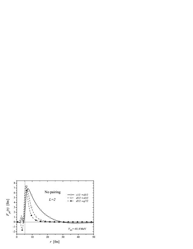
Figure 12: The $F_{ph}^{(2)}(r)$ between the bound states and the resonant states with $\varepsilon_{p}$$-$$\varepsilon_{h}$$<$$5$ MeV in ⁸⁶Ni.

Figure 13: The first moments $R_{ph}^{(2)}$ of $F_{ph}^{(2)}(r)$ in Fig.12. The regions $|R_{ph}^{(2)}-r|<\sigma_{ph}^{(2)}$ are shown by vertical line segments.

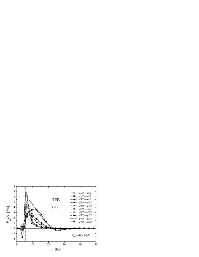
Figure 14: The $F_{uv}^{(2)}(r)$ associated with the low-lying $s_{1/2}$, $d_{3/2}$, $d_{5/2}$, and $g_{7/2}$ resonant states in ⁸⁶Ni obtained by the Woods-Saxon potential plus HFB pairing model.

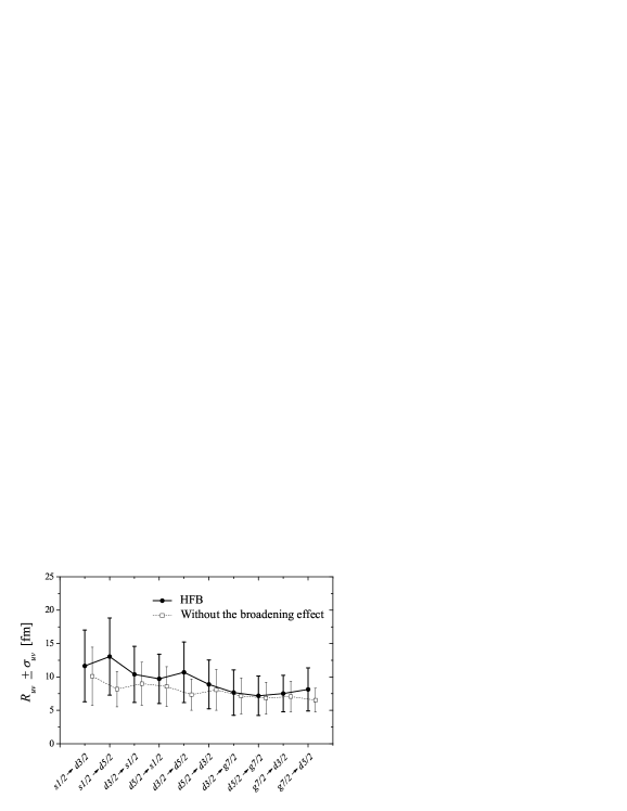
Figure 15: The first moments $R_{uv}^{(2)}$ of $F_{uv}^{(2)}(r)$ in Fig.14. The regions $|R_{uv}^{(2)}-r|<\sigma_{uv}^{(2)}$ are shown by vertical line segments. The result without the broadening effect in the upper components of the quasiparticle wave functions is also shown.

As the illustrative example of neutron drip line nuclei, we examine the spatial structure of the neutron quadrupole two-quasiparticle states in ⁸⁶Ni. To characterize the spatial structure of $F_{uv}^{(L)}(r)$, we introduce the first moment,

$$R_{uv}^{(L)}=\frac{\int_{0}^{R_{box}}r|F_{uv}^{(L)}(r)|dr}{\int_{0}^{R_{box}}|F_{uv}^{(L)}(r)|dr},$$ (46)

and the variance,

$$\left(\sigma_{uv}^{(L)}\right)^{2}=\frac{\int_{0}^{R_{box}}r^{2}|F_{uv}^{(L)}(r)|dr}{\int_{0}^{R_{box}}|F_{uv}^{(L)}(r)|dr}-\left(R_{uv}^{(L)}\right)^{2}.$$ (47)

If the regions $|R_{uv}^{(L)}-r|<\sigma_{uv}^{(L)}$ have overlap, we expect the correlations among the two-quasiparticle states.

In Fig.12 the spatial distributions without pairing, $F_{ph}^{(2)}(r)$, are shown. Because the available particle states are only the $d_{3/2}$ and $g_{7/2}$ resonant states, the $1p$-$1h$ excitations to the resonant states with $\varepsilon_{p}-\varepsilon_{h}<5$ MeV are (a) $3s_{1/2}$ $\to$ resonant $d_{3/2}$, (b) $2d_{5/2}$ $\to$ resonant $d_{3/2}$, and (c) $2d_{5/2}$ $\to$ resonant $g_{7/2}$. The corresponding $R_{ph}^{(2)}$ and the regions $|R_{ph}^{(2)}-r|<\sigma_{ph}^{(2)}$ are shown in Fig.13. These configurations have overlap around the surface region, and the correlations among them bring some low-lying collectivity. However the lowest $1p$-$1h$ state (a) only have the appreciable component outside the surface region that can’t correlate with the other configurations, and the lowest RPA solution becomes a single-particle like excitation as we will discuss in Subsec.IV.2.

In Fig.14 the spatial distribution of the two-quasiparticle states associated with the low-lying $s_{1/2}$, $d_{3/2}$, $d_{5/2}$ and $g_{7/2}$ resonant states are plotted. Due to the pairing anti-halo effect, all distribution functions are localized in HFB. The corresponding $R_{uv}^{(2)}$ and the regions $|R_{uv}^{(2)}-r|<\sigma_{uv}^{(2)}$ are shown in Fig.15. The distributions of the two-quasiparticle states between the $s_{1/2}$, $d_{3/2}$ and $d_{5/2}$ resonant states have the sizable components in the spatially extended region around 10 fm $<r<$ 15 fm, in addition to the surface region where the localization is achieved in stable nuclei. Because of the spatially extended structure, the transition matrix elements can be larger than those of the tightly bound states in stable nuclei. Therefore we can expect the large collectivity of low-frequency vibrational excitations by the spatially extended coherence among the two-quasiparticle states. We call such spatially extended distribution of the two-quasiparticle states ”the broad localization”.

In Figs.14 and 15 the spatial structure of the two-quasiparticle states involving the $g_{7/2}$ resonant state is also shown. Because the upper and lower components of the $g_{7/2}$ quasiparticle state are strongly confined within the centrifugal barrier, the $F_{uv}^{(2)}(r)$ concentrate only around the surface region. In general, we can expect the large collectivity by the broad localization with low-$\ell$ neutrons, and the effect is weaker in the two-quasiparticle states involving larger-$\ell$ states.

The broad localization is realized owing to the broadening effect in the upper component of the quasiparticle wave function. For comparison, the $R_{uv}^{(2)}$ and the regions $|R_{uv}^{(2)}-r|<\sigma_{uv}^{(2)}$ without the broadening effect, that are calculated with the lower components obtained by HFB and the upper components obtained by the resonant BCS approximation, are shown in Fig.15. If the broadening effect is absent, the distributions concentrate only around the surface region with small $\sigma_{uv}^{(2)}$. In this situation, the collective motions among them can appear, however the low-frequency vibrational excitations have a similar behavior with those in stable nuclei, and novel features of neutron drip line nuclei are suppressed.

IV HFB plus QRPA calculation

IV.1 Formulation and inputs

We consider the first $2^{+}$ states in neutron rich Ni isotopes to examine the unique role of self-consistent pairing correlation in the neutron drip line nuclei. In Fig.16 the neutron single-particle energies obtained by HF calculation with Skyrme SLy4 force CB98 are shown. The neutron drip line nucleus is ⁸⁶Ni within the HF calculation. By taking into account pairing correlations, more neutrons can bound. However the predicted position of the neutron drip line depends on the treatment of pairing correlations, for example, the drip line nucleus is ⁸⁸Ni in Ref.GS01 and ⁹²Ni in Ref.MD00 . The predicted drip line also depends on the effective interactions and the frameworks; namely relativistic or non-relativistic approaches (for example, see Ref.MD00 ; Me98 ). In the present study we consider up to ⁸⁸Ni, because our purpose is to investigate the qualitative aspects of vibrational excitations in neutron drip line nuclei.

We perform HFB plus QRPA calculation with Skyrme force. The HFB mean fields are determined self-consistently from an effective force and the residual interaction of the QRPA problem is derived from the same force. The QRPA problem is solved by the response function method in coordinate space. A detailed account of the method can be found in Ref.YG04 ; YK03 ; KS02 . The residual interaction has an explicit momentum dependence, and these momentum dependence are explicitly treated in our QRPA calculations. Because we calculate only natural parity (non spin-flip) excitations, we drop the spin-spin part of the residual interaction. The residual Coulomb and residual spin-orbit interactions are also dropped.

The ground states are obtained by Skyrme-HFB calculation. The HFB equation is diagonalized on a Skyrme-HF basis represented in coordinate space with the box boundary condition of $R_{box}=30$ fm. Spherical symmetry is imposed on the quasiparticle wave functions. The quasiparticle states with the energy below 50 MeV and the orbital angular momentum up to $7\hbar$ are taken into account. The Skyrme SLy4 force is used for the HF mean-field. The density-dependent zero-range pairing interaction of Eq.(13) with the density $\rho(r)$ of protons plus neutrons is adopted for the pairing field. The parameters are taken to be $V_{pair}=-555$ MeV fm^-3 and $\rho_{c}=0.16(\approx\rho(0))$ fm^-3, that give the average neutron pairing gap $\bar{\Delta}_{n}\approx 12/\sqrt{86}$ in ⁸⁶Ni.

IV.2 First $2^{+}$ states in Ni isotopes

Figure 16: The neutron single-particle energies in neutron rich Ni isotopes obtained by HF with Skyrme SLy4 force. The approximate resonance energies with $R_{box}=30$ fm are also shown. The neutron Fermi energies in HFB are indicated by thick line.

Figure 17: The $B(E2,0^{+}_{1}\rightarrow 2^{+}_{1})$ values and the excitation energies of the first $2^{+}$ states in neutron rich Ni isotopes obtained by HFB plus QRPA, resonant BCS plus QRPA, and RPA with Skyrme SLy4 force.

Figure 18: The box size dependence of the $B(E2)$ values obtained by HFB plus QRPA with Skyrme SLy4 force.

Figure 19: The isoscalar and charge quadrupole strength functions in ⁸⁶Ni obtained by HFB plus QRPA with Skyrme SLy4 force. The corresponding unperturbed strengths are also shown. A width parameter $\Gamma=0.05$ MeV is introduced for the plots. The threshold energy $E_{th}$ is indicated by arrow.

Figure 20: The isoscalar and charge quadrupole strength functions in ⁸⁶Ni obtained by RPA with Skyrme SLy4 force. The corresponding unperturbed strengths are also shown. The neutron $1p$-$1h$ excitations; (a) $3s_{1/2}$ $\to$ resonant $d_{3/2}$, (b) $2d_{5/2}$ $\to$ resonant $d_{3/2}$, and (c) $2d_{5/2}$ $\to$ resonant $g_{7/2}$, are indicated by vertical lines. The configuration, (x) $3s_{1/2}$ $\to$ (discretized) non-resonant continuum $d_{5/2}$, is also pointed out. A width parameter $\Gamma=0.05$ MeV is introduced for the plots. The threshold energy $E_{th}$ is indicated by arrow.

In Fig.17 the $B(E2,0^{+}_{1}\rightarrow 2^{+}_{1})$ values and the excitation energies of the first $2^{+}$ states in neutron rich Ni isotopes obtained by HFB plus QRPA calculation are shown. These $2^{+}$ states are discrete solutions below the threshold energies. The $B(E2)$ values increase as approaching the neutron drip line. The $B(E2)$ values in the single-particle unit (=5 times the Weisskopf unit) are 7.8 in ⁸⁶Ni, and 11.7 in ⁸⁸Ni. To examine the convergence of the solutions, the box size dependence of the $B(E2)$ values is shown in Fig.18. Because the spatial distribution of the contributing two-quasiparticle states is localized by the pairing anti-halo effect, the coherence among them occurs within 20 fm as shown in Fig.15. Therefore $R_{box}=20$ fm is enough for the convergence.

In Fig.19 the isoscalar and charge quadrupole response functions in ⁸⁶Ni obtained by HFB plus QRPA, and the corresponding unperturbed strength functions are shown. For the plots, a small width parameter of $\Gamma=0.05$ MeV is introduced. All two-quasiparticle states are in the continuum region, and the configurations below 6 MeV are of neutrons except for the proton $(2p_{3/2})(1f_{7/2})^{-1}$ configuration at 4.9 MeV. The strong coherence among the neutrons, and the successive isoscalar coherent motion of protons and neutrons lead to the large $B(E2)$ value.

To examine the role of self-consistent pairing correlation, the results of the resonant BCS plus QRPA calculation up to ⁸⁶Ni are also plotted in Fig.17. Although the resonant BCS approximation is not well-defined in neutron drip line region, the results are shown to emphasize the limited applicability of this approximation. The technical detail of our resonant BCS plus QRPA calculation is explained in the previous report Ya04 . The box size of $R_{box}=20$ fm is used only for the resonant BCS approximation. The results have the smooth dependence on $R_{box}$ up to around 20 fm, and they are consistent with our preliminary results obtained by the resonant BCS plus QRPA calculation with the constant pairing gap approximation Ya04 . However we couldn’t obtain the regular solution in ^84,86Ni with the larger $R_{box}$. In the present study, as an improvement, the density-dependent pairing interaction of Eq.(13) is used. Because the cut-off energies of the particle model space are different in the resonant BCS calculation and the QRPA calculation, the different pairing strengths must be used for them. The pairing strength is changed for each nucleus to reproduce the average neutron pairing gap obtained by HFB calculation. On the other hand, for the QRPA residual interaction, exactly the same interaction used in the HFB plus QRPA calculation is adopted.

From ⁸⁰Ni to ⁸²Ni, the results of the HFB plus QRPA and the resonant BCS plus QRPA have a similar behavior; namely the energies decrease and the $B(E2)$ values increase. On the other hand, as approaching the neutron drip line, the $B(E2)$ values obtained by the resonant BCS plus QRPA calculation are much smaller than those in the HFB plus QRPA calculation. The main qualitative difference between these calculations is the realization of the broad localization of the two-quasiparticle states associated with the neutron low-lying $s_{1/2}$, $d_{3/2}$ and $d_{5/2}$ resonant states in HFB.

The results for ^84,86Ni obtained by RPA calculation are also shown in Fig.17. The $B(E2)$ values in RPA is much smaller than those in the resonant BCS plus QRPA calculation, because the contributions of the hole-hole channel can increase the collectivity of these excitations. As we have discussed in Subsec.III.2, the lowest discrete solutions in RPA are single-particle like excitations. The excitation energies are almost the same with the specific $1p$-$1h$ energies ($2d_{5/2}$ $\to$ $3s_{1/2}$ in ⁸⁴Ni, and $3s_{1/2}$ $\to$ resonant $d_{3/2}$ in ⁸⁶Ni). In Fig.20 the isoscalar and charge quadrupole strengths in ⁸⁶Ni obtained by RPA calculation, and the corresponding unperturbed strengths are shown. The neutron $1p$-$1h$ excitations; (a) $3s_{1/2}$ $\to$ resonant $d_{3/2}$, (b) $2d_{5/2}$ $\to$ resonant $d_{3/2}$, and (c) $2d_{5/2}$ $\to$ resonant $g_{7/2}$, are indicated. The excitation, (x) $3s_{1/2}$ $\to$ (discretized) non-resonant continuum $d_{5/2}$, is also pointed out.

The excitations to the resonant states, (a), (b) and (c), can generate some collectivity among the localized components (see Figs.12 and 13). However the $B(E2)$ values of the first 2⁺ states in RPA change from 234 $e^{2}$fm⁴ to 173 $e^{2}$fm⁴ in ⁸⁴Ni, from 83.0 $e^{2}$fm⁴ to 74.5 $e^{2}$fm⁴ in ⁸⁶Ni as increasing the box size from 20 fm to 30 fm. The HF calculation with small $R_{box}$ leads to the artificial localization of the spatially extended wave functions. Accordingly the RPA calculation overestimates the correlations among these $1p$-$1h$ states. To obtain fully convergent solutions in RPA, much larger $R_{box}$ or continuum RPA calculation is required. The excitations to non-resonant continuum states like (x) can’t produce the collectivity. The small peak related to (x) in the charge quadrupole strength is an artifact of the box boundary condition, and the strength decreases with larger $R_{box}$.

V Conclusion

We have investigated the role of low-$\ell$ neutrons and pairing correlations for low-frequency vibrational excitations in neutron drip line nuclei. We have clarified the change of the spatial structure of quasiparticle wave functions induced by self-consistent pairing correlation; the pairing anti-halo effect in the lower component and the broadening effect in the upper component. We have found that the broad localization of two-quasiparticle states among low-$\ell$ neutrons is realized in consequence of the structure change in the quasiparticle wave functions. The broad localization can cause novel features of low-frequency vibrational excitations in nuclei close to the neutron drip line; as demonstrated by HFB plus QRPA calculation for the first 2⁺ states in neutron rich Ni isotopes, it brings about the spatially extended coherence and the large transition strength.

- (1) P. Ring, and P. Schuck, The Nuclear Many-Body Problem (Springer-Verlag, Berlin, 1980).
- (2) A. Mueller and B. Sherril, Annu. Rev. Nucl. Part. Sci. 43, 529 (1993).
- (3) K. Riisager, Rev. Mod. Phys. 66, 1105 (1994).
- (4) P.G. Hansen, A.S. Jensen, and B. Jonson, Annu. Rev. Nucl. Part. Phys. 45, 591 (1995).
- (5) I. Tanihata, Jour. of Phys. G 22, 157 (1996).
- (6) A. S. Jensen, K. Riisager, D. V. Fedorov, and E. Garrido, Rev. Mod. Phys. 76, 215 (2004).
- (7) H. Sagawa, N.Van Giai, N. Takigawa, M. Ishihara, and K. Yazaki, Z.Phys. A 351, 385 (1995).
- (8) D. Sackett, K. Ieki, A. Galonsky, C. A. Bertulani, H. Esbensen, J. J. Kruse, W. G. Lynch, D. J. Morrissey, N. A. Orr, B. M. Sherrill, H. Schulz, A. Sustich, J. A. Winger, F. Deák, Á. Horváth, and Á. Kiss, Z. Seres, J. J. Kolata, R. E. Warner, D. L. Humphrey, Phys. Rev. C 48, 118 (1993).
- (9) S. Shimoura, T. Nakamura, M. Ishihara, N. Inabe, T. Kobayashi, T. Kubo, R. H. Siemssen, I. Tanihata and Y. Watanabe, Phys. Lett. B348, 29 (1995).
- (10) M. Zinser, F. Humbert, T. Nilsson, W. Schwab, H. Simon, T. Aumann, M. J. G. Borge, L. V. Chulkov, J. Cub, Th. W. Elze, H. Emling, H. Geissel, D. Guillemaud-Mueller, P. G. Hansen, R. Holzmann, H. Irnich, B. Jonson, J. V. Kratz, R. Kulessa, Y. Leifels, H. Lenske, A. Magel, A. C. Mueller, G. Münzenberg, F. Nickel, G. Nyman, A. Richter, K. Riisager, C. Scheidenberger, G. Schrieder, K. Stelzer, J. Stroth, A. Surowiec, O. Tengblad, E. Wajda, E. Zude, Nucl. Phys. A619, 151 (1997).
- (11) T. Nakamura, S. Shimoura, T. Kobayashi, T. Teranishi, K. Abe, N. Aoi, Y. Doki, M. Fujimaki, N. Inabe, M. Iwasa, K. Katori, T. Kubo, H. Okuno, T. Suzuki, I. Tanihata, Y. Watanabe, A. Yoshida, M. Ishihara, Phys. Lett. B331, 296 (1994).
- (12) R. Palit, P. Adrich, T. Aumann, K. Boretzky, B. V. Carlson, D. Cortina, U. Datta Pramanik, Th. W. Elze, H. Emling, H. Geissel, M. Hellström, K. L. Jones, J. V. Kratz, R. Kulessa, Y. Leifels, A. Leistenschneider, G. Münzenberg, C. Nociforo, P. Reiter, H. Simon, K. Sümmerer, and W. Walus, Phys. Rev. C 68, 034318 (2003).
- (13) T. Nakamura, N. Fukuda, T. Kobayashi, N. Aoi, H. Iwasaki, T. Kubo, A. Mengoni, M. Notani, H. Otsu, H. Sakurai, S. Shimoura, T. Teranishi, Y. X. Watanabe, K. Yoneda, and M. Ishihara, Phys. Rev. Lett. 83, 1112 (1999).
- (14) U. Datta Pramanik, T. Aumann, K. Boretzky, B. V. Carlson, D. Cortina, Th. W. Elze, H. Emling, H. Geissel, A. Grünschloß, M. Hellström, S. Ilievski, J. V. Kratz, R. Kulessa, Y. Leifels, A. Leistenschneider, E. Lubkiewicz, G. Münzenberg, P. Reiter, H. Simon, K. Sümmerer, E. Wajda and W. Walus Phys. Lett. B551, 63 (2003).
- (15) T. Aumann, D. Aleksandrov, L. Axelsson, T. Baumann, M. J. G. Borge, L. V. Chulkov, J. Cub, W. Dostal, B. Eberlein, Th. W. Elze, H. Emling, H. Geissel, V. Z. Goldberg, M. Golovkov, A. Grünschloß, M. Hellström, K. Hencken, J. Holeczek, R. Holzmann, B. Jonson, A. A. Korshenninikov, J. V. Kratz, G. Kraus, R. Kulessa, Y. Leifels, A. Leistenschneider, T. Leth, I. Mukha, G. Münzenberg, F. Nickel, T. Nilsson, G. Nyman, B. Petersen, M. Pfützner, A. Richter, K. Riisager, C. Scheidenberger, G. Schrieder, W. Schwab, H. Simon, M. H. Smedberg, M. Steiner, J. Stroth, A. Surowiec, T. Suzuki, O. Tengblad, and M. V. Zhukov, Phys. Rev. C 59, 1252 (1999).
- (16) P. G. Hansen, and B. Jonson, Europhys. Lett. 4, 409 (1987).
- (17) K. Ikeda, Nucl. Phys. A538, 355c (1992).
- (18) J. Dobaczewski, H. Flocard, and J. Treiner, Nucl. Phys. A422, 103 (1984).
- (19) A. Bulgac, preprint No. FT-194-1980, Institute of Atomic Physics, Bucharest, 1980, (nucl-th/9907088).
- (20) S. T. Belyaev, A. V. Smirnov, S. V. Tolokonnikov, and S. A. Fayans, Yad. Fiz. 45, 1263 (1987).
- (21) J. Dobaczewski, W. Nazarewicz, T. R. Werner, J. F. Berger, C. R. Chinn, and J. Dechargé, Phys. Rev. C 53, 2809 (1996).
- (22) I. Hamamoto, and B. R. Mottelson, Phys. Rev. C 68, 034312 (2003).
- (23) I. Hamamoto, H. Sagawa, Phys. Rev. C 70, 034317 (2004).
- (24) I. Hamamoto, and B. R. Mottelson, Phys. Rev. C 69, 064302 (2004).
- (25) E. Chabanat, P. Bonche, P. Haensel, J. Meyer, and R. Schaeffer Nucl. Phys. A635, 231 (1998); Erratum Nucl. Phys. A643, 441 (1998).
- (26) K. Bennaceur, J. Dobaczewski, and M. Ploszajczak, Phys. Rev. C 60, 034308 (1999).
- (27) M. Matsuo, K. Mizuyama, and Y. Serizawa, preprint nucl-th/0412062.
- (28) K. Bennaceur, J. Dobaczewski, and M. Ploszajczak, Phys. Lett. B 496, 154 (2000).
- (29) N. Sandulescu, R. J. Liotta, and R. Wyss, Phys. Lett. B 394, 6 (1997).
- (30) N. Sandulescu, Nguyen Van Giai, and R. J. Liotta, Phys. Rev. C 61, 061301 (2000).
- (31) N. Sandulescu, L. S. Geng, H. Toki, and G. C. Hillhouse, Phys. Rev. C 68, 054323 (2003).
- (32) L. -G. Cao, and Z. -Yu. Ma, Eur. Phys. J. A 22, 189 (2004)
- (33) M. Grasso, N. Sandulescu, Nguyen Van Giai, and R. J. Liotta, Phys. Rev. C 64, 064321 (2001).
- (34) S. A. Fayans, S. V. Tolokonnikov, and D. Zawischa, Phys. Lett. B 491, 245 (2000)
- (35) I. M. Green, and S. A. Moszkowski, Phys. Rev. 139, 790 (1965).
- (36) A. Faessler, and A. Plastino, Nucl. Phys. A94, 580 (1967).
- (37) Masayuki Yamagami, in Proceedings of ”the Fifth Japan-China Joint Nuclear Physics Symposium”, Fukuoka, Japan, 2004, edited by Y. Gono, N. Ikeda and K. Ogata, p218; preprint nucl-th/0404030.
- (38) K. Hagino, Nguyen Van Giai, and H. Sagawa, Nucl. Phys. A731, 264 (2004).
- (39) Li-G. Cao, Z.-Y. Ma, Phys.Rev. C 71, 034305 (2005).
- (40) S. Mizutori, J. Dobaczewski, G. A. Lalazissis, W. Nazarewicz, and P. -G. Reinhard, Phys. Rev. C 61, 044326 (2000).
- (41) J. Meng, Phys. Rev. C 57, 1229 (1998).
- (42) M. Yamagami, and Nguyen Van Giai, Phys. Rev. C 69, 034301 (2004).
- (43) M. Yamagami, E. Khan, and Nguyen Van Giai, in Proceedings of the International Symposium on Frontiers of Collective Motions 2002, University of Aizu, Japan, edited by H. Sagawa and H. Iwasaki (World Scientifics, Singapore, 2003), p.230.
- (44) E. Khan, N. Sandulescu, M. Grasso, and Nguyen Van Giai, Phys. Rev. C 66, 024309 (2002).