Three Bosons in One Dimension with Short-Range Interactions I: Zero Range Potentials

Abstract

We consider the three-boson problem with $\delta$-function interactions in one spatial dimension. Three different approaches are used to calculate the phase shifts, which we interpret in the context of the effective range expansion, for the scattering of one free particle off of a bound pair. We first follow a procedure outlined by McGuire in order to obtain an analytic expression for the desired S-matrix element. This result is then compared to a variational calculation in the adiabatic hyperspherical representation, and to a numerical solution to the momentum space Faddeev equations. We find excellent agreement with the exact phase shifts, and comment on some of the important features in the scattering and bound-state sectors. In particular, we find that the 1+2 scattering length is divergent, marking the presence of a zero-energy resonance which appears as a feature when the pair-wise interactions are short-range. Finally, we consider the introduction of a three-body interaction, and comment on the cutoff dependence of the coupling.

I Introduction

The three-body problem with short-range interactions has been of considerable interest for many years in nuclear physics Danilov (1961); Gribov (1960); Skorniakov and Ter-Martirosian (1961); Efimov (1970, 1979); Nielsen et al. (2001); Bedaque et al. (1999). More recently, with the realization of Bose-Einstein condensates in dilute alkali gases, and the ability to tune the 2-body scattering length for such atoms near a Feschbach resonance, it is of increasing interest in atomic physics Hammer (2003); Bulgac and Bedaque (2002); Bedaque et al. (2000); Gasaneo and Macek (2002); Esry et al. (1996). In light of the relatively recent development of effective field theory (EFT), we revisit the old model of three particles in one dimension interacting via $\delta$-function interactions. While this model has been considered previously by many authors, we believe this work provides some unique insights with regard to both atomic and nuclear physics.

Consider the regime where typical nucleon momenta lie well below the pion mass. In this limit, it is possible to construct a nonrelativistic EFT in which the pionic degrees of freedom are integrated out. This leaves only nucleon fields with contact interactions, and higher order derivative corrections. Regarding such an EFT in the two-nucleon sector, a great deal of literature has emerged over the past decade Kaplan et al. (1996, 1998); Kaplan (1997); Phillips et al. (2000). More recently, there has been a focus on the three-nucleon sector Bedaque et al. (1999); Griesshammer (2004); Afnan and Phillips (2004). For a recent review see Beane et al. (2000). Further, there are now a family of high precision nucleon-nucleon (NN) potential models which reproduce NN scattering phase-shifts up to lab energies of 350 MeV (see Wiringa et al. (1994) and references therein). Each of these potentials treat the long-range portion of the interaction in the same way via one-pion exchange, but differ in the treatment of the less understood short-range physics. Hence, matrix elements of such interactions are said to be model dependent. It is possible, however, to decimate the high momentum degrees of freedom by a sequence of renormalization group (RG) transformations in order to arrive at a model independent low-energy effective interaction Bogner et al. (2003). This suggests that low-momentum potential models with only nucleons as explicit degrees of freedom may provide a sufficient description of few-nucleon systems. Further, EFT may be used to systematize calculations of low-energy phenomenon, in principle, allowing calculations of arbitrarily high accuracy.

For atomic systems, one dimensional Bose gases are of particular interest since phase fluctuations are enhanced. It may seem that one dimensional geometries require a radial confinement of order the Bohr radius, but this is in fact not the case. All that is required is that the energy gap in the transverse direction be much greater than the gap in the longitudinal direction Lieb and Robert Seiringer (2004). Also, one dimensional geometries have been observed to display higher critical transition temperatures to BEC Ketterle and van Druten (1996), and substantially reduced three-body recombination rates Tolra et al. (2004). These developments underscore the importance of the three-body problem with short-range interactions in one dimension.

This paper is the first of a pair which investigate EFT and low-momentum effective interactions in one dimension. For simplicity, we consider only spinless bosons. Scattering theory in one dimension plays a central role in all of our calculations. Of particular importance is the effective range expansion Schwinger and Teller (1937); Bethe (1949), which takes a slightly unfamiliar form. We refer the reader to Felline et al. (2003) for the relevant one dimensional derivation.

We calculate the exact symeterized S-matrix element for the scattering of one boson off of a bound pair, and derive an analytic expression yielding the effective range expansion to all orders for this 1+2 process. Having found an exact solution, we proceed to calculate the adiabatic hyperspherical potential curves in a manner similar to reference Gibson et al. (1987). We use the eigenchannel R-matrix method Greene (1983); Aymar et al. (1996) in order to determine the scattering phase-shifts, and find good agreement with the exact solution. Our results for the phase-shifts, however, differ in a critical way from those presented in reference Amaya-Tapia et al. (1997). We trace this disparity to varying definitions for the S-matrix element itself. We argue that our definition for the S-matrix element is consistent with the threshold behavior of the effective range expansion and with the statement of Levinson’s theorem in one dimension de Bianchi (1994); Gibson (1987). Finally, we derive and solve (numerically) the momentum space Faddeev equations for the 1+2 scattering amplitude, and find excellent agreement with the exact result. This approach also provides a convenient way to analyze the cutoff-dependence of the scattering amplitude and determine the running of the three-body coupling constant.

II Exact Solution

McGuire McGuire (1964) has shown that when the masses of three identical bosons are the same, and the strengths of the pair-wise $\delta$-function interactions are equal, then the elements of the scattering matrix can be found by simple geometric optics. Here, we briefly sketch his original arguments to calculate the S-matrix, and go one step further to show how this result can be examined in the context of the effective range expansion.

We begin with the interaction expressed in hyperspherical coordinates $\rho$ and $\theta$ (see appendix A):

$$V(\rho,\theta)=\frac{c_{0}}{\sqrt{2}\rho}\left(\delta(|\cos{\theta}|)+\delta(|\cos{\theta-\pi/3}|)+\delta(|\cos{\theta+\pi/3}|)\right).$$ (1)

In the two-dimensional plane covered by $\rho$ and $\theta$, this interaction is non-zero on three lines which intersect at angles of $\pi/3$. Each of the resulting six regions corresponds to a unique ordering of the three particles along the real line. The elements of the scattering matrix are calculated by tracing a arbitrary ray through the potential diagram, and keeping track of the reflection and transmission amplitudes at each intersection. $\mathbf{S}$ is then a six by six matrix which is indexed by a given ordering of the three particles. The situation is further simplified by choosing one particular initial ordering and calculating the six corresponding elements indexed by the final ordering. All other elements are readily found by permutations of the original ordering.

We write the familiar transmission and reflection amplitudes as:

$$T= \frac{\alpha}{\alpha+1}$$ (2)

$$R= \frac{-1}{\alpha+1}$$ (3)

with

$$\alpha=\frac{2k\cos{\phi}}{imc_{0}}=ika_{2}\cos{\phi},$$ (4)

where $k\cos{\phi}$ now denotes the momentum component of the initial ray which is normal to the surface of the $\delta$-function line. The incoming ray can be traced through the potential diagram with the introduction of three angles $\phi_{1}$, $\phi_{2}$ and $\phi_{3}$ denoting the angle with respect to the normal for the first, second and third $\delta$-function line, respectively. If we let $T_{i}=T(\alpha_{i})$ and $R_{i}=R(\alpha_{i})$ be indexed by the wave vector $k\cos{\phi_{i}}$, and let the initial ordering of the particles be (123) from left to right, then we find the elements of the S-matrix tabulated in Table 1.

Table 1: S-matrix for the $\delta$-function interaction; note there is a common factor in each element, and we’ve defined: $\tilde{S}=S\cdot(\alpha_{1}+1)(\alpha_{2}+1)(\alpha_{3}+1)$

$\langle(outgoing)|S|(incoming)\rangle$	Amplitude	$\tilde{S}$
$\langle(123)|S|(123)\rangle$	$R_{1}R_{2}R_{3}+T_{1}R_{2}T_{3}$	$-1-\alpha_{1}\alpha_{2}$
$\langle(213)|S|(123)\rangle$	$R_{1}R_{2}T_{3}+T_{1}R_{2}R_{3}$	$\alpha_{2}$
$\langle(132)|S|(123)\rangle$	$R_{1}T_{2}R_{3}$	$\alpha_{2}$
$\langle(231)|S|(123)\rangle$	$T_{1}T_{2}R_{3}$	$-\alpha_{1}\alpha_{2}$
$\langle(312)|S|(123)\rangle$	$R_{1}T_{2}T_{3}$	$-\alpha_{2}\alpha_{3}$
$\langle(321)|S|(123)\rangle$	$T_{1}T_{2}T_{3}$	$\alpha_{1}\alpha_{2}\alpha_{3}$

Boundary conditions for fragmentation states in which two particles are bound by $B_{2}=\frac{1}{ma_{2}^{2}}$ are imposed by taking one component of the wave vector to be imaginary, so that $\alpha$ goes to $-1$. For example, if particles $1$ and $2$ are a bound pair at large $\rho$, then we take $\alpha_{1}=-1$, so that $T_{1}$ and $R_{1}$ are both divergent. In order to evaluate the scattering amplitude, we then are free to set $T_{1}$ and $R_{1}$ to unity while any amplitude not containing either $T_{1}$ or $R_{1}$ is set to zero. In order to facilitate this, we label the momenta of the individual particles with the following kinematics:

$$k_{1}=\frac{i}{a_{2}}+\frac{q}{\sqrt{6}}$$ (5)

$$k_{2}=\frac{-i}{a_{2}}+\frac{q}{\sqrt{6}}$$ (6)

$$k_{3}=-\sqrt{\frac{2}{3}}q.$$ (7)

This particular choice satisfies $k_{1}+k_{2}+k_{3}=0$ for center-of-mass coordinates, and $E=\frac{1}{2m}(k_{1}^{2}+k_{2}^{2}+k_{3}^{2})=\frac{q^{2}}{2m}-B_{2}$, which defines $q$ in terms of the total energy. If we consider particle 3 scattering off of a bound state of particles 1 and 2, then there are three available options. Either there is total transmission and the ordering goes from [(12)3] to [3(21)] with direct amplitude:

$$A^{D}=T_{2}T_{3}=\frac{\sqrt{6}qa_{2}+2i}{\sqrt{6}qa_{2}-6i},$$ (8)

or there is rearrangement where the ordering goes from [(12)3] to either [(23)1] or [(13)2], each of which occur with the same exchange amplitude:

$$A^{X}=T_{2}R_{3}=\frac{\sqrt{6}(qa_{2})+4i}{-3i(qa_{2})^{2}-4\sqrt{6}(qa_{2})+6i}.$$ (9)

For the identical boson case, the coherent sum of these three amplitudes yields the desired 1+2 S-matrix element:

$$A^{D}+2A^{X}=\exp{2i\delta}=1-\frac{8\sqrt{6}(qa_{2})}{3i(qa_{2})^{2}+4\sqrt{6}(qa_{2})-6i}.$$ (10)

By utilizing the relation:

$$\exp{(2i\delta)}-1=\frac{2i\tan{\delta}}{1-i\tan{\delta}},$$ (11)

we obtain

$$qa_{2}\tan{\delta}=4\sqrt{\frac{2}{3}}\frac{(qa_{2})^{2}}{(qa_{2})^{2}-2}.$$ (12)

Expanding this quantity in powers of $q^{2}$ yields the effective range expansion to all orders. The crucial feature is that the first term equal to the inverse of the scattering length is missing, indicating the presence of a zero energy resonance. To be more precise, we would expect $q\tan{\delta}=\frac{1}{a_{3}}+\frac{1}{2}r_{3}(q)^{2}+\mathcal{O}((q)^{4})$, but upon inspection of Eq. (12), we see that the three-body scattering length is infinite, and the expansion begins with a term $\mathcal{O}((qa_{2})^{2})$. It should be stressed that this feature persists regardless of the strength of the $\delta$-function interaction. There is a state at zero 1+2 collision energy for all attractive zero-range interactions, no matter the value of the scattering length.

III Faddeev Equation

The Faddeev approach provides an independent way to analyze the threshold behaviour of the scattering amplitude. While many readers are familiar with Faddeev methods, in the interest of making the discussion self-contained, we provide a brief derivation of the integral equation describing 1+2 scattering in appendix B. If we define the amplitude $K(p,k;E)$ to satisfy Eq. 91 with the $i\epsilon$ replaced by a principal value prescription, and include the normalization of the two-body bound state from Eq. 78, then we may identify $k\tan{\delta}=-2K(k,k)$ to obtain an expression which is convenient in the context of the effective range expansion. A manifestly three-body interaction parameterized as $2V_{3}/\Lambda^{2}$ can be included in the kernel in a straightforward manner:

$$\tilde{Z}(q,p,E)=\left[\frac{mE-q^{2}-p^{2}}{(mE-q^{2}-p^{2})-p^{2}q^{2}}+\frac{2V_{3}}{\Lambda^{2}}\right]\frac{4}{3a_{2}^{2}}\sqrt{-mE+\frac{3p^{2}}{4}}\left[1+a_{2}\sqrt{-mE+\frac{3p^{2}}{4}}\right].$$ (13)

In appendix C, we present an alternative derivation of the kernel above starting from a many-body Lagrangian density.

The numerical solution to principal value integral equations of the form:

$$K(p,k;E)=U(p,k)+\mathcal{P}\int{\frac{dq}{2\pi}U(p,q)\frac{1}{k^{2}-q^{2}}K(q,k;E)}.$$ (14)

is accomplished by letting $q=q_{n}$, so that the integral may be written in terms of matrix multiplication, and the principal value prescription is enforced by restricting the sum:

$$K_{n,m}=U_{n,m}+\sum_{l\neq n}{dq\hskip 2.84544ptU_{m,l}\frac{1}{p_{n}^{2}-p_{l}^{2}}K_{n,l}}$$ (15)

Which can be written more succinctly as:

$$\mathbf{M}\mathbf{K}=\mathbf{U}$$ (16)

where,

$$M^{n}_{m,l} =\delta_{m,l}-\frac{dq}{\pi}U_{m,l}\frac{1}{p_{n}^{2}-p_{l}^{2}}$$ (17)

$$K_{n,l} =K(p_{n},p_{l}).$$ (18)

Inversion of the kernel $\mathbf{M}$ is required for each energy (indexed above by $n$) for calculation of the on-shell K-matrix, and hence the phase-shifts. When the interaction has many high momentum components, a linear spacing of grid points becomes inefficient, and the inversion of the kernel becomes computationally cumbersome. By performing a change of variable $p=\exp{(t)}$, it is possible to space the grid points logarithmically, facilitating the solution for such interactions. If $p=\exp{(t)}$, then $dp=pdt$, and the kernel will carry an extra factor of the internal momentum $q$:

$$M^{n}_{m,l}=\delta_{m,l}-\frac{dt}{\pi}U_{m,l}\frac{p_{l}}{p_{n}^{2}-p_{l}^{2}}$$ (19)

The minimum and maximum momenta may now be chosen to define a domain $p\in[\exp{(t_{min})},\exp{(t_{max})}]$. The results using the above procedure are plotted in Fig. 1. Clearly, as the size of the matrix is increased, the amplitude approaches the exact result of Section II.

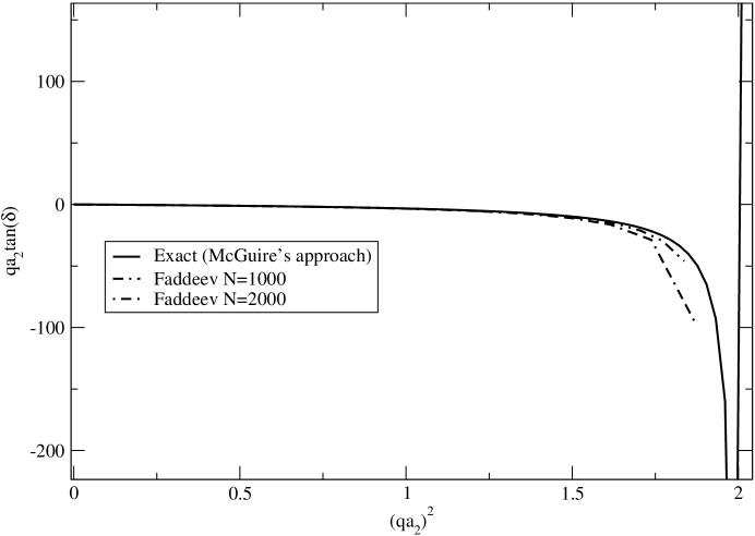
Figure 1: The effective range expansion found by numerical solution to the Faddeev equation is shown.

IV Adiabatic Curves and the Eigenchannel R-Matrix Solution

The final apprach involves the adiabatic representation and the eigenchannel R-matrix method. We refer the interested reader to appendix A for a review of these tools. For $\delta$-function interactions, the eigenstates of the adiabatic Hamiltonian inside one of the six regions are simply solutions to the free Schrödinger equation. As long as we restrict our analysis to one of the six regions, the solution may be found by separation of variables and must be of the form Gibson et al. (1987)

$$\phi_{0}(\rho,\theta)=A_{0}(\rho)\cosh{(q_{0}\theta)}$$ (20)

$$\phi_{n}(\rho,\theta)=A_{n}(\rho)\cos{(q_{n}\theta)}$$ (21)

We must treat $\phi_{0}$ as a special case since it represents the only channel with a two-body bound state. The eigenvalue is found by demanding continuity of the wavefunction at the $\delta$-function surface. If we restrict our analysis to the region $\theta\in(0,\pi/3)$, then integration of the Schrödinger equation from $\pi/6-\epsilon$ to $\pi/6+\epsilon$ leads to the following transcendental equations for $q_{n}$

$$q_{0}\tanh{(\frac{q_{0}\pi}{6})}=\frac{\sqrt{2}\rho}{a_{2}}$$ (22)

$$q_{n}\tan{(\frac{q_{n}\pi}{6})}=-\frac{\sqrt{2}\rho}{a_{2}}$$ (23)

Normalization of $\phi_{n}$ gives:

$$A_{0}(\rho)=\left[\pi+\frac{3}{q_{0}}\sinh{\left(\frac{q_{0}\rho\pi}{3}\right)}\right]^{-\frac{1}{2}}$$ (24)

$$A_{n}(\rho)=\left[\pi+\frac{3}{q_{n}}\sin{\left(\frac{q_{0}\rho\pi}{3}\right)}\right]^{-\frac{1}{2}}$$ (25)

The adiabatic potential $U_{n}$ is related to $q_{n}$ by:

$$U_{0}(\rho)=\frac{-q_{0}^{2}}{2m\rho^{2}}$$ (26)

$$U_{n}(\rho)=\frac{q_{n}^{2}}{2m\rho^{2}}$$ (27)

We’ve verified that our potential curves are in agreement with those presented in Gibson et al. (1987). We provide a plot of the first few in Fig. 2. As expected, there is only one attractive channel which is open below the dimer (two-body bound state) breakup threshold.

Figure 2: The adiabatic potential curves for the $\delta$-function interaction are shown.

This model supports one true bound state with energy $E=-4B_{2}$. We’ve found that a calculation with one adiabatic channel under-binds this state by about $0.03B_{2}$. Further, the inclusion of more coupled adiabatic channels does not serve to improve our result. A calculation without the diagonal coupling term gives a second bound state at $-1.00213B_{2}$, very close to threshold. When the repulsive diagonal coupling is included, this bound state is no longer supported and its eigenenergy is above the two-body binding. The presence of such a state is of course consistent with the fact that the exact scattering solution indicates a divergent scattering length. A table of these results is shown in Table 2.

Table 2: Eigenenergies for the $\delta$-function model using the adiabatic representation. All energies are in units of the two-body binding $B_{2}$.

Level	Exact	1 channel no $Q_{00}$	1 channel with $Q_{00}$	5 channels full calculation	Faddeev
1	-4	-3.96902	-3.96106	-3.96106	-3.9998
2	-1	-1.00213	-0.99587	-0.99587	-1.0000

For the case in question, the matrix elements in Eq. 67 and Eq. 68 take the form (compare with Eq. (57)):

$$\Lambda_{m,n}=\rho_{0}F_{m}(\rho_{0})F_{n}(\rho_{0})$$ (28)

$$\Gamma_{m,n} =\int_{0}^{\rho_{0}}{\rho d\rho\hskip 3.61371pt\delta_{m,n}\left[-\frac{\partial F_{m}}{\partial\rho}\frac{\partial F_{n}}{\partial\rho}+F_{m}F_{n}(k^{2}-2mU_{n}(\rho))\right]}$$

$$+\int_{0}^{\rho_{0}}{\rho d\rho\left[P_{m,n}(\rho)F_{m}\left(2\frac{\partial}{\partial\rho}+\frac{1}{\rho}\right)F_{n}+Q_{m,n}F_{m}F_{n}\right]}$$ (29)

We choose a set of $7^{\text{th}}$ order b-splines as our basis set in the expansion for the the functions $F_{n}(\rho)$. Basis splines have proven to be a versatile and efficient basis set for a wide variety systems van der hart (1997); Johnson et al. (1988); Bortolotti and Bohn (2004). See de Boor (1978) for mathematical details, fast algorithms and fortran code. The results presented in Fig. 3 and Table 2 are for a set of $40$ splines with a quadratic distribution of knot points over the region $\rho\in[0,20\>a_{2}]$.

In the scattering sector, there are a number of subtleties involved with the matching of the wavefunction in the asymptotic region. If the diagonal coupling term is ignored, then the Schrödinger equation in the ground state channel for $\rho\rightarrow\infty$ takes the form:

$$\left[-\frac{\partial^{2}}{\partial\rho^{2}}-\frac{1}{\rho}\frac{\partial^{2}}{\partial\rho^{2}}+k_{0}^{2}-k^{2}\right]F_{0}(\rho)=0$$ (30)

This is recognized as the zeroth order Bessel’s equation, and hence $f$ must be of the form:

$$F_{0}(\rho)=AJ_{0}(q\rho)+BY_{0}(q\rho)$$ (31)

where $q^{2}=k^{2}-k_{0}^{2}$. If the diagonal coupling is included, then the solution must satisfy

$$\left[-\frac{\partial^{2}}{\partial\rho^{2}}-\frac{1}{\rho}\frac{\partial^{2}}{\partial\rho^{2}}+k_{0}^{2}-k^{2}-Q_{00}(\rho)\right]F_{0}(\rho)=0.$$ (32)

$Q_{00}$ behaves asymptotically as $1/4\rho^{2}$, meaning that the solutions must now be fractional order Bessel functions,

$$F_{0}(\rho)=AJ_{1/2}(q\rho)+BY_{1/2}(q\rho).$$ (33)

Reference Amaya-Tapia et al. (1997) defines the scattering matrix in terms of the outgoing wavefunction as

$$F_{0}(\rho)\rightarrow\sqrt{(q\rho)}(H^{(2)}_{1/2}(q\rho)+e^{2i\delta^{\prime}}H^{(1)}_{1/2}(q\rho)),$$ (34)

which, ignoring overall normalization, and taking $q\rho\gg 1$, can be written

$$.F_{0}(\rho)\rightarrow e^{-iq\rho}-e^{2i\delta^{\prime}}e^{iq\rho}$$ (35)

Reference Amaya-Tapia et al. (1997) asserts that the minus sign appearing above adds an extra $\pi/2$ to the phase-shift, so that the total phase shift starts at $3\pi/2$. This assertion would indeed be consistent with Levinson’s theorem in three-dimensions, where one would obtain a $\pi$ from the known bound state and a $\pi/2$ from the zero-energy resonance. However, in one spatial dimension, we note that there is no additional $\pi/2$ for the zero-energy resonance. The statement of Levinson’s theorem in one dimension for the even parity solution takes the form de Bianchi (1994); Gibson (1987)

$$\lim_{k\rightarrow 0}\delta_{e} =(n_{e}-1/2)\pi$$ noncritical case (36)

$$\lim_{k\rightarrow 0}\delta_{e} =n_{e}\pi \text{critical case}.$$ (37)

The critical case applies when there is a zero-energy resonance. The statement for the odd-parity solution is identical to that for three-dimensional S-waves:

$$\lim_{k\rightarrow 0}\delta_{o} =n_{o}\pi$$ noncritical case (38)

$$\lim_{k\rightarrow 0}\delta_{o} =(n_{o}+1/2)\pi$$ critical case (39)

We are concerned only with the even parity case. We define our scattering matrix in the following fashion. We require $S$ to be the coefficient multiplying the outgoing $e^{iq\rho}$ in the limit $q\rho\gg 1$. In terms of the out-going wavefunction, this means

$$F_{0}(\rho)\rightarrow\frac{1}{\sqrt{q\rho}}(e^{-iq\rho}+e^{2i\delta}e^{iq\rho}).$$ (40)

We justify our choice by considering the limit $\xi_{1}\ll\xi_{2}$, which is appropriate when particles 1 and 2 are bound and particle 3 is far away, in which case, $\rho\approx\xi_{2}(1+\frac{1}{2}\frac{\xi 1^{2}}{\xi_{2}^{2}}...)$. In this way, the product $F_{0}(\rho)\phi_{0}(\rho,\theta)$ represents a 2-particle bound state in one relative coordinate and an oscillatory wave in the second relative coordinate, symeterized over all permutations of particles. Note also that the extra factor of $1/\sqrt{q\rho}$ appearing in our asymptotic solution is different from the convention of reference Amaya-Tapia et al. (1997); this is because we choose to work with the full wavefunction instead of the reduced wavefunction, hence our integration measure remains $\int{\rho\>d\rho\>d\theta}$.

In terms of standing wave solutions, the definition of the phase-shift above is consistent with the following expression involving $\tan{(\delta)}$:

$$F_{0}(\rho)\rightarrow\frac{1}{\sqrt{q\rho}}(\cos{(q\rho)}-\tan{(\delta)}\sin{q\rho})$$ (41)

The form in Eq. (41) leads to the desired product state corresponding to 1+2 scattering in one dimension. By identifying

$$b=-\frac{\partial\ln{F_{0}(\rho)}}{\partial\rho},$$ (42)

one may easily solve for $\tan{\delta}$. An alternative argument may be formulated by simply noting that the normalization condition $\int{\frac{d\theta}{2\pi}\phi_{0}^{2}(\rho,\theta)}=1$ requires that $\phi_{0}$ scale like $\sqrt{\rho}$. This means that the full wavefunction is proportional to the quantity $\sqrt{\rho}F_{0}(\rho)$. If we consider the wavefunction at a particular angle, and let $\Psi(\rho,\theta=\theta_{0})\rightarrow A\cos{(q\rho+\delta)}$, which is the proper asymptotic form for an even solution, then

$$\frac{\partial\ln{\Psi(\rho,\theta=\theta_{0})}}{\partial\rho}=-b+\frac{1}{2\rho}=-q\tan{(q\rho+\delta)}.$$ (43)

This expression is entirely equivalent to the matching condition Eq. 42. We note that our phase shift $\delta$ is related to $\delta^{\prime}$ by

$$\tan{\delta}=\frac{-1}{\tan{\delta^{\prime}}}$$ (44)

Clearly, this will alter the behavior at threshold. We note that with our definition, the presence of a zero energy resonance is consistent with the threshold behavior of the effective range expansion, namely that the 1+2 scattering length is divergent.

Figure 3: The effective range expansion for 1+2 scattering with $\delta$=function interactions calculated using the Eigenchannel R-Matrix method is shown. A calculation with five coupled channels is well converged such that the inclusion of more channels does alter the results.

V Discussion

The most striking feature of these results is the presence of the zero-energy resonance marked by the divergent scattering length. As the cutoff is lowered and the range of the interaction becomes finite, the scattering amplitude in the limit $k\rightarrow 0$ becomes nonzero. This behavior is illustrated in the off-shell amplitude calculated numerically via Eq. 91 (except with a principal value prescription) shown in Fig. 4, which is the 1D analog of Fig. 5 appearing in reference Bedaque et al. (1999). There is clearly a fixed point in the limit $\Lambda\rightarrow\infty$. The presence of the zero-energy resonance is further substantiated by the variational calculations of Section IV. When the repulsive second-derivative coupling $Q_{0,0}(\rho)$ is omitted, the interaction supports a second bound state with energy $E=-1.00213B_{2}$. When $Q_{0,0}(\rho)$ is included, the bound state is no longer supported and a solution to Eq. 56 gives $E>-B_{2}$, consistent with the upper bound theorem. These results are also consistent with the threshold behaviour of $qa_{2}\tan{\delta}$ shown in Fig. 6. The Eigenchannel R-Matrix method gives $\lim_{qa_{2}\rightarrow 0}{qa_{2}\tan{\delta}}\approx 0.065$ when the diagonal coupling is excluded, and $\lim_{qa_{2}\rightarrow 0}{qa_{2}\tan{\delta}}\approx-0.008$ when it is included. Finally, the exact effective range expansion calculated in Section II indicates a divergent scattering length in perfect agreement with the numerical calculations. It is again of considerable note that the zero energy resonance is present regardless of the value of the $\delta$-function coupling, or equivalently the two-body scattering length. It appears at exactly zero relative energy in the 1+2 system as long as the two-body interactions are of zero range, and moves away from threshold as the interactions become of finite range.

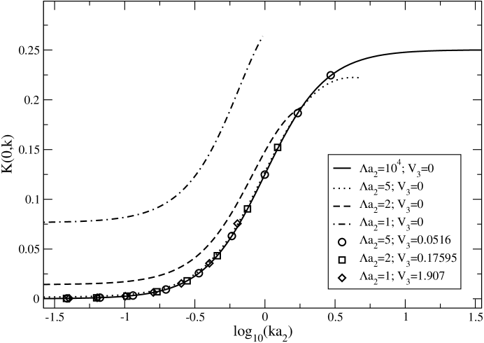
Figure 4: The off-shell amplitude for our one dimensional model is shown. The black curve which should be considered the “exact” result is for $\Lambda a_{2}=10^{4}$. As the cutoff is lowered to $\Lambda a_{2}=5$, a three-body term with $V_{3}=-0.0516$ brings $K(0,0)$ into agreement with the exact result. As the cutoff is lowered further to $\Lambda a_{2}=2$, a three-body term with $V_{3}=-0.17595$ is required. Finally, $V_{3}=-1.907$ produces the exact $K(0,0)$ for $\Lambda a_{2}=1$.

Figure 5: The on-shell amplitude for our one dimensional model is shown for various values of the cutoff. As the cutoff is lowered, a three-body contact interaction of natural size is introduced to fix the 1+2 scattering length.

.

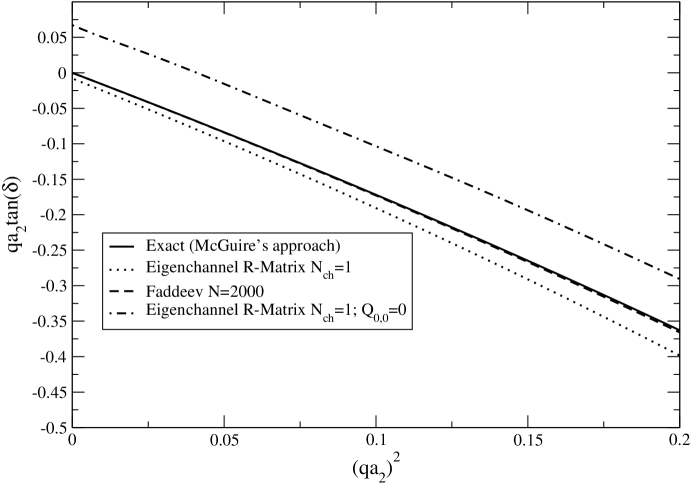
Figure 6: The effective range expansion near the region $qa_{2}\rightarrow 0$ is shown for various calculations.

It is now instructive to consider the on-shell results when various cutoffs are enforced in Eq. 91. As the cutoff is lowered, we require that $1/a_{3}=0$ ($a_{3}$ being the 1+2 scattering length). This quantity is proportional to the scattering amplitude satisfied by the principal value version of Eq. 91. With the introduction of a three-body interaction, the cutoff dependence of the amplitude can be absorbed into the three-body coupling $V_{3}$, yielding a largely cutoff invariant amplitude as seen if Fig. 4 and Fig. 5.

This paper has treated three bosons only at zeroth order in EFT. In a second paper, we shall extend the analysis to include the two-body effective range and shape parameter. Predictions from the resulting EFT will be compared to calculations using a realistic phenomenological NN interaction. Three-nucleon observables will serve as a testing ground for the effective theory.

Appendix A Review of the Adiabatic Hyperspherical Representation and the Eigenchannel R-Matrix method

The essential strategy for solving the Schrödinger equation in coordinate space is to transform the partial differential equation (PDE) into a set of coupled ordinary differential equations (ODEs). While there are a variety of representations that realize this goal, the one best suited to the present problem is the adiabatic hyperspherical representation Macek (1968) (see also Fano (1981)).

Let us first introduce the appropriate relative and hyperspherical coordinates. Jacobi coordinates in one dimension for equal masses are defined via

$$\left(\begin{array}[]{c}X\\ \xi_{1}\\ \xi_{2}\end{array}\right)=\left(\begin{array}[]{ccc}\frac{1}{\sqrt{3}}&\frac{1}{\sqrt{3}}&\frac{1}{\sqrt{3}}\\ \frac{1}{\sqrt{2}}&\frac{-1}{\sqrt{2}}&0\\ \frac{1}{\sqrt{6}}&\frac{1}{\sqrt{6}}&\frac{-2}{\sqrt{6}}\end{array}\right)\left(\begin{array}[]{c}x_{1}\\ x_{2}\\ x_{3}\end{array}\right)$$ (45)

where $X$ marks the position of the total center-of-mass, $\xi_{1}$ is the relative coordinate for the first two particles , and $\xi_{2}$ is the relative coordinate between third particle to the center-of-mass of the first two. Hyperspherical coordinates in one dimension are simply circular polar coordinates:

$$\xi_{1} =\rho\cos{\theta}$$ (46)

$$\xi_{2} =\rho\sin{\theta}$$ (47)

$$\rho^{2} =\xi_{1}^{2}+\xi_{2}^{2}$$ (48)

Here, $\rho$ is a measure of the general size of the system. At small values of $\rho$, all three particles are in close proximity, while at large values of $\rho$, the situation depends on the angle $\theta$. There are some values of $\theta$ that correspond to two of the three particles being near each other, and other values of $\theta$ where all three particles are far apart.

With this transformation, the Schrödinger equation becomes (compare with Eq. 1)

$$\left\{\frac{1}{\rho}\frac{\partial}{\partial\rho}\left(\rho\frac{\partial}{\partial\rho}\right)+\frac{1}{\rho^{2}}\frac{\partial^{2}}{\partial\theta^{2}}+k^{2}-U(\rho,\theta)\right\}\Psi(\rho,\theta)=0$$ (49)

where $k^{2}=2mE$ and

$$U(\rho,\theta)=2m\Big{(} V(\sqrt{2}\rho|\cos(\theta)|)+$$

$$V(\sqrt{2}\rho|\cos(\theta+\pi/3)|)+V(\sqrt{2}\rho|\cos(\theta-\pi/3)|)\Big{)}.$$ (50)

This potential has a very high degree of symmetry:

$$U(\rho,\theta) =U(\rho,\theta\pm\frac{\pi}{3})\hskip 72.26999pt$$ exchange (51)

$$U(\rho,\theta) =U(\rho,-\theta)$$ parity (52)

The combination of exchange and parity result in a six-fold symmetry allowing the angular part of the wavefunction to be represented as a sum over terms proportional to $\cos{6n\theta}$.

The reduction of the PDE Eq. 49 into a set of coupled ODEs is accomplished by expanding the wave function into a sum over different adiabatic channels:

$$\Psi(\rho,\theta)=\sum_{n}\psi_{n}(\rho,\theta)=\sum_{n}{\phi_{n}(\rho,\theta)F_{n}(\rho)}.$$ (53)

where $\phi_{n}$ are defined as eigenstates of the adiabatic Hamiltonian:

$$H_{ad}(\rho,\theta)\phi_{n}(\rho,\theta)=k_{n}^{2}(\rho)\phi_{n}(\rho,\theta)$$ (54)

with

$$H_{ad}(\rho,\theta)=\frac{-1}{\rho^{2}}\frac{\partial^{2}}{\partial\theta^{2}}+U(\rho,\theta).$$ (55)

It is important to note that Eq. 54 depends only parametrically on $\rho$. We impose boundary conditions such that $\phi_{n}$ is even at $\theta=0$ and $\theta=\pi/6$. Inserting the expansion in Eq. (53) into a variational expression of the form

$$k^{2}=\frac{\int_{V}{dV\>\Psi^{\dagger}(-\nabla^{2}+U)\Psi}}{\int_{V}{dV\>\Psi^{\dagger}\Psi}}$$ (56)

and demanding that the solution be stationary with respect to variations in the functions $F_{m}^{\dagger}$, one arrives at the following matrix equation:

$$(\mathbf{T}+\mathbf{U})\mathbf{F}=k^{2}\mathbf{F}.$$ (57)

We’ve defined

$$T_{m,n}=-\delta_{m,n}\left(\frac{\partial^{2}}{\partial\rho^{2}}+\frac{2}{\rho}\frac{\partial}{\partial\rho}\right)-P_{m,n}(\rho)\left(2\frac{\partial}{\partial\rho}+\frac{2}{\rho}\right)-Q_{m,n}(\rho)$$ (58)

and

$$U_{m,n}(\rho)=\delta_{m,n}(k^{2}_{m}(\rho)).$$ (59)

Also, we’ve introduced the non-adiabatic channel couplings defined as

$$P_{m,n}(\rho)=\Big{\langle}\phi_{m}\Big{|}\frac{\partial}{\partial\rho}\phi_{n}\Big{\rangle},$$ (60)

$$Q_{m,n}(\rho)=\Big{\langle}\phi_{m}\Big{|}\frac{\partial^{2}}{\partial\rho^{2}}\phi_{n}\Big{\rangle}.$$ (61)

The solution of the the adiabatic equatation Eq. 54. Eq. (55) and the evaluation of the first and second derivative couplings accounts for the vast majority of the computational effort in solving the three-body problem using this approach. The first-derivative couplings $P_{m,n}$ can be evaluated using a Feynman-Hellman like argument. For a $\rho$-parameterized system defined by $H(\rho)\phi=E(\rho)\phi$, the Feynman-Hellman theorem states

$$\frac{dE}{d\rho}=\Big{\langle}\phi\Big{|}\frac{\partial H}{\partial\rho}\Big{|}\phi\Big{\rangle}.$$ (62)

This relation can be used to find that

$$\Big{\langle}\phi_{m}\Big{|}\frac{\partial}{\partial\rho}{\phi_{n}}\Big{\rangle}=\frac{\langle\phi_{m}\Big{|}\frac{\partial H}{\partial\rho}\Big{|}\phi_{n}\rangle}{k^{2}_{n}(\rho)-k^{2}_{m}(\rho)}$$ (63)

for $m\neq n$, and vanishes for m=n. The second-derivative couplings, $Q_{m,n}$, may be readily calculated by noting:

$$Q_{m,n}=[P^{2}]_{m,n}+\left[\frac{\partial P}{\partial\rho}\right]_{m,n}.$$ (64)

Use of the above relation, however requires calculating the first-derivative couplings between many channels so that the square of $P$ converges. For calculations involving a single adiabatic channel, it is more convenient to estimate $Q_{0,0}$ by using a 3-point or 5-point rule. This involves solving the adiabatic Hamiltonian at three consecutive nearby values of the parameter $\rho$, and calculating the second derivative numerically before evaluating the inner product.

In order to calculate wavefunctions and scattering amplitudes in the scattering sector, we use the Eigenchannel R-matrix approach Greene (1983); Aymar et al. (1996), which is a variational calculation for minus the log-derivative of the wave function on the surface $S$ of some reaction volume $V$. More precisely, this method finds variational solutions that have a constant log-derivative on the surface such that $\frac{\partial\Psi}{\partial n}+b\Psi=0$.

Starting with Eq. 56, we define $b=-\frac{\partial{ln(\Psi)}}{\partial{\hat{n}}}$, where $\hat{n}$ represents the unit normal vector to the reaction surface $S$ ($\hat{n}=\hat{\rho}$ in our case); application of Green’s theorem to the kinetic energy term in Eq. (56) allows us to write an expression for $b$ at a fixed $k^{2}$.

$$b=\frac{\int_{V}{dV\left[(-\vec{\nabla\Psi^{\dagger}}\cdot\vec{\nabla\Psi})+\Psi^{\dagger}(k^{2}-U)\Psi\right]}}{\int_{S}{dS\>\Psi^{\dagger}\Psi}}$$ (65)

Note that we were able to factor $b$ out of the surface integral in the denominator only because the desired solution has a constant log-derivative on the surface $S$. Eq. (65) is an identity obeyed by exact eigenstates of the Schrödinger equation Eq. (49) that have a constant $b$ on $S$. By taking the first-order variation of this expression with respect to small deviations in $\Psi$, this expression can be shown to be a variational expression for $b$.

In the adiabatic representation, we expanded the wavefunction according to Eq. 53. Now we expand $F_{n}=\sum_{\alpha}{c_{n,\alpha}B_{\alpha}}$, and Eq. (65) is cast into the form of a generalized eigenvalue equation:

$$b\mathbf{\Lambda}\mathbf{c}=\mathbf{\Gamma}\mathbf{c}\hskip 72.26999ptb=-\frac{\partial\ln{\Psi(\rho)}}{\partial\rho}$$ (66)

where

$$\Lambda_{m,n}=\int_{S}{\vec{dS}\cdot\hat{n}\;\psi_{m}\psi_{n}}$$ (67)

$$\Gamma_{m,n}=\int_{V}{dV[-\vec{\nabla\psi_{m}}\cdot\vec{\nabla\psi_{n}}+\psi_{m}(k^{2}-U)\psi_{n}]}$$ (68)

Appendix B Derivation of Faddeev Equations

In this section, we derive the properly symeterized integral equation satisfied by the scattering amplitude for one free boson off of a bound pair. Our derivation relies heavily on the original work of Faddeev Faddeev (1965), Lovelace Lovlace (1964) and Amado Amado (1963), however we largely hold to the notation conventions of Watson and Nuttall Watson et al. (1967). We shall begin by calculating the two-boy scattering amplitude for a separable interaction of the form:

$$V=c_{0}|g\rangle\langle g|,$$ (69)

with momentum space matrix elements:

$$\langle q^{\prime}|V|q\rangle=c_{0}g(q^{\prime})g(q).$$ (70)

The $T$-matrix element $\langle q^{\prime}|T(E)|q\rangle$ satisfies the Lippman-Schwinger equation:

$$T(q^{\prime},q,E)=c_{0}g(q^{\prime})g(q)+c_{0}g(q^{\prime})\int{\frac{dq^{\prime\prime}}{2\pi}\frac{mg(q^{\prime\prime})T(q^{\prime\prime},q,E)}{mE-q^{\prime\prime 2}}}$$ (71)

The solution is found by defining the energy dependent function Watson et al. (1967)

$$h(q,E)=\int{\frac{dq^{\prime\prime}}{2\pi}\frac{mg(q^{\prime\prime})T(q^{\prime\prime},q,E)}{mE-q^{\prime\prime 2}}}$$ (72)

which satisfies the algebraic equation:

$$h(q,E)=\left[\int{\frac{dq^{\prime\prime}}{2\pi}\frac{mg^{2}(q^{\prime\prime})}{mE-q^{\prime\prime 2}}}\right][c_{0}g(q)+c_{0}h(q,E)].$$ (73)

Solving for $h(q,E)$ and substituting the result into the Lippman-Schwinger equation quickly yields the solution:

$$T(q^{\prime},q,E)=g(q^{\prime})g(q)\left[\frac{1}{c_{0}}-\int{\frac{dq^{\prime\prime}}{2\pi}\frac{mg^{2}(q^{\prime\prime})}{mE-q^{\prime\prime 2}}}\right]^{-1}$$ (74)

Taking the limit $g(q)\rightarrow 1$ is equivalent to solving the corresponding Schrödinger equation with contact interactions. This yields a $T$-matrix element independent of $q$ and $q^{\prime}$:

$$mT(E+i\epsilon)=mc_{0}\left[1+\frac{mc_{0}}{2\sqrt{-mE-i\epsilon}}\right]^{-1}.$$ (75)

In the center of mass frame, the energy is written $E=k^{2}/m$ and the scattering amplitude $f$ for the even parity wave is related to the on-shell $T$-matrix by:

$$f=\frac{1}{2}\left(e^{2i\delta}-1\right)=\frac{i\tan\delta}{1-i\tan\delta}=\frac{mT(k,k,E)}{2ik}=\frac{\frac{mc_{0}}{2ik}}{1-\frac{mc_{0}}{2ik}}.$$ (76)

The cross-section is a normalized probability in one dimension and is given by $\sigma=|f|^{2}$.

If the coupling is negative, the interaction supports a bound state. The $T$-matrix element will exhibit a pole at the binding energy $E=-B_{2}$. From inspection of Eq. (75), it is clear that this requires $B_{2}=mc_{0}^{2}/4=1/ma_{2}^{2}$. The state vector for the bound state is:

$$|\psi_{B}\rangle=\sqrt{N}G_{0}(-B_{2})|g\rangle.$$ (77)

where $G_{0}(-B_{2})=(-B_{2}-H_{0})^{-1}$ is the free particle propagator evaluated at the bound state energy. The normalization constant is easily evaluated by contour integration to be

$$N^{-1}=\langle g|G_{0}^{2}(-B_{2})|g\rangle=\frac{m^{2}a_{2}^{3}}{4}.$$ (78)

The indices in the three-body sector follow the convenient “odd-man-out” notation. When considering matrix elements of two-body operators in the three-body state-space, the two-body operator $V_{\alpha}$ with $\alpha=1$ shall denote the interaction between particles $2$ and $3$. We are only concerned with internal degrees of freedom, and will therefore work in the total center of momentum frame $p_{1}+p_{2}+p_{3}=0$. Matrix elements will be taken with respect to state vectors of the form $|p_{\alpha},q_{\alpha}\rangle$, where $p_{\alpha}$ represents the momentum of the spectator particle $\alpha$, and $q_{\alpha}$ represents the relative momentum of the remaining two particles. Let $|\psi_{\alpha}^{+}\rangle=|\psi_{\alpha}^{(1)}\rangle+|\psi_{\alpha}^{(2)}\rangle+|\psi_{\alpha}^{(3)}\rangle$ describe an eigenstate of the full Hamiltonian $H$ which corresponds to an initial state $|\chi_{\alpha}\rangle$ with the two particles not equal to $\alpha$ forming a bound state. The solution is found by solving the Faddeev equations for the components $|\psi_{\alpha}^{(\beta)}\rangle$:

$$|\psi_{\alpha}^{(\beta)}\rangle=G_{0}(E)|\alpha,p_{\alpha}\rangle\delta_{\alpha\beta}+\sum_{\gamma\neq\beta}{G_{0}(E)T_{\beta}|\psi_{\alpha}^{(\gamma)}\rangle}.$$ (79)

We write the two-body T-matrix in the three-body state space as:

$$T_{\beta}(E)=\int{\frac{dp_{\beta}}{2\pi}|\beta,p_{\beta}\rangle\tau_{\beta}\left(E-\frac{3p_{\beta}^{2}}{4m}\right)\langle\beta,p_{\beta}|}$$ (80)

where $\tau_{\beta}(E)$ is the dimer propagator in the $\beta$ channel:

$$\tau_{\beta}(E)=\left[\frac{1}{c_{0}}+\int{\frac{dq}{2\pi}\frac{mg_{\beta}^{2}(q)}{q^{2}-mE}}\right]^{-1}$$ (81)

For $g_{\beta}(q)\rightarrow 1$, $\tau_{\beta}(E)$ is equal to the two-body T-matrix found in the previous section. left multiplying Eq. (79) by $\langle\delta,p_{\delta}|$ and summing over $\beta\neq\delta$ leads to:

$$X_{\delta,\alpha}(p_{\delta},p_{\alpha})=Z_{\delta,\alpha}(p_{\delta},p_{\alpha})+\sum_{\beta}{\int{\frac{dp_{\beta}}{2\pi}Z_{\delta,\beta}(p_{\delta},p_{\beta})\tau_{\beta}\left(E-\frac{3p_{\beta}^{2}}{4m}\right)X_{\beta,\alpha}(p_{\beta},p_{\alpha})}}.$$ (82)

The amplitudes $X_{\delta,\alpha}(p_{\delta},p_{\alpha})$ and $Z_{\delta,\alpha}(p_{\delta},p_{\alpha})$ are defined as:

$$X_{\delta,\alpha}(p_{\delta},p_{\alpha}) =\sum_{\gamma\neq\delta}{\langle\delta,p_{\delta}|\psi_{\alpha}^{(\gamma)}\rangle.}$$ (83)

$$Z_{\delta,\alpha}(p_{\delta},p_{\alpha}) =(1-\delta_{\delta\alpha})\langle\delta,p_{\delta}|G_{0}(E)|\alpha,p_{\alpha}\rangle.$$ (84)

The Born amplitude $Z_{\delta,\alpha}(p_{\delta},p_{\alpha})$ describes the interaction mediated by the exchange of a single particle, and requires calculating $q_{\delta}$ in terms of $p_{\alpha}$ with $\delta\neq\alpha$. The kinematics for a given case must be determined by cyclic permutation of the particles Lovlace (1964). For example,

$$Z_{2,1}(p_{2},p_{1})=\frac{g_{2}\left(-p_{1}-\frac{1}{2}p_{2}\right)g_{1}\left(p_{2}+\frac{1}{2}p_{1}\right)}{E-\frac{3p_{1}^{2}}{4m}-\frac{1}{m}\left(p_{2}+\frac{1}{2}p_{1}\right)^{2}}.$$ (85)

For identical bosons the quantity of interest is the symeterized amplitude given by the sum of the direct and exchange pieces $X(p,k;E)=X^{(D)}(p,k;E)+2X^{(N)}(p,k;E)$. This amplitude satisfies the following integral equation:

$$X(p,k;E)=2Z(p,k;E)+2\int{\frac{dq}{2\pi}Z(p,q;E)\tau\left(E-\frac{3q^{2}}{4m}\right)X(q,k;E)}$$ (86)

where the Born term for $g(q)\rightarrow 1$ is given by:

$$Z(p,q;E)=\frac{m}{mE-q^{2}-p^{2}-q\cdot p},$$ (87)

and the total energy is $E=\frac{3k^{2}}{4m}-B_{2}$. Next we perform an angle average over the dot product. In one dimension the angle average of an arbitrary function $f(p\cdot q)$ is $\bar{f}=\frac{1}{2}(f(pq)+f(-pq))$, and so the Born amplitude becomes:

$$Z(p,q;E)=\frac{mE-q^{2}-p^{2}}{(mE-q^{2}-p^{2})^{2}-p^{2}q^{2}}.$$ (88)

The desired amplitude now satisfies the integral equation:

$$\frac{X(p,k,E+i\epsilon)}{2m} =Z(p,k,E)$$

$$\>+4\int{\frac{dq}{2\pi}Z(p,q,E)\left[-a_{2}+\frac{1}{\sqrt{-mE+\frac{3q^{2}}{4}-i\epsilon}}\right]^{-1}\frac{X(q,k,E+i\epsilon)}{2m}}.$$ (89)

It is desirable to remove the pole in the dimer propagator and bring this equation into the form of the Lippman-Schwinger equation; to this end we define the amplitude:

$$\frac{\tilde{X}(p,k,E)}{k^{2}-p^{2}}=\left[-a_{2}+\frac{1}{\sqrt{-mE+\frac{3p^{2}}{4}}}\right]^{-1}\frac{X(p,k,E)}{2m}$$ (90)

A bit of algebra shows that the new amplitude satisfies the equation:

$$\tilde{X}(p,k,E+i\epsilon)=\tilde{Z}(p,k,E+i\epsilon)-\frac{4}{\pi}\int_{0}^{\infty}{dq\>\tilde{Z}(q,p,E+i\epsilon)\frac{\tilde{X}(q,k,E+i\epsilon)}{q^{2}-k^{2}-i\epsilon}}$$ (91)

with

$$\tilde{Z}(q,p,E)=\left[\frac{mE-q^{2}-p^{2}}{(mE-q^{2}-p^{2})-p^{2}q^{2}}\right]\frac{4}{3a_{2}^{2}}\sqrt{-mE+\frac{3p^{2}}{4}}\left[1+a_{2}\sqrt{-mE+\frac{3p^{2}}{4}}\right].$$ (92)

It is computationally more convenient to deal with an amplitude which is real below the breakup threshold by writing the above integral equation in terms of a principal value prescription using the well known formula:

$$\frac{1}{\omega\pm i\epsilon}=\mathcal{P}\mp i\pi\delta(\omega)$$ (93)

Appendix C Alternative derivation of Eq. 86

Bedaque et al Bedaque et al. (1999) have considered the 3-D three-body problem with short range interactions in a ground-breaking paper. It is instructive to consider their approach in a 1-D context, and that is the purpose of this appendix; a complete analytic sum of the series arising in perturbation theory has been found by Thacker Thacker (1974).

Consider the Feynman rules resulting from the Lagrangian density:

$$\mathcal{L}=\phi^{\dagger}(x)\left(i\partial_{0}+\frac{\partial_{x}^{2}}{2m}\right)\phi(x)-\frac{c_{0}}{2}\left(\phi^{\dagger}(x)\phi(x)\right)^{2}-\frac{d_{0}}{6}\left(\phi^{\dagger}(x)\phi(x)\right)^{3}.$$ (94)

Let us first sum the perturbative series of bubble diagrams for the two-body problem with $d_{0}=0$. Let $(p_{0},\vec{p})=(\frac{1}{4m}(k_{1}-k_{2})^{2},k_{1}+k_{2})$ with $|k_{1}|=k$ denote the two-vector in the center of momentum frame. The following loop integral is readily evaluated by contour integration:

$$L =\int{\frac{d\vec{q}}{2\pi}\frac{dq_{0}}{2\pi}\frac{i}{\frac{p_{0}}{2}-q_{0}-\frac{1}{2m}(\frac{\vec{p}}{2}-\vec{q})^{2}+i\epsilon}\frac{i}{\frac{p_{0}}{2}+q_{0}-\frac{1}{2m}(\frac{\vec{p}}{2}+\vec{q})^{2}+i\epsilon}}$$ (95)

$$=\frac{-im}{2\sqrt{-mp_{0}+\frac{\vec{p}^{2}}{4}-i\epsilon}}=\frac{m}{2k},$$ (96)

and the geometric series is easily summed to reproduce the result of Section B:

$$iA=-iT=-ic_{0}\left(1+(-ic_{0}L)+(-ic_{0}L)^{2}...\right)=\frac{-ic_{0}}{1+ic_{0}L}=\frac{-ic_{0}}{1-\frac{mc_{0}}{2ik}}.$$ (97)

Kaplan Kaplan (1997) suggested that the Lagrangian Eq. 94 may be conveniently rewritten in terms of a dummy field $D$:

$$\mathcal{L}=\phi^{\dagger}\left(i\partial_{0}+\frac{\partial_{x}^{2}}{2m}\right)\phi+\Delta D^{\dagger}D-\frac{g}{\sqrt{2}}(D^{\dagger}\phi\phi+\phi^{\dagger}\phi^{\dagger}D)+h(D^{\dagger}D\phi^{\dagger}\phi+\phi\phi^{\dagger}DD^{\dagger})$$ (98)

Gaussian path integration over the auxiliary field $D$ shows that the couplings appearing in Eq. (98) are related to those in Eq. (94) by $g^{2}/\Delta=c_{0}$ and $-3hg^{2}/\Delta^{2}=d_{0}$. The bare dimer propagator is $i/\Delta$, while the sum of diagrams shown in Fig. 7 yields

$$i\Delta(p_{0},\vec{p}) =\frac{i}{\Delta}\left(1+\left(\frac{-ig^{2}L}{\Delta}\right)+\left(\frac{-ig^{2}L}{\Delta}\right)^{2}+\>...\right)$$ (99)

$$=\frac{i}{\Delta+\frac{mg^{2}}{2}(-mp_{0}+\frac{\vec{p}^{2}}{4}-i\epsilon)^{-1/2}}.$$ (100)

Figure 7: The dressed dimer propagator determined by the geometric series of loop insertions.

For the 1+2 integral equation, we choose the same kinematics as Bedaque et al Bedaque et al. (1999). Let the incoming particle and dimer have two-momenta $(k^{2}/2m,-\vec{k})$ and $(k^{2}/4m-B_{2},\vec{k})$, respectively. The outgoing particle and dimer are off-shell with two-momenta $(k^{2}/2m-\varepsilon,-\vec{p})$ and $(k^{2}/4m-B_{2}+\varepsilon,\vec{p})$, respectively. Our integral equation is identical to Eq. (5) in Bedaque et al. (1999), except that the integration measure is $\int{\frac{dq}{2\pi}\frac{dq_{0}}{2\pi}}$ for 1+1 dimensions:

Figure 8: The diagrammatic representation of the integral equation for the 1+2 scattering amplitude is shown.

$$it(\vec{k},\vec{p},\varepsilon)= -2g^{2}iS(-k^{2}/4m-B_{2}+\varepsilon,\vec{p}+\vec{k})+ih$$

$$+ \int_{-\infty}^{\infty}{\frac{dq}{2\pi}\frac{dq_{0}}{2\pi}}iS(k^{2}/2m-\varepsilon-q_{0},-\vec{q})$$

$$\left[(-2g^{2})iS(-k^{2}/4m-B_{2}+2\varepsilon+q_{0},\vec{p}+\vec{q})+ih\right]$$

$$i\Delta(k^{2}/4m-B_{2}+\varepsilon+q_{0},\vec{q})it(\vec{k},\vec{q},\varepsilon+q_{0})$$ (101)

The $\int{\frac{dq_{0}}{2\pi}}$ integral is readily evaluated by contour integration since the two nucleon propagators have poles in opposite half-planes. The result is:

$$it(\vec{k},\vec{p})= i2mg^{2}\left\{\frac{1}{k^{2}+p^{2}-mE+\vec{p}\cdot\vec{k}-i\epsilon}+\frac{h}{2mg^{2}}\right\}$$

$$-\> i2mg^{2}\int_{-\infty}^{\infty}{\frac{dq}{2\pi}}\left[\frac{1}{q^{2}+p^{2}-mE+\vec{p}\cdot\vec{q}-i\epsilon}+\frac{h}{2mg^{2}}\right]$$

$$\frac{t(\vec{k},\vec{q})}{\Delta+\frac{mg^{2}}{2}[\frac{3q^{2}}{4}-mE-i\epsilon]^{-1/2}}$$ (102)

With the chosen kinematics, the total energy is $E=3k^{2}/4m-B_{2}$. We’ve set $\varepsilon=\frac{k^{2}-p^{2}}{2m}$, and as in reference Bedaque et al. (1999), defined $t(\vec{k},\vec{p})=t(\vec{k},\vec{p},\frac{k^{2}-p^{2}}{2m})$. Now, averaging over the $p\cdot k$ brings us to:

$$t(\vec{k},\vec{p})= 2mg^{2}\frac{k^{2}+p^{2}-mE}{(k^{2}+p^{2}-mE)^{2}-p^{2}k^{2}}+h$$

$$+ \>4\int_{-\infty}^{\infty}{\frac{dq}{2\pi}}\left[\frac{q^{2}+p^{2}-mE}{(q^{2}+p^{2}-mE)^{2}-p^{2}q^{2}}+\frac{h}{2mg^{2}}\right]$$

$$\frac{t(\vec{k},\vec{q})}{a_{2}-[3/4(q^{2}-k^{2})+mB_{2}-i\epsilon]^{-1/2}}$$ (103)

The on-shell amplitude must include the wave-function normalization for the two-body bound state, which in field theory is conventionally written:

$$T_{k}=\sqrt{Z}t(k,k)\sqrt{Z}$$ (104)

with

$$Z^{-1}=i\frac{\partial}{\partial p_{0}}(i\Delta(p))^{-1}\Big{|}_{p_{0}=-B_{2}}=\frac{mg^{2}}{2}\frac{-1}{2}\frac{-m}{(mB_{2})^{-3/2}}=\frac{m^{2}g^{2}|a_{2}|^{3}}{4}$$ (105)

It is desirable to bring this equation into the form of the standing-wave Lippman-Schwinger equation. To this end, we define the function $a(k,p)$:

$$\frac{a(k,p)}{p^{2}-k^{2}}=\frac{t(k,p)/2mg^{2}}{a_{2}-(3p^{2}/4-mE)^{-1/2}}$$ (106)

Since the integral is even in $q$ (indeed, it is only a function of $q^{2}$), the limits may be taken from zero to $\Lambda$ provided that we multiply by an overall factor of $2$. This of course introduces a sharp cutoff $\Lambda$. The integral equation is now written in terms of a principal value prescription as:

$$a(k,p)=M(k,p;E)-\frac{4}{\pi}\mathcal{P}~{}\int_{0}^{\Lambda}{dq\>M(q,p;E)\frac{a(k,q)}{q^{2}-k^{2}}}$$ (107)

where the kernel $M(q,p;E)$ is defined:

$$M(q,p;E)= \left[\frac{mE-q^{2}-p^{2}}{(mE-q^{2}-p^{2})^{2}-q^{2}p^{2}}-\frac{h}{2mg^{2}}\right]$$

$$\left(\frac{4}{3a_{2}^{2}}\sqrt{-mE+3p^{2}/4}\left(1+a_{2}\sqrt{-mE+3p^{2}/4}\right)\right).$$ (108)

It is now clear that $a(k,p)$ satisfies the same integral equation as $K(k,p;E)$.

References

- Danilov (1961) G. Danilov, Soviet Physics JETP 13 (1961).
- Gribov (1960) V. Gribov, Soviet Physics JETP 11 (1960).
- Skorniakov and Ter-Martirosian (1961) G. Skorniakov and K. Ter-Martirosian, Soviet Physics JETP 13 (1961).
- Efimov (1970) V. Efimov, Soviet Journal of Nuclear Physics 10 (1970).
- Efimov (1979) V. Efimov, Soviet Journal of Nuclear Physics 29 (1979).
- Nielsen et al. (2001) E. Nielsen, D. V. Fedorov, A. S. Jensen, and E. Garrido, Physics Reports 347 (2001).
- Bedaque et al. (1999) P. Bedaque, H.-W. Hammer, and U. van Kolck, Nuclear Physics A646 (1999).
- Hammer (2003) H. W. Hammer, cond-mat/0308481 (2003).
- Bulgac and Bedaque (2002) A. Bulgac and P. F. Bedaque, cond-mat/0210217 (2002).
- Bedaque et al. (2000) P. F. Bedaque, E. Braaten, and H.-W. Hammer, Physical Review Letters 85 (2000).
- Gasaneo and Macek (2002) G. Gasaneo and J. H. Macek, Journal of physics B: Atomic Molecular and Optical Physics 35 (2002).
- Esry et al. (1996) B. D. Esry, C. D. Lin, and C. H. Greene, Physical Review A 54 (1996).
- Kaplan et al. (1996) D. B. Kaplan, M. J. Savage, and M. B. Wise, Nuclear Physics B 478 (1996).
- Kaplan et al. (1998) D. B. Kaplan, M. J. Savage, and M. B. Wise, Physics Letters B 424 (1998).
- Kaplan (1997) D. B. Kaplan, Nuclear Physics B 494 (1997).
- Phillips et al. (2000) D. R. Phillips, G. Rupak, and M. J. Savage, Physics Letters B 473 (2000).
- Griesshammer (2004) H. W. Griesshammer, Nuclear Physics A 774 (2004).
- Afnan and Phillips (2004) I. R. Afnan and D. R. Phillips, Physical Review C 69 (2004).
- Beane et al. (2000) S. R. Beane, P. F. Bedaque, W. C. Haxton, D. R. Phillips, and M. J. Savage, From Hadrons to Nuclei: Crossing the Border appearing in ”At the Frontier of Particle Physics” (World Scientific, 2000).
- Wiringa et al. (1994) R. Wiringa, V. Stoks, and R.Schiavilla, Physical Review C 51 (1994).
- Bogner et al. (2003) S. Bogner, T. Kuo, and A. Schwenk, Physics Reports 306 (2003).
- Lieb and Robert Seiringer (2004) E. H. Lieb and J. Y. Robert Seiringer, Communications in Mathematical Physics 244 (2004).
- Ketterle and van Druten (1996) W. Ketterle and N. J. van Druten, Physical Review A 54 (1996).
- Tolra et al. (2004) B. L. Tolra, K. M. O’Hara, J. H. Huckans, W. D. Phillips, S. L. Rolston, and J. V. Porto, Physical Review Letters 92 (2004).
- Schwinger and Teller (1937) J. S. Schwinger and E. Teller, Physical Review 52 (1937).
- Bethe (1949) H. A. Bethe, Physical Review 76 (1949).
- Felline et al. (2003) C. Felline, N.P.Mehta, J.Piekarewicz, and J. Shepard, Physical Review C 68 (2003).
- Gibson et al. (1987) W. Gibson, S. Y. Larson, and J. Popiel, Physical Review A 35 (1987).
- Greene (1983) C. H. Greene, Physical Review A 28 (1983).
- Aymar et al. (1996) M. Aymar, C. Greene, and E. Luc-Koenig, Reviews of Modern Physics 68 (1996).
- Amaya-Tapia et al. (1997) A. Amaya-Tapia, S. Larson, and J. Popiel, Few-Body Systems 23 (1997).
- de Bianchi (1994) M. S. de Bianchi, Journal of Mathematical Physics 35 (1994).
- Gibson (1987) W. G. Gibson, Physical Review A 36 (1987).
- McGuire (1964) J. McGuire, Journal of Mathematical Physics 5 (1964).
- van der hart (1997) H. W. van der hart, Journal of Physics B 30 (1997).
- Johnson et al. (1988) W. R. Johnson, S. A. Blundell, and J. Sapirstein, Physical Review A 37 (1988).
- Bortolotti and Bohn (2004) D. C. E. Bortolotti and J. L. Bohn, Physical Review A 69 (2004).
- de Boor (1978) C. de Boor, A Practical Guide to Splines (Springer, 1978).
- Macek (1968) J. Macek, Journal of Physics B 1 (1968).
- Fano (1981) U. Fano, Physical Review A 24 (1981).
- Faddeev (1965) L. D. Faddeev, Mathematical Aspects of the Three-Body Problem in Quantum Scattering Theory, vol. 69 (Israel Program for Scientific Translations Ltd, 1965).
- Lovlace (1964) C. Lovlace, Physical Review 135 (1964).
- Amado (1963) R. D. Amado, Physical Review 132 (1963).
- Watson et al. (1967) K. M. Watson, J. Nutall, and J. S. R. Chisolm, Topics in Several Particle Dynamics (Holden-Day, 1967).
- Thacker (1974) H. Thacker, Physical Review D 11 (1974).