Geometrical aspects of isoscaling

Abstract

The property of isoscaling in nuclear fragmentation is studied using a simple bond percolation model with “isospin” added as an extra degree of freedom. It is shown analytically, first, that isoscaling is expected to exist in such a simple model with the only assumption of fair sampling with homogeneous probabilities. Second, numerical percolations of hundreds of thousands of grids of different sizes and with different $N$ to $Z$ ratios confirm this prediction with remarkable agreement. It is thus concluded that isoscaling emerges from the simple assumption of fair sampling with homogeneous probabilities, a requirement which, if put in the nomenclature of the minimum information theory, translates simply into the existence of equiprobable configurations in maximum entropy states.

I Introduction

The experimental determination of isoscaling xu ; johnston ; laforest ; tsang ; tsang2001 has prompted a vigorous study of its origins and its implications on the equation of state of asymmetric nuclear matter. Isoscaling is the property that fragment yields of similar, but isotopically different, reactions depend exponentially on the neutron ($N$) and proton ($Z$) numbers through $R_{21}(N,Z)={Y_{2}(N,Z)}/{Y_{1}(N,Z)}\approx Exp[\alpha N+\beta Z]$, where $\alpha$ and $\beta$ are fitting parameters.

In the past, this power law expression for $R_{21}$ has been linked, under diverse approximations, to primary yields produced by disassembling infinite equilibrated systems in microcanonical and grand canonical ensembles tsang ; souza , as well as in canonical ensembles das , and it has also been observed in the framework of the grand-canonical limit of the statistical multifragmentation model botvina , in the expanding-emitting source model tsang , and in the antisymmetrized molecular dynamics model ono . Furthermore, under these approximations, the isoscaling parameters $\alpha$ and $\beta$ have been found to be related to the symmetry term of the nuclear binding energy tsang2001 ; botvina , to the level of isospin equilibration souliotis , and to the values of transport coefficients veselsky .

More recently, however, it has been determined through the use of molecular dynamics dorso2005 that isoscaling can exist in purely classical systems, and that it can be created in systems fully out of equilibrium. It was also found, among other things, that $R_{21}$ can maintain the power-law behavior even when it contains yield contributions generated at different times and corresponding to diverse thermodynamic conditions.

The implications of these findings are many and very important. Isoscaling is not a quantum process; $\beta$-decay, Pauli’s exclusion principle and its implications for isospin selection cannot be possible causes of isoscaling. Isoscaling exists in finite systems out of equilibrium; expanding systems with rapidly varying temperatures and chemical potentials obey isoscaling. The isoscaling ratio, $R_{21}$, contains contributions from different times of the reaction; its final value does not necessarily correspond to the thermodynamic conditions of a period of the reaction. This, of course, if not invalidates the scenarios and conclusions presented by previous studies, at least casts a shadow of doubt on them and, especially, on the assumed physical meanings of the isoscaling parameters $\alpha$ and $\beta$.

In view of the present situation, the question that needs to be addressed remains the same as in our previous study dorso2005 , what produces isoscaling? Answering this question is now, in a way, simpler than in our previous work as many reaction variables have been eliminated out of the search. After removing the need for quantum effects and for thermodynamic equilibrium, it is clear that isoscaling should, then, exist in systems with little more than protons and neutrons without specific interactions or dynamics. The origin of isoscaling must then lie in the sampling (i.e. mode of fragmentation) of a conglomerate of protons and neutrons and perhaps, since we are dealing with finite systems, on its geometry and homogeneity.

This work aims at elucidating the origin of isoscaling by searching for this effect in a system with the bare minimum number of ingredients, namely bond percolation model. After presenting the model in the next section, results of the percolation of hundreds of thousands of three-dimensional grids are presented in section III, followed with a number of conclusions in section IV.

II The percolation model

In order to explore the behavior of isoscaling we use a three dimensional bond percolation model. This model was first applied in nuclear multifragmentation by Bauer et al. bauer and used by many groups campi ; staufer ; elliott ; cardenas ever since. In the usual bond percolation model, a fragmenting nucleus is represented by a three-dimensional cubic lattice, and individual “nucleons” by nodes on the lattice. All nodes start with bonds to all nearest-neighbors, which represent nucleon-nucleon interactions. These bonds are then attempted to be broken statistically according to a probability $b$, thus producing clusters of connected nodes which are interpreted as fragments.

To this usual model, we add the “isospin” of the nodes as an extra degree of freedom. With this method, lattices with different ratios of “protons” and “neutrons” can be constructed and ruptured, producing cluster yields which can then be used to construct the ratio $R_{21}$. Besides the usual assumptions of bond percolation, the following three conditions are added in this analysis: $i)$ the bond breaking probability, $b$, is spatially homogeneous and identical for $pp$, $pn$, and $nn$ bonds, $ii)$ the probability of a node for having isospin “up” ($p$) or “down” ($n$) is spatially homogeneous, and $iii$) the number of protons and neutrons is fixed from the beginning.

II.1 Geometrical arguments leading to isoscaling

In this model, fragments are obtained when bonds are broken with a given probability $b$. If we consider the infinite size limit is customary to express the number of fragments as the number of fragments per node

$$\underset{L\rightarrow\infty}{\lim}\frac{N_{A}}{L^{3}}=n_{A}\ ,$$ (1)

where $L^{3}$ is the size of the lattice measured in nodes, $N_{A}$ is the number of fragments of size $A$, and $n_{A}$ the number of fragments of size $A$ per node. This last quantity can be written in the following way

$$n_{A}=\underset{a,t}{\sum}g_{Aat}(1-b)^{a}b^{t}\ ,$$ (2)

where $t$ stands for the perimeter of the cluster (number of bonds to be broken in order to isolate the cluster composed by $A$ nodes), and $a$ is the number of bonds linking the $A$ nodes, $g_{Aat}$ is the number of cluster configurations with size $A,$ perimeter $t$ and $a$ activated bonds. As an illustration, figure 1 shows the different terms appearing in the expression for $n_{4}$ in the two dimensional case. The resulting expression for this term is

$$n_{4}=14(i-b)^{3}b^{10}+4(1-b)^{3}b^{9}+(1-b)^{4}b^{8}$$ (3)

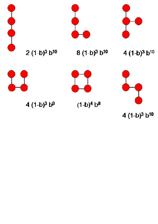
Figure 1: Cluster structures in two dimensional percolation. In this figure we show the 6 possible realizations of clusters of size 4 in a two dimensional grid. Circles denote nodes, straight lines denote active links. Together with each diagram we show the corresponding term in the sum $n_{4}$.

To include the isospin degree of freedom, a given node belonging to a cluster of size $A$ will be considered to be a proton with probability $p$. Then

$$n_{A}=\left[\underset{t}{\sum}g_{At}(1-b)^{a}b^{t}\right]\left[\underset{Z=0,A}{\sum}\alpha_{Z}p^{Z}(1-p)^{(A-Z)}\right]$$ (4)

with $\alpha_{Z}$ being the number of ways of building a cluster with $Z$ protons and $N=A-Z$ neutrons: $\alpha_{Z}={A!}/{N!Z!}$ The number of fragments per node with $A$ particles and $Z$ protons is then defined as:

$$n_{A,Z}=n_{A}[\alpha_{Z}p^{Z}q^{(A-Z)}]=n_{A}\alpha_{Z}p^{Z}q^{N}\ .$$ (5)

Focusing now on the isoscaling problem, the quantity of interest is the quotient:

$$R_{21}=\frac{Y_{2}(A,Z)}{Y_{1}(A,Z)}$$ (6)

With $Y_{2}$ representing the yield for the reaction involving the neutron rich nuclei.

For the percolation model, $R_{21}$ takes the form

$$R_{21}=\frac{[n_{A,Z}]_{2}}{[n_{A,Z}]_{1}}=\frac{p_{2}^{Z}q_{2}^{N}}{p_{1}^{Z}q_{1}^{N}}=\left(\frac{p_{2}}{p_{1}}\right)^{Z}\left(\frac{q_{2}}{q_{1}}\right)^{N}\ ,$$ (7)

in which all the geometrical and combinatorial terms cancel out and only the part related to the occupancy probabilities remains. In this way

$$R_{21}=\exp\left\{\ln\left[\left(\frac{p_{2}}{p_{1}}\right)^{Z}\left(\frac{q_{2}}{q_{1}}\right)^{N}\right]\right\}=\exp\left[N\ln\left(\frac{q_{2}}{q_{1}}\right)+Z\ln\left(\frac{p_{2}}{p_{1}}\right)\right]=\exp\left(\alpha N+\beta Z\right)\ .$$ (8)

Which is the standard expression of the isoscaling coefficient, but now with a clear microscopic interpretation for the isoscaling parameters $\alpha$ and $\beta$.

For finite lattices, it is convenient to study $R_{21}$ calculated in terms of the number of fragments $N_{A,Z}$ instead of the above derivation in terms of the number of fragments per node, $n_{A,Z}$. This can be achieved by using the above derived expressions for the constants $\alpha$ and $\beta$. Equation (7) can be rewritten as

$$R_{21}=\frac{\left[N_{A,Z}\right]_{2}}{\left[N_{A,Z}\right]_{1}}\approx\frac{A_{2}[n_{A,Z}]_{2}}{A_{1}[n_{A,Z}]_{1}}=\frac{A_{2}}{Z}\frac{Z}{A_{1}}\left(\frac{p_{2}}{p_{1}}\right)^{Z}\left(\frac{q_{2}}{q_{1}}\right)^{N}=\left(\frac{p_{2}}{p_{1}}\right)^{Z-1}\left(\frac{q_{2}}{q_{1}}\right)^{N}$$ (9)

where the probabilities have been approximated by $p_{i}\simeq Z/A_{i}$. This immediately yields the usual expression:

$$R_{21}=C\exp\left(\alpha N+\beta Z\right)$$ (10)

with $\alpha=\ln(q_{2}/q_{1})$, $\beta=\ln(p_{2/}p_{1})$ and $C=\exp[\ln(p_{1}/p_{2})]=p_{1}/p_{2}=A_{2}/A_{1}$

It should be kept in mind that the main assumptions in this derivation are that the probability $p$ is homogenous and that the number of fragments per node (per particle) can be approximated by the corresponding infinite size limit. We now turn to a numerical verification of these predictions.

III Numerical experiments

To explore the isoscaling phenomena in the framework of the above defined percolation model, two different types of calculations were performed: fixing the number of protons in the lattice, and using a fixed probability to assign the isospin to the nodes.

III.1 Fixed proton number

In this case, the $R_{21}$ was obtained using the yields of two lattices, one of size $6\times 6\times 6$, i.e. with $A=216$ nodes, and a second one of $7\times 7\times 7$ with $A=343$ nodes, both with the number of protons fixed to $108$. These grids, had, then, $Z=N=108$, and probabilities $p_{1}=0.5$ and $q_{1}=(1-p_{1})=0.5$ for the $6\times 6\times 6$ grid, and $Z=108$, $N=235$, $p_{2}=0.315$ and $q_{2}=(1-p_{2})=0.685$, for the $7\times 7\times 7$ grid.

For these probabilities, the isoscaling coefficients are $\alpha=\ln(0.6852/0.5)=\allowbreak 0.315\,$ and $\beta=\ln(0.3148/0.5)=\allowbreak-0.463$, and the constant $C=p_{1}/p_{2}=0.5/0.3148=\allowbreak 1.\,\allowbreak 588\,3$. The results of $200,000$ percolations of each of these grids are displayed in panel $a)$ of figure 2.

III.2 Fixed $p$ and $n$ occupancy probability

In this second case, the two isotopically different grids were constructed with the same sizes for both, but with two different protons and neutrons occupation probabilities. Several cases were studied.

First, $6\times 6\times 6$ grids were constructed using $p_{1}=0.5$ and $q_{1}=(1-p_{1})=0.5$ which yields a total number of protons (in average) of $\left\langle Z\right\rangle=108$ and $\left\langle N\right\rangle=108$, and $p_{2}=0.33$ and $q_{2}=(1-p_{2})=0.67$ which yields a total number of protons (in average) of $\left\langle Z\right\rangle=$ $72$ and $\left\langle N\right\rangle=$ $144$. In this case the coefficients are : $\alpha=\ln(0.67/0.5)=\allowbreak 0.292\,67,$ and $\beta=\ln(0.33/0.5)=\allowbreak-0.415\,52$. The results obtained from this numerical exercise are displayed in panel b) of figure 2; the fact that isoscaling is well reproduced by this purely geometrical model is obvious from this figure.

Next, to investigate size effects, a similar case was constructed using a smaller lattice of size $5\times 5\times 5$ with the same probabilities as in the previous case. The corresponding results are displayed in panel c) of figure 2; again the property of isoscaling is apparent.

Finally, to investigate the effect of different occupation probabilities on $R_{21}$, one more case was studied. In this case, a lattice of $6\times 6\times 6$ was populated with protons and neutrons according to the probabilities: $p_{1}=0.5$ and $q_{1}=(1-p_{1})=0.5$. For the neutron rich partner the probabilities used were $p_{2}=0.42$ and $q_{2}=(1-p_{2})=0.58$ which yields a total number of protons (on average) of $\left\langle Z\right\rangle=$ $91$ and $\left\langle N\right\rangle=$ $125$. In this case the coefficients are $\alpha=\ln(0.58/0.5)=\allowbreak 0.148\,42,$ and $\beta=\ln(0.42/0.5)=\allowbreak-0.174\,35$. The corresponding results are shown in panel d) of figure 2.

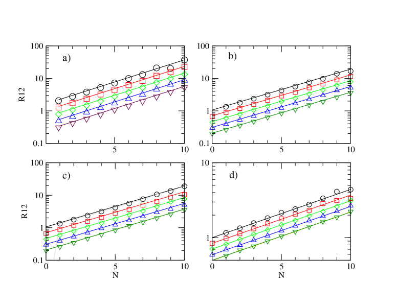
Figure 2: Isoscaling in percolation. Comparison of theoretical predictions for isoscaling in the nuclear percolation model and the corresponding results from numerical simulations. Lines denote theoretical predictions, symbols denote numerical simulations

For each of these cases $200,000$ configurations were generated. The bond breaking probability was chosen as $b=0.31$ in order to get good statistics in an ample range of masses. [Attempts with different values of the breaking probability $b$ demonstrated that the ratio $R_{21}$ is independent of $b$.] The figure also shows a comparison of the numerical results to the theoretical predictions of section III, lines denote theoretical predictions whereas symbols denote numerical simulations. The agreement between the theoretical predictions and the results of the simulations is remarkable.

IV Conclusions

We have studied the isoscaling phenomenon in the frame of percolation model. We have derived exact analytic expressions for the infinite case and approximate ones for the finite case. We have performed numerical simulations for not too big systems ($125,$ $216$ and $343$ “particles”) with different relative populations of N:Z. The excellent agreement between numerical simulations and theory indicate that isoscaling emerges from the simple assumption of fair sampling with homogeneous probabilities. On the other hand, this property can be seen as a minimum information approach, i.e. all configurations are equiprobable, as such this analysis can be interpreted in the frame of a maximum entropy approach. This indicates that the information about effects due, for example, to the asymmetry term in the equation of state, is in the absolute values of the parameters $\alpha$ and $\beta$, and not in the isoscaling property itself.

- (1) H. S. Xu, M. B. Tsang, T. X. Liu, X. D. Liu, W. G. Lynch, W. P. Tan, A. Vander Molen, G. Verde, A. Wagner, H. F. Xi, C. K. Gelbke, L. Beaulieu, B. Davin, Y. Larochelle, T. Lefort, R. T. de Souza, R. Yanez, V. E. Viola, R. J. Charity and L. G. Sobotka, Phys. Rev. Lett. 85, 716 (2000).
- (2) H. Johnston et al., Phys. Lett. B3715, 186 (1996).
- (3) R. Laforest et al., Phys. Lett. C59, 2567 (1999).
- (4) M. B. Tsang, C.K. Gelbke, X.D. Liu, W.G. Lynch, W.P. Tan, G. Verde, H.S. Xu, W. A. Friedman, R. Donangelo, S. R. Souza, C.B. Das, S. Das Gupta, D. Zhabinsky, Phys. Rev. C64, 054615 (2002).
- (5) M. B. Tsang, W. A. Friedman, C. K. Gelbke, W. G. Lynch, G. Verde and H. Xu, Phys. Rev. Lett. 86, 5023 (2001).
- (6) S. R. Souza, R. Donangelo, W. G. Lynch, W. P. Tan, and M. B. Tsang, Phys. Rev. C69, 031607 (2004).
- (7) C. B. Das, S. Das Gupta, X. D. Liu and M. B. Tsang, Phys. Rev., C64, 044608 (2001)
- (8) A. S. Botvina, O.V. Lozhkin, and W. Trautmann, Phys. Rev. C65, 044610 (2002).
- (9) A. Ono, P. Danielewicz, W. A. Friedman, W. G. Lynch, and M. B. Tsang, Phys. Rev. C68, 051601(R) (2003).
- (10) G.A. Souliotis et al., Phys. Rev. C68, 24605 (2003).
- (11) M. Veselsky, G.A. Souliotis and M. Jandel, Phys. Rev. C69 44607 (2004).
- (12) C. O. Dorso, C. Escudero, M. Ison, J. A. López, submitted to Phys. Rev. C (2005).
- (13) W. Bauer et al., Phys. Lett. 150B, 53 (1985); Nucl. Phys. A452, 699 (1986); Phys. Rev. C38, 1297 (1988).
- (14) X. Campi, J. Phys. A19, L917 (1986).
- (15) D. Stauffer and A. Aharony, ’Introduction to percolation theory’, Taylor & Francis (1992).
- (16) J. Elliott et al., Phys. Rev. C, (2000)
- (17) A. Barrañón, R. Cárdenas, C. O. Dorso, and J. A. López, Heavy Ion Physics 57, 1, (2003).