Level density of a Fermion gas: average growth, fluctuations, universality

Abstract

It has been shown by H. Bethe more than 70 years ago that the number of excited states of a Fermi gas grows, at high excitation energies $Q$, like the exponential of the square root of $Q$. This result takes into account only the average density of single particle (SP) levels near the Fermi energy. It ignores two important effects, namely the discreteness of the SP spectrum, and its fluctuations. We show that the discreteness of the SP spectrum gives rise to smooth finite–$Q$ corrections. Mathematically, these corrections are associated to the problem of partitions of an integer. On top of the smooth growth of the many–body density of states there are, generically, oscillations. An explicit expression of these oscillations is given. Their properties strongly depend on the regular or chaotic nature of the SP motion. In particular, we analyze their typical size, temperature dependence and probability distribution, with emphasis on their universal aspects.

1 Introduction

The main theoretical framework to understand the behavior of the density of states of a Fermionic system has been, and still is, the independent particle model. In the degenerate gas approximation, when the excitation energy of the gas is much smaller than the Fermi energy $\epsilon_{\scriptscriptstyle F}$, the excitation spectrum relies on the properties of the single–particle (SP) spectrum near $\epsilon_{\scriptscriptstyle F}$. In most theoretical calculations only the average SP density of states, $\overline{\rho}$, is taken into account. For a system of $A$ noninteracting fermions moving in a mean–field potential, the number of excited states of the many–body (MB) system contained in a small energy window $dQ$ at energy $Q$, $\rho_{\scriptscriptstyle MB}(A,Q)dQ$, is bethe

$$\rho_{\scriptscriptstyle MB}(A,Q)=\frac{1}{\sqrt{48}\ Q}\exp\left(2\sqrt{a\ Q}\right)\ ,\;\;\;\;\;\;\;\;\;\;a=\pi^{2}\overline{\rho}/6\ .$$ (1)

Here $Q$ is measured with respect to the ground state energy of the gas. For a given potential, $\overline{\rho}$ is in general a function of $A$. Besides the condition $Q\ll\epsilon_{\scriptscriptstyle F}$, this expression assumes that the excitation energy is large compared to the SP mean level spacing $\overline{\delta}=\overline{\rho}^{-1}$. For simplicity, and because our aim here is not to compare with experimental data, we ignore angular momentum conservation, isospin, etc.

After Bethe’s work, more accurate calculations of $\rho_{\scriptscriptstyle MB}$ were made bloch . Schematic shell corrections related to a periodic fluctuation of the SP density were computed in ros (see also bm ), introducing the so–called back-shifted Bethe formula. Several phenomenological modifications of Eq.(1) have been proposed to match the experimental results. These models take into account, for example, shell effects, pairing corrections and residual interactions gc ; ist ; krp ; abf , introducing a multitude of coexisting phenomenological parameterizations. The present status of the understanding do not allow to draw a clear theoretical picture of the functional dependence of $\rho_{\scriptscriptstyle MB}$ with $A$ and $Q$.

Our purpose is, within a SP picture, to further develop the theoretical analysis to include several important effects that are missing in Eq.(1). This presentation is based on the work reported in lmr .

There are different ways in which Eq.(1) can be improved. As mentioned before, it is the leading term of an expansion valid for a large number of particles $A$ and for high energies $Q$ (compared to the SP mean level spacing $\overline{\delta}$). For instance, assuming the gas is confined by a Woods–Saxon like mean field potential, then

$$\overline{\rho}=\frac{3}{2}\frac{A}{\epsilon_{\scriptscriptstyle F}}\;\Longrightarrow\;a=\frac{\pi^{2}}{4\epsilon_{\scriptscriptstyle F}}A\approx\frac{A}{15}\;{\rm MeV}^{-1}\ ,$$ (2)

where we used the approximation $\epsilon_{\scriptscriptstyle F}\approx 37$ MeV. This expression of $\overline{\rho}$ is the leading order term of an expansion in decreasing powers of $A$. Corrections to it can be incorporated by considering lower order terms in the Weyl series, that includes surface corrections, curvature corrections, etc bh . A similar expansion in decreasing powers of $A$ holds for the energy or mass of the nucleus (the liquid drop formula). As is well known, the coefficient of each term in the expansion of the energy obtained from a Fermi gas is not correct, since the renormalization due to interactions is out of the range of the model. Similarly, the coefficient $1/15$ in Eq.(2) does not give a good description of the average trend of the experimental data obtained from neutron resonances, which is closer to $1/8$ (cf Fig.1). Although of great interest, we will not discuss these $A$ corrections and their renormalization due to interactions, but concentrate on two other corrections that are within the scope of a noninteracting model. The first one (next section) leads to smooth lower order terms in the excitation energy $Q$. The second type of corrections incorporates oscillatory terms in $A$ and $Q$. These oscillations, superimposed to the smooth $A/8$ trend mentioned above, are clearly visible in the experimental data shown in Fig.1.

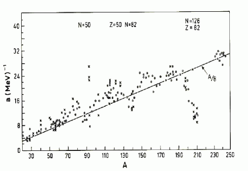
Figure 1: The parameter $a$ appearing in the Fermi gas level density formula as a function of the mass number $A$ (taken from Ref.bm ).

2 Discreteness of the spectrum: average behavior

The only property of the SP spectrum in Eq.(1) is the average density of levels $\overline{\rho}$. This approximation treats the SP spectrum as a continuum, and ignores the influence in the many–body density of states of the discreteness of the spectrum and of the exact position of the SP levels. One step beyond, that incorporates the discreteness but ignores the fluctuations, is to consider a locally perfectly regular SP spectrum (1D harmonic oscillator), given by the SP energies $\epsilon_{n}=n\delta$, where $n$ is an arbitrary integer, and $\delta$ is the distance between neighboring levels. The Fermi gas model consists of $A$ noninteracting fermions that occupy the equidistant levels, with occupation number 0 or 1. In the ground state the particles fill the lowest $A$ SP states. We restrict the analysis to the approximation $Q\ll\epsilon_{\scriptscriptstyle F}$, in which the number of excited particles is small compared to the total number $A$, and effects due to a finite number of particles can be ignored. In the excited states particles occupy SP levels above $\epsilon_{\scriptscriptstyle F}$, thus creating holes in the Fermi sea. The possible excited energies, measured with respect to the ground state energy, are $Q=m\delta$, where $m$ is an arbitrary positive integer. The excitation energies are thus trivial. The nontrivial information comes from the degeneracy of each of theses energies, since there are many different many–body configurations with the same excitation energy. The problem then is how to compute the degeneracy of each excited state of energy $Q=m\delta$.

Figure 2: Ground state (G.S., left column) and excited states of energy $Q/\delta=4$ (next five columns) of a gas of noninteracting fermions in a perfectly regular SP spectrum. Each excited state is identify with a decomposition of the excitation energy 4 as a sum of integers (bottom of each column).

The solution is obtained by realizing that the problem we are facing is exactly equivalent to a well known problem in mathematics, i.e. in how many different ways an integer can be decomposed as a sum of integers (partitions of an integer, $p(m)$). We will simply provide here a graphical illustration of this equivalence (Fig.2). Consider for example the case $m=4$, the argument easily generalizes to any $m$. $m=4$ can be decomposed as a sum of integers in 5 different ways (and thus $p(4)=5$): $1+1+1+1$, $2+1+1$, $2+2$, $3+1$ and $4$. As Fig.2 shows, each of these decompositions is in a one-to-one correspondence with one of the possible excited states of the Fermi gas of total energy $Q/\delta=4$. The ground state is shown on the left column. In the second column from the left four particles have been pushed one level up, hence the equivalence with $1+1+1+1$ (other mappings may be used as well). In the third column the upper particle was pushed up by two, the next two by one. Etc. As has been emphasized many times, there is also a (trivial) one–to–one correspondence between the partitions of an integer and the excited states of a gas of noninteracting bosons in a one–dimensional harmonic oscillator potential. In this case each integer in the decomposition of the excitation energy indicates the level occupied by one of the excited particles.

The partition of an integer grows very fast with $m$: it is 5 for $m=4$, whereas $p(200)=397999029388$ (this number was computed by hand by P. MacMahon in 1918). The generating function of $p(m)$ was obtained in 1753 by L. Euler. An explicit expression for $p(m)$ came much later, under the form of an asymptotic (exact) formula (initially obtained by Hardy and Ramanujan hr , improved and made rigorous later on by Rademacher rademacher ). To facilitate the comparison with more general approaches, we express the result in terms of $\overline{\rho}Q$, where here $\overline{\rho}=\delta^{-1}$ is the inverse of the exact spacing between neighboring levels. The first terms of the expansion are given by,

$$\log\left(\rho_{\scriptscriptstyle MB}^{\scriptscriptstyle HO}/\overline{\rho}\right)=\sqrt{\frac{2}{3}\pi^{2}\overline{\rho}\ Q}-\log\left(\sqrt{48}\ \overline{\rho}Q\right)-\ \frac{\pi^{2}+72}{24\sqrt{6}\pi}(\overline{\rho}Q)^{-\frac{1}{2}}-\left(\frac{3}{4\pi^{2}}-\frac{1}{24}\right)(\overline{\rho}Q)^{-1}+{\cal O}((\overline{\rho}Q)^{-\frac{3}{2}})\ .$$ (3)

We emphasize with the notation $\rho_{\scriptscriptstyle MB}^{\scriptscriptstyle HO}$ that this is the many–body density of states for a Fermi gas in a 1D harmonic oscillator spectrum. As expected, the first two terms of this equation reproduce Bethe’s formula. However, Eq.(3) goes much further: it is a truncation of the exact asymptotic expansion of the density of states, whose precision can be improved by adding further terms. Notice that all the terms in Eq.(3) are smooth functions of the excitation energy $Q$.

It is natural to ask about the relevance of Eq.(3) in realistic systems, where the true SP spectrum consists of discrete energy levels arranged, in most cases, with no particular order. Equation (3) clearly goes beyond Bethe’s result, since it describes the exact behavior of the many–body density of states of a gas of particles that occupy a discrete, perfectly regular arrangement of SP levels. It is therefore not unreasonable to expect that the result is valid for an arbitrary spectrum having the same average density $\overline{\rho}$, and that the effects of the fluctuations of the SP energy levels with respect to a perfectly regular arrangement come on top of it. Although we do not have for the moment an explicit proof of this statement, numerical simulations to be presented below seem to confirm this hypothesis.

3 Fluctuations

The exact dependence of $\rho_{\scriptscriptstyle MB}$ on $A$ and $Q$ is sensitive to the detailed arrangement of the SP energy levels around the Fermi energy. Strong deviations with respect to a regular spacing, with possible degeneracies, may be produced by the presence of symmetries of the confining self–consistent potential. These deviations induce, in turn, oscillations in the thermodynamic functions of the gas. Shell effects are therefore due to deviations (or bunching) of the SP levels with respect to a perfectly regular spectrum. The degeneracies of the electronic levels of an atom produced by the rotational symmetry are an extreme manifestation of level bunching. In general, in systems that have other symmetries, or have no symmetries at all, there will still be level bunching, but its importance will typically be minor. Therefore, depending on the presence or absence of symmetries, the shell effects may be more or less important. The level bunching, and more generally the fluctuations of the SP energy levels, are thus a very general phenomenon. The theories that describe those fluctuations make a neat distinction between systems with different underlying classical dynamics (e.g., regular or chaotic). Our understanding of these fluctuations and of their connections with the regular or chaotic nature of the SP motion has greatly increased in the last decades. For a recent review see sev .

Oscillations in the many–body density of states of nuclei are clearly visible in the experimental data available from neutron resonances as a function of the mass number $A$. The parameter $a$ extracted from the data, plotted in Fig.1, shows oscillations around an average growth ($A/8$). The effective description of the oscillations through the parameter $a$ is an artifact of the analysis, since the Fermi gas model relates $a$ to $\overline{\rho}$, a smooth function. As we will see below, the theoretical analysis leads to oscillatory corrections that enter as an additional term in the exponent of $\rho_{\scriptscriptstyle MB}$, and thus cannot in general be interpreted as an effective $a$.

There are two distinct and important scales to describe the SP fluctuations. The first one, the smallest one, is the mean spacing between SP energy levels $\overline{\delta}$. The fluctuations of the SP energy levels on that scale have been shown to be, for a large class of systems, universal. Their statistical properties are described by uncorrelated sequences for integrable systems, and by random matrix theory in chaotic ones. The second relevant energy scale is $E_{c}=h/\tau_{\rm min}$, where $\tau_{\rm min}$ is of the order of the time of flight across the system (a precise definition will be given below). For $A$ large, the ratio $g=E_{c}/\overline{\delta}$ is much larger than one (for instance, $g\sim A^{2/3}$ in a three dimensional cavity). In contrast to the fluctuations on scales $\overline{\delta}$, the fluctuations on scales $E_{c}$ are long range modulations of the SP spectrum whose structure and amplitude are system specific. There is therefore no universality on this scale.

For an arbitrary SP spectrum the computation of the density of excited states of a fermionic system is a difficult combinatorial problem for which no exact solution is known. What we are seeking here are the variations of the MB density of states due to fluctuations of the SP spectrum with respect to a perfectly ordered spectrum, described in the previous section. An explicit formula that includes these effects has been obtained recently lmr . The result, obtained from a saddle point approximation of an inverse Laplace transform of the MB density, takes the form lmr

$$\rho_{\scriptscriptstyle MB}(A,Q)=\frac{1}{\sqrt{48}\ Q}\exp\left\{2\sqrt{a\ Q}+\sqrt{\frac{a}{Q}}\left[\widetilde{\cal E}(\mu,0)-\widetilde{\cal E}(\mu,T)\right]\right\}\ .$$ (4)

The function $\widetilde{\cal E}(\mu,T)$ is the fluctuating part of the energy of the gas at chemical potential $\mu$ and temperature $T$, defined as follows. The energy is, as usual, given by

$${\cal E}(\mu,T)=\int d\epsilon\ \epsilon\ \rho(\epsilon)\left[1+{\rm e}^{(\epsilon-\mu)/T}\right]^{-1}\ ,$$ (5)

where the function $\rho(\epsilon)$ is the SP density of states defined by the SP energies $\epsilon_{i}$

$$\rho(\epsilon)=\sum_{i}\delta(\epsilon-\epsilon_{i})\ .$$

The SP density of states is usually decomposed into a part $\overline{\rho}$ that has a smooth dependence on the energy $\epsilon$ plus another contribution $\widetilde{\rho}$ that describes the deviations with respect to the smooth behavior. The fluctuating part of the energy is defined as

$$\widetilde{\cal E}(\mu,T)={\cal E}(\mu,T)-\int d\epsilon\ \epsilon\ \overline{\rho}(\epsilon)\left[1+{\rm e}^{(\epsilon-\mu)/T}\right]^{-1}\ .$$ (6)

In Eq. (4) the arguments of $\widetilde{\cal E}$ are functions of $A$ and $Q$, $\mu=\mu(A,Q)$ and $T=T(A,Q)$. These two functions are determined by inversion of the equations

$$A = {\cal N}(\mu,T)\ ,$$ (7)

$$Q = {\cal E}(\mu,T)-{\cal E}(\mu,0)\ .$$

The function ${\cal N}(\mu,T)=\int d\epsilon\ \rho(\epsilon)\left[1+{\rm e}^{(\epsilon-\mu)/T}\right]^{-1}$ is the particle number. We are ignoring here (small) variations of the chemical potential with temperature. To lowest order, in which only the average behavior of the energy and of the particle number is taken into account, the second equation in (7) leads to the usual relation between temperature and excitation energy

$$T\approx\sqrt{\frac{Q}{a}}\ ,$$ (8)

and $\mu$ is simply a function of $A$, $\mu=\mu(A)$. For instance, for a Fermi gas in a 3D cavity of volume $V$ and particle mass $m$,

$$\mu\approx\frac{2\pi\hbar^{2}}{m}\left(\frac{3\sqrt{\pi}A}{4V}\right)^{2/3}\ .$$ (9)

Equation (4) shows that, superimposed to the smooth growth of the density described by Eq.(1), there are oscillatory corrections in the exponent of the density of states. These corrections are directly related to energy fluctuations of the system.

The oscillatory nature of the new corrections is clearly displayed through a semiclassical theory, that expresses the quantum properties of the fermion gas in terms of classical solutions of the SP equations of motion. In this approach $\widetilde{\cal E}(\mu,T)$ is written as a sum over the classical periodic orbits of the mean–field potential sm ; lm3 ; sev

$$\widetilde{\cal E}(\mu,T)=2\hbar^{2}\sum_{p}\sum_{r=1}^{\infty}\frac{A_{p,r}~{}\kappa(r~{}\tau_{p}/\tau_{\scriptscriptstyle T})}{r^{2}~{}\tau_{p}^{2}}\cos\left(r\ S_{p}/\hbar+\nu_{p,r}\right)\ .$$ (10)

Each orbit is characterized by its action $S_{p}$, stability amplitude $A_{p,r}$, and Maslov index $\nu_{p,r}$. $\tau_{p}$ is the period of the periodic orbit, and $\kappa(x)=x/\sinh(x)$ is a temperature factor that introduces the time scale $\tau_{\scriptscriptstyle T}=\hbar/(\pi T)$ conjugate to the temperature. This expression describes the departures of ${\cal E}$ with respect to its mean behavior due to the fluctuations of the SP spectrum. The behavior of $\widetilde{\cal E}$ strongly depends on whether $\mu$ or $T$ (or $A$ or $Q$) are varied. A temperature variation modifies the prefactors of the summands in $\widetilde{\cal E}$ (through the function $\kappa$), and therefore produces gentle variations of the fluctuating part in the exponent of the density of states

$$\widetilde{{S}}(A,Q)=\sqrt{\frac{a}{Q}}\left[\widetilde{\cal E}(\mu,0)-\widetilde{\cal E}(\mu,T)\right]\ .$$ (11)

In contrast, $A_{p,r}$, $\tau_{p}$ and $S_{p}$ depend on $\mu$ (and therefore on $A$). For large values of $\mu$, $S_{p}\gg\hbar$ and the dominant variation with the particle number (or any other parameter that modifies the actions) comes from the argument of the cosine function in $\widetilde{\cal E}$. Rapid oscillations of $\widetilde{{S}}$ are therefore generically expected when the number of particles is varied.

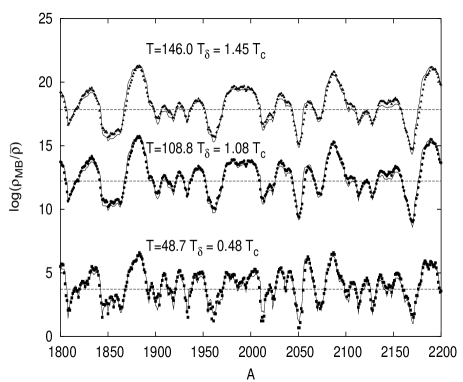
Figure 3: The logarithm of the many-body density of states of $A$ noninteracting fermions in a rectangular billiard of sides $a=\sqrt{(1+\sqrt{5})/2}$ and $b=a^{-1}$. The value of $g$ is 100. Dots: numerical computation at three different excitation energies; solid curves: theoretical prediction (12); dashed curves: smooth part Eq.(3).

For a given mean field potential there exists an infinite number of periodic orbits $p$. The spectrum of periods $\tau_{p}$ has no upper bound. It has, however, a lower bound, given by the period $\tau_{\rm min}$ of the shortest periodic orbit. Since $\tau_{\rm min}$ is usually the smallest characteristic time scale in the system, it determines the largest energy scale $E_{c}=h/\tau_{\rm min}$ in which modulations (bunching) of the SP energy levels occur

If the classical periodic orbits are known in a particular system, the corrections can be computed explicitly. The periodic–orbit sum is dominated by the short orbits, and rapidly gives a good approximation of the result. To illustrate our findings we have tested some of the predictions by a direct numerical counting of the MB density of states in a particular system. Figure 3 shows the results obtained for a gas of about 2000 fermions contained in a two–dimensional rectangular cavity, an integrable system. For each number of particles we compute the MB density of states at three different temperatures, measured in units of

$$T_{\delta}=\overline{\delta}/2\pi^{2}\;\;{\rm and}\;\;T_{c}=E_{c}/2\pi^{2}\ .$$

The theoretical curve is computed according to the expression

$$\log(\rho_{\scriptscriptstyle MB}/\overline{\rho})=\log(\rho_{\scriptscriptstyle MB}^{\scriptscriptstyle HO}/\overline{\rho})+\widetilde{{S}}(A,Q)\ ,$$ (12)

where $\widetilde{{S}}$ is calculated from the periodic orbits of the rectangle.

If the smooth corrections to the density of Eq.(3) are not included, and only the result of Bethe is used, a systematic deviation is observed in the average behavior of $\rho_{\scriptscriptstyle MB}$ between theory and numerics. Although the theoretical analysis of Ref.lmr does not include those corrections, the numerical results seem to indicate that their validity goes beyond the simple 1D harmonic oscillator spectrum. Notice the extremely good accuracy of Eq.(12), either for the average value of the density as well as for the fluctuations. Notice also that the typical size of the fluctuations can be quite important (it is of the order of the average for the lowest excitation energy computed).

4 Statistical analysis of the fluctuations: universality

Equation (12) decomposes the exponent of the density of states into a smooth part (given by the Hardy–Ramanujan result) plus oscillatory contribution, $\widetilde{{S}}(A,Q)$, associated in a semiclassical theory to a sum over periodic orbits. $\widetilde{{S}}(A,Q)$ relates the shell corrections in the MB density of states to the fluctuations of the energy of the gas. $\widetilde{\cal E}$ depends on temperature only through the function $\kappa$ (cf Eq.(10)). The effect of this function is to exponentially suppress the contribution of periodic orbits whose period $\tau_{p}\gg\tau_{\scriptscriptstyle T}$ ruj ; lm3 . Since there is no suppression at $T=0$ (because $\tau_{\scriptscriptstyle T}\rightarrow\infty$), only orbits whose period $\tau_{p}\stackrel{{\scriptstyle>}}{{\scriptstyle\sim}}\tau_{\scriptscriptstyle T}$ contribute to the difference $\widetilde{\cal E}(\mu,0)-\widetilde{\cal E}(\mu,T)$. At temperatures such that $\tau_{\scriptscriptstyle T}\ll\tau_{\rm min}$, the term $\widetilde{\cal E}(\mu,T)$ becomes exponentially small, and only $\widetilde{\cal E}(\mu,0)$ remains. The shell correction $\widetilde{{S}}(A,Q)$ therefore decays as $T^{-1}$ at $T\gg T_{c}$. This decay contrasts with the more common exponential damping observed in other thermodynamic quantities lm3 .

A clearer picture of how the fluctuations behave may be obtained through a statistical analysis. The most simple property of the fluctuations is $\langle\widetilde{{S}}\rangle=0$, where the brackets denote an average over a suitable chemical potential (or particle number) window. This result is valid only to first order in the expansion leading to Eq.(4) lmr ; it can be shown that higher order terms contribute to a non–zero average. The next non–trivial statistical property is the variance $\langle\widetilde{{S}}^{2}\rangle$, that may be computed using Eq.(10). The result is $\langle\widetilde{{S}}^{2}\rangle=(1/2)\int_{0}^{\infty}dx\ K(x,x_{\rm H})\left[1-\kappa(x)\right]^{2}/x^{4}$, where $K(x,x_{\rm H})$ is the rescaled form factor of the SP spectrum (cf Eq.(36) in Ref.lm3 ). The latter function depends on the rescaled Heisenberg time $x_{\rm H}=h\overline{\rho}/\tau_{\scriptscriptstyle T}$. It describes system–dependent features for $x$ of the order of $x_{\rm min}=\tau_{\rm min}/\tau_{\scriptscriptstyle T}$, while it is believed to be universal for $x\gg x_{\rm min}$. The universality class depends on the regular or chaotic nature of the dynamics, and on its symmetry properties.

Taking into account the basic properties of $K(x,x_{\rm H})$, in chaotic systems three different regimes for $\langle\widetilde{{S}}^{2}\rangle$ as a function of temperature are found lmr (remember the relation (8) between $T$ and $Q$):

• Low temperatures $T\ll T_{\delta}$. In this regime

  $$\langle\widetilde{{S}}^{2}\rangle=c_{4}T/(2T_{\delta})\ ,$$ (13)

  where $c_{4}=0.0609...$ is the value at $k=4$ of the constant

  $$c_{k}=\int_{0}^{\infty}\frac{d\ x}{x^{k}}\left[1-\frac{x}{\sinh x}\right]^{2}\ .$$ (14)

• Intermediate temperatures $T_{\delta}\ll T\ll T_{c}$. In this regime the size of the fluctuations saturates at a universal constant

  $$\langle\widetilde{{S}}^{2}\rangle=c_{3}/\beta\ ,$$ (15)

  where $c_{3}=0.1023\ldots$ and $\beta=1(2)$ for systems with (without) time–reversal invariance.

• High temperatures $T\gg T_{c}$. The size of the fluctuations decreases with excitation energy,

  $$\langle\widetilde{{S}}^{2}\rangle=\langle\widetilde{\cal E}^{2}(\mu,0)\rangle[1-8\ {\rm e}^{-T/T_{c}}]/T^{2}\ .$$ (16)

  After an exponential transient, a power–law decay $\langle\widetilde{{S}}^{2}\rangle^{1/2}\propto T^{-1}$ is thus obtained.

The situation is different in integrable systems, where only two regimes are found. At low temperatures the result is identical to that of chaotic systems. The linear growth at low temperatures is thus totally universal and independent of the system. The difference is that in integrable systems the growth extends up to much higher temperatures, $T\approx T_{c}$, without saturation. At that temperature the variance of the fluctuations is of order $g$. In integrable systems, the maximum amplitude of the fluctuations is therefore reached at $T\approx T_{c}$, and its typical size is much larger than in chaotic systems. At high temperatures $T\gg T_{c}$ the decay is almost identical to that of chaotic systems (the coefficient 8 is replaced by a 12). A schematic representation of the temperature dependence of the variance of the fluctuations for chaotic and integrable systems is given in Fig.4.

Figure 4: Schematic representation of the temperature dependence of the variance of the fluctuations in chaotic and integrable systems. In each class, the behavior is universal in the regime $T\ll T_{c}$.

It has been shown lm3 that $\widetilde{\cal E}(\mu,T)$ is dominated, at any $T$, by the shortest classical periodic orbits. In contrast, the difference $\widetilde{\cal E}(\mu,0)-\widetilde{\cal E}(\mu,T)$ depends on orbits whose period $\tau_{p}\stackrel{{\scriptstyle>}}{{\scriptstyle\sim}}\tau_{\scriptscriptstyle T}$. For temperatures $T\ll T_{c}$ the statistical properties of these orbits are universal, and correspondingly the probability distribution function of $\widetilde{{S}}$ is expected to be universal, in the sense that at a given temperature it should only depend on the nature of the underlying classical dynamics (regular or chaotic), and the symmetries of the system. This statement is supported by the fact that in the limit $T\rightarrow 0$, $\widetilde{{S}}\approx-\partial\widetilde{\cal E}(\mu,T)/\partial T$. The probability distribution of the latter quantity was studied in Ref.lm3 ; it was shown that it coincides at low temperatures with that obtained from a Poisson spectrum for integrable systems and from a random matrix spectrum for chaotic ones. This confirms the universality of the distribution at low temperatures. As the temperature is raised, the universality of the probability distribution of $\widetilde{{S}}$ will be lost for temperatures of the order or greater than $E_{c}$, where system specific features (i.e., short periodic orbits) are revealed. In this respect, the decay (16) is only indicative. Its exact form depends on the details of the short periodic orbits spectrum, treated here only through a rough approximation.

5 Concluding remarks

Two improvements with respect to Bethe’s formula of $\rho_{\scriptscriptstyle MB}$ have been discussed. The first one incorporates the discreteness of the SP spectrum by considering a set of equidistant SP states (1D harmonic oscillator). The exact many–body density of states is obtained by mapping the problem to the computation of the number of decompositions of an integer as a sum of integers. The exact formula adds finite–$Q$ corrections to the asymptotic result. Although a proof is missing, numerical simulations suggest that the range of validity of this result extends beyond the 1D harmonic oscillator spectrum to any spectrum, in the sense that it describes with good accuracy the smooth part of the growth of $\rho_{\scriptscriptstyle MB}$ in systems with an arbitrary SP spectrum (cf Fig.3).

Beyond the smooth behavior, the second improvement concerns the fluctuations or shell effects in $\rho_{\scriptscriptstyle MB}$. In a semiclassical theory, each periodic orbit has been shown to contribute to $\log(\rho_{\scriptscriptstyle MB}/\overline{\rho})$ with a fluctuating term as a function of the number of particles $A$, of wavelength

$$\Delta A=\frac{h/\tau_{p}}{\overline{\delta}}\ .$$

At low excitation energies long orbits contribute to the fluctuations while short ones are exponentially suppressed, leading to wild oscillations and universality of their statistical properties. As the temperature increases, the situation is reversed, long orbits are exponentially suppressed while short orbits come into play. At $T=T_{c}$, oscillations of wavelength of order $\Delta A=E_{c}/\overline{\delta}=g$ are predicted. These oscillations are clearly visible, with the correct wavelength, in Fig.3. With the raise of the short periodic orbits as $T$ increases, the universality of the statistical properties of the fluctuations disappears for $T$ of the order or higher than $T_{c}$.

Concerning the typical size of the oscillations, a nontrivial dependence as a function of excitation energy (or temperature) was found. The results are summarized in Fig.4. The behavior is quite different in chaotic and integrable systems. At low temperatures the variance grows linearly with $T$ in all cases. However, a plateau is rapidly reached at $T=T_{\delta}$ in chaotic systems, whereas the amplitude of the fluctuations continue to grow in regular ones. At $T=T_{c}$ the differences reaches its maximum amplitude, where the variance in regular systems is $g$ times larger than in chaotic ones (remember, moreover, that $g\sim A^{2/3}$ in a three dimensional cavity, so that the difference increases with an increasing number of particles). At this point the situation is similar to what was found for the ratio of the variance of the fluctuations of the nuclear mass due to regular and chaotic motion bl . At $T\gg T_{c}$ the variance decreases as $T^{-2}$ for both types of dynamics. The validity of the results discussed here in the analysis and interpretation of the experimental data on the nuclear level density will be presented elsewhere.

References

- (1) H. A. Bethe, Phys. Rev., 50, 332 (1936).
- (2) C. Bloch, Phys. Rev., 93, 1094 (1954).
- (3) N. Rosenzweig, Phys. Rev., 108, 817 (1957).
- (4) A. Bohr and B. R. Mottelson, Nuclear Structure, Vol.I, Benjamin, Reading, Massachusetts, 1969.
- (5) A. Gilbert and A. G. W. Cameron, Can. J. Phys., 43, 1446 (1965).
- (6) A. V. Ignatyuk, G. N. Smirenkin, and A. S. Tishin, Sov. J. Nucl. Phys., 21, 255 (1975).
- (7) K. Kataria, V. S. Ramamurthy, and S. S. Kapoor, Phys. Rev. C, 18, 549 (1978).
- (8) Y. Alhassid, G. F. Bertsch, and L. Fang, Phys. Rev. C, 68, 044322 (2003).
- (9) P. Leboeuf, A. G. Monastra and A. Relaño, Phys. Rev. Lett., 94, 102502 (2005).
- (10) H. P. Baltes and E. R. Hilf: Spectra of Finite Systems, Bibliographisches Institut-Wissenschaftsverlag, Mannheim, 1976.
- (11) G. H. Hardy and S. Ramanujan, Proc. London Math. Soc., 17, 75 (1918).
- (12) H. Rademacher, Proc. London Math. Soc., 43, 241 (1937).
- (13) P. Leboeuf, Regularity and chaos in the nuclear masses, Lectures delivered at the VIII Hispalensis International Summer School, Sevilla, Spain, June 2003 (to appear in Lecture Notes in Physics, Springer–Verlag, Eds. J. M. Arias and M. Lozano); nucl-th/0406064.
- (14) V. M. Strutinsky and A. G. Magner, Sov. J. Part. Nucl. 7 (1976) 138.
- (15) P. Leboeuf and A. G. Monastra, Ann. Phys., 297, 127 (2002).
- (16) K. Richter, D. Ullmo and R. Jalabert, Phys. Rep., 276, 1 (1996).
- (17) O. Bohigas and P. Leboeuf, Phys. Rev. Lett., 88, 092502 (2002); 88, 129903 (2002).