Hydrodynamical evolution of dissipative QGP fluid

Abstract

In the framework of the Mueller-Israel-Stewart theory of dissipative fluid dynamics, we have studied the space-time evolution of a QGP fluid. For simplicity, we have considered shear viscosity only and neglected bulk viscosity and heat conductivity. Shear viscosity opposes the expansion and cooling of the fluid. As a result, the lifetime of the fluid is extended. We also find that the parton $p_{T}$ distribution is considerably flattened.

1 Introduction

One of the primary goals of relativistic heavy ion collisions is the creation and detection of the (lattice QCD [1]) predicted deconfined phase of quarks and gluons. Experiments at RHIC, BNL, gave strong indications of QGP formation in central Au+Au collisions [2]. Hydrodynamics provides a simple, intuitive dynamic description of relativistic heavy ion collisions. Most of the experimental data on soft hadron production at RHIC are well described by ideal hydrodynamics. However, some problems remain. For example, one of the most important signals of collectivity, the elliptic flow, saturates beyond $p_{T}\sim 1.5{-}2$ GeV/$c$ while ideal hydrodynamics predicts a continuous increase with $p_{T}$ [3].

Ideal hydrodynamic may not give an accurate description of the early stage of the collision. In the early stages of collision, particle momenta are predominantly in the beam direction, while ideal hydrodynamic assumes a locally isotropic distribution. The anisotropy in the momentum distribution will give rise to shear viscous stress. Other dissipative effects, e.g. bulk viscosity and heat conduction can also affect the hydrodynamic evolution of QGP. Unlike ideal flow, non-ideal flow generates entropy. The space-time evolution is also changed.

Relativistic theories for dissipative fluid dynamics were formulated long ago [4, 5, 6]. In early formulations, called 1st order theories [4, 5], the entropy 4-current contained terms of first order in the dissipative fluxes; these had the undesirable feature of violating causality. This is corrected in so-called 2nd order theories, due to Grad, Mueller and Israel and Stewart [6]. In 2nd order theories, the entropy 4-current contains terms of 2nd order in the dissipative fluxes. The space of thermodynamic variables is extended to include the dissipative fluxes, and relaxation equations for these dissipative fluxes are obtained from the positivity condition for entropy production $\partial_{\mu}s^{\mu}\geq 0$.

Up to now, only a few authors have considered the effects of dissipation in relativistic heavy ion collisions [7, 8, 9, 10, 11, 12, 13]. Most of these studies considered one dimensional systems using 1st order theories. Only recently 2nd order theories have been implemented numerically [10, 12, 13]. In the present paper, using the causal 2nd order theory of dissipative fluid dynamics, we study the effect of shear viscosity on the space-time evolution of a QGP fluid. The paper is organized as follows: In Section II, we present the equations for 2nd order dissipative hydrodynamics. Our choice of equation of state, transport coefficients and initial conditions is described in Section III. Results for the space-time evolution of the QGP fluid, with and without dissipation, are presented Section IV. Conclusions are drawn in Section VI.

2 Equations for causal dissipative hydrodynamics

We consider a QGP fluid in the central rapidity region, with zero net baryon density and chemical potential, $n_{B}=0,\ \mu_{B}=0$. We neglect the effects of heat conduction ($\mu_{B}=0$) and bulk viscosity (massless particles) and account only for shear viscosity. We work in the Landau-Lifshitz energy frame.

The energy-momentum tensor, including the shear viscous pressure tensor $\pi^{\mu\nu}$, is written as [6]

$$T^{\mu\nu}=(\varepsilon+p)u^{\mu}u^{\nu}-pg^{\mu\nu}+\pi^{\mu\nu}$$ (1)

where $\varepsilon$ is the energy density, $p$ is the hydrostatic pressure, and $u$ is the hydrodynamic 4-velocity, normalized by $u^{\mu}u_{\mu}=1$. $T^{\mu\nu}$ satisfies the energy-momentum conservation law

$$\partial_{\mu}T^{\mu\nu}=0.$$ (2)

In the Israel-Stewart theory of dissipative fluids [6], the dissipative fluxes are treated as independent thermodynamic variables which satisfy kinetic relaxation equations. The transport (relaxation) equations for the shear viscous pressure read

$$\beta_{2}D\pi^{\mu\nu}=-\frac{1}{2\eta}\pi^{\mu\nu}+\nabla^{\left\langle\mu\right.}u^{\left.\nu\right\rangle}$$ (3)

where $D=u^{\mu}\partial_{\mu}$ is the convective time derivative. $\eta$ is the shear viscosity coefficient. $\beta_{2}$ is related to relaxation time by $\tau_{\pi}=2\eta\beta_{2}$. The angular bracket in $\nabla^{\left\langle\mu\right.}u^{\left.\nu\right\rangle}$ is defined as

$$\nabla^{\left\langle\mu\right.}u^{\left.\nu\right\rangle}=\frac{1}{2}[\nabla^{\mu}u^{\nu}+\nabla^{\nu}u^{\mu}]-\frac{1}{3}\Delta^{\mu\nu}\partial_{\sigma}u^{\sigma},$$ (4)

where $\nabla^{\mu}=\partial^{\mu}-u^{\mu}D$ is the transverse gradient operator and $\Delta^{\mu\nu}=g^{\mu\nu}-u^{\mu}u^{\nu}$ is the projector orthogonal to the flow velocity $u^{\mu}$.

The viscous pressure tensor $\pi^{\mu\nu}$ is symmetric and traceless $\pi^{\mu\nu}=\pi^{\nu\mu}$ and $\pi^{\mu}_{\mu}=0$. Furthermore, it is transverse to the hydrodynamic 4-velocity, $u_{\mu}\pi^{\mu\nu}=0$. Thus it has 5 independent components.

There are 10 unknowns ($\varepsilon$, $p$, three components of the hydrodynamic velocity $u$, and 5 viscous pressure components) and 9 equations (4 energy-momentum conservation equations and 5 transport equations for the independent components of $\pi^{\mu\nu}$. The system is closed by the equation of state $p=p(\varepsilon)$. We assume longitudinal boost-invariance and cylindrical symmetry in the transverse direction. These additional symmetries reduce the independent variables to four (energy density $\varepsilon$, radial velocity $v_{r}$ and two components, say $\pi^{rr}$ and $\pi^{\phi\phi}$, of the viscous pressure tensor). In $(\tau,r,\phi,\eta)$ coordinates, the hydrodynamic and relaxation equations read (see appendix)

$$\partial_{\tau}\tilde{T}^{\tau\tau}+\partial_{r}\left(v_{s}\tilde{T}^{\tau\tau}\right) = -\frac{\tilde{p}-\tilde{\pi}^{rr}/\gamma^{2}-r^{2}\tilde{\pi}^{\phi\phi}}{\tau},$$ (5)

$$\partial_{\tau}\tilde{T}^{\tau r}+\partial_{r}\left(v_{r}\tilde{T}^{\tau r}\right) = \frac{\tilde{p}+r^{2}\pi^{\phi\phi}}{r}-\partial_{r}\left(\tilde{p}+\frac{\tilde{\pi}^{rr}}{\gamma^{2}}\right),$$ (6)

$$\partial_{\tau}\pi^{rr}+v_{r}\partial_{r}\pi^{rr} = -\frac{1}{\tau_{\pi}\gamma}\left(\pi^{rr}-2\eta\nabla^{\left\langle r\right.}u^{\left.r\right\rangle}\right),$$ (7)

$$\partial_{\tau}\pi^{\phi\phi}+v_{r}\partial_{r}\pi^{\phi\phi} = -\frac{1}{\tau_{\pi}\gamma}\left(\pi^{\phi\phi}-2\eta\nabla^{\left\langle\phi\right.}u^{\left.\phi\right\rangle}\right).$$ (8)

where $\tilde{A}^{\mu\nu}=r\tau A^{\mu\nu}$, $\tilde{p}=r\tau p$ and $v_{s}=T^{\tau r}/T^{\tau\tau}$.

The four equations are solved simultaneously using the SHASTA-FCT algorithm [14]. At each time step, we obtain the energy density $\varepsilon$ and radial velocity $v_{r}$ from $T^{\tau\tau}$, $T^{\tau r}$, and $\pi^{rr}$ by iteratively solving (in analogy to the ideal fluid case [15])

$$v_{r}=\frac{T^{\tau r}}{T^{\tau\tau}+p(\varepsilon)+\pi^{rr}/\gamma^{2}},\qquad\varepsilon=T^{\tau\tau}-v_{r}T^{\tau r}.$$ (9)

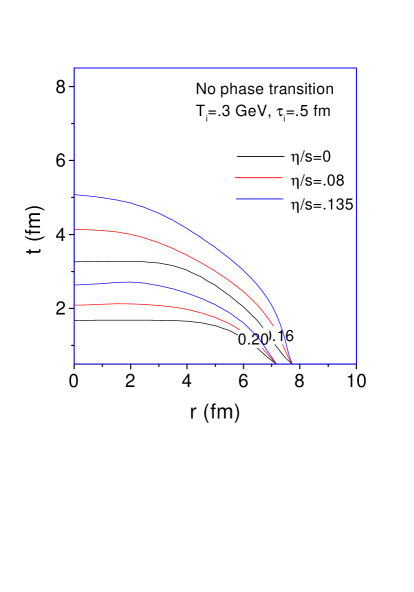
Figure 1: Contours of constant temperature in the $r{-}\tau$ plane for ideal and non-ideal hydrodynamic evolution, using $T_{i}{\,=\,}0.3$ GeV at $\tau_{i}{\,=\,}0.5$ fm/$c$.

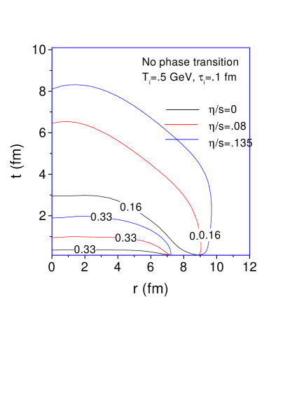
Figure 2: Contours of constant temperature in the $r{-}\tau$ plane for ideal and non-ideal hydrodynamic evolution, using $T_{i}$=0.5 GeV at $\tau_{i}{\,=\,}0.1$ fm/$c$.

3 Equation of state, transport coefficient and initial conditions

The equation of state is one of the important inputs for hydrodynamics. It is the link between the macroscopic and microscopic world. In this exploratory work, we have used a simple equation of state, $p=\frac{1}{3}\varepsilon$, with $\varepsilon=aT^{4}$, $a=(16+\frac{21}{2}N_{f})\frac{\pi^{2}}{30}$.

In classical kinetic theory, explicit expressions can be obtained for the viscosity coefficient $\eta$ and the relaxation time $\tau_{\pi}$ in terms of the collision term. For a strongly coupled QGP, neither $\eta$ or $\tau_{\pi}$ are known. We treat them as phenomenological parameters. For guidance, we use perturbative [17, 16] and AdS/CFT [18] estimates for $\eta$, respectively, and a kinetic theory estimate [6] for $\tau_{\pi}$.

The shear viscosity coefficient $\eta$ for hot QCD was determined perturbatively to leading logarithmic accuracy in [16, 17]. For $\alpha_{s}\approx 0.5$ the result in [17] gives

$$\frac{\eta}{s}=0.135.$$ (10)

Recently the shear viscosity was also evaluated in a strongly coupled gauge theory ($N=4$ SUSY YM theory), using the AdS/CFT correspondence [18]. The corresponding AdS/CFT estimate of shear viscosity is

$$\frac{\eta}{s}=0.08$$ (11)

In kinetic theory, in the Boltzmann gas approximation, the relaxation time is estimated as $\tau_{\pi}=2\eta\beta_{2}=2\eta\,\frac{3}{4p}$ [6]..

For the initial energy density distribution in the transverse plane, we use the Woods-Saxon parameterisation:

$$\varepsilon(r)=\frac{\varepsilon_{0}}{1+e^{\frac{r-R}{a}}},$$ (12)

with $R{\,=\,}6.4$ fm, $a{\,=\,}0.54$ fm. This is not very realistic, but facilitates comparison with the results of [13]. ($\varepsilon_{0}{\,=\,}aT_{i}^{4}$ is the central energy density at initial time $\tau{\,=\,}\tau_{i}$.) We have considered two sets of initial conditions: (i) $T_{i}{\,=\,}0.3$ GeV and $\tau_{i}{\,=\,}0.5$ fm/$c$, and (ii) $T_{i}{\,=\,}0.5$ GeV and $\tau_{i}{\,=\,}0.1$ fm/$c$. Both sets have similar total initial entropy content.

We also assume that at the initial time $\tau_{i}$ the radial velocity vanishes ($v_{r}(r)=0$).

For the non-ideal fluid, initial viscous pressures, $\pi^{rr}$ and $\pi^{\phi\phi}$ are required. Even though $v_{r}$ and its derivatives are zero initially, due to the Bjorken longitudinal motion the stress tensor is not zero: $\nabla^{\left\langle r\right.}u^{\left.r\right\rangle>}=r^{2}\nabla^{\left\langle\phi\right.}u^{\left.\phi\right\rangle>}=\frac{1}{3\tau_{i}}$. We assume that at initial time $\tau_{i}$, the viscous pressure components are fully relaxed to the Bjorken scaling expansion values,

$$\pi^{rr}=r^{2}\pi^{\phi\phi}=\frac{2\eta}{3\tau_{i}}.$$ (13)

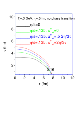
Figure 3: Freeze-out surface at $T_{f}{=}160$ MeV for different initial viscous pressures.

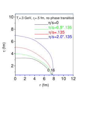
Figure 4: Freeze-out surface at $T_{f}{=}160$ MeV for different shear viscosities $\eta$.

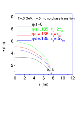
Figure 5: Freeze-out surface at $T_{f}{=}160$ MeV for different relaxation times $\tau_{\pi}$.

4 Results

4.1 Space-time evolution of ideal and non-ideal QGP

With have solved the hydrodynamic equation for ideal and non-ideal fluids, with identical initial conditions. We do not invoke a phase transition. The initial QGP evolves without undergoing phase transition until it freezes out at a an assumed freeze-out temperature $T_{f}{\,=\,}160$ MeV.

In Figs. 2 and 2, we show contours of constant temperature in the $r{-}\tau$ plane. The black lines are for the ideal fluid, while the red and blue lines are for non-ideal fluids with $\eta/s$=0.08 and 0.135, respectively. For ideal hydrodynamics the almost vanishing slope of the isotherms near $r{\,=\,}0$ indicates that the transverse rarefaction wave has not reached the fireball center before the system decouples at $T_{f}{\,=\,}0.16$ GeV. The cooling at $r{\,=\,}0$ is controlled by the longitudinal scaling expansion. Consequently, the Bjorken cooling law, $T^{3}\tau$=constant, is well maintained at $r{\,=\,}0$. For non-ideal flow, the Bjorken cooling law is violated. Viscosity opposes expansion and cooling. Thus the fluid cools more slowly and the lifetime of the fluid is extended. For a fluid with $T_{i}{\,=\,}0.3$ GeV at $\tau_{i}{\,=\,}0.5$ fm/$c$, the lifetime at $r{\,=\,}0$ is extended by 30% and 55% for $\eta/s$=0.08 and 0.135, respectively. For the higher initial temperature ($T_{i}{\,=\,}0.5$ GeV at $\tau_{i}{\,=\,}0.1$ fm/$c$), the viscosity effects are even more prominent: in the fireball center the fluid life time is enhanced by more than 120% and 170% for $\eta/s$=0.08 and 0.135, respectively. One also observes an increased transverse expansion.

The space-time evolution of non-ideal fluids depends sensitively on the (i) initial viscous pressure, (ii) viscosity coefficient and (iii) relaxation time. In Fig. 5 the freeze-out surface at $T_{f}{\,=\,}0.16$ GeV is shown for different initial viscous pressures, $\pi^{rr}(=r^{2}\pi^{\phi\phi})$=0, $\frac{\eta}{3\tau_{i}}$ and $\frac{4\eta}{3\tau_{i}}$, respectively, using $\eta/s$=0.135. The higher the initial viscous pressure, the more extended is the freeze-out surface. The life time of the dissipative QGP is extended by 20% if the initial viscous pressure is increased from zero to $\frac{4\eta}{3\tau_{i}}$. The freeze-out surface also depends sensitively on the value of the viscosity coefficient (Fig. 5). As the viscosity decreases, departure of the freeze-out surface from ideal behavior also decreases. In Fig. 5 we show the freeze-out surface for different relaxation times, $\tau_{\pi}=0.5\,\tau_{\rm kin}$, $\tau_{\rm kin}$ and $2\,\tau_{\rm kin}$ (where $\tau_{\rm kin}=\frac{3\eta}{2p}$), for fixed viscosity $\eta/s=0.135$. As the relaxation time is increased by a factor 4, the freeze-out time in the fireball center is decreased by 25%.

The evolution of the radial expansion velocity is also changed in viscous fluids. In Fig. 7 we show lines of constant radial flow $v_{r}$ in the $r{-}\tau$ plane, for the ideal fluid (black line) and non-ideal fluids (red and blue lines). The radial velocity grow faster in the non-ideal fluid.

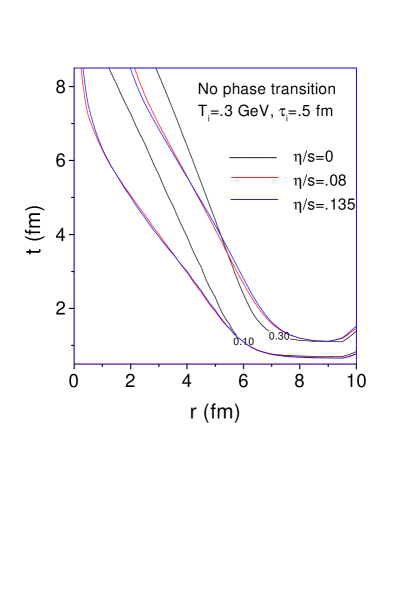
Figure 6: Contours of constant radial velocity in the $r{-}\tau$ plane for ideal and non-ideal hydrodynamic evolution, using $T_{i}$=0.3 GeV at $\tau_{i}$=0.5 fm/$c$.

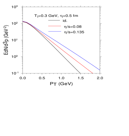
Figure 7: The final parton $p_{T}$ distribution at freeze-out ($T_{f}{\,=\,}160$ MeV). Initial temperature and time are $T_{i}{\,=\,}0.5$ GeV and $\tau_{i}{\,=\,}0.1$ fm/$c$.

4.2 Viscous corrections to the distribution function

The changed space-time evolution of the dissipative QGP may have significant effects on particle production. Although we cannot compute the $p_{T}$ spectra of final hadrons, since we did not include the hadronization phase transition, we can calculate the $p_{T}$ spectra of partons on the $T{\,=\,}T_{f}$ freeze-out surface.

When viscous corrections are included, the distribution function is modified from its local thermal equilibrium form [6, 11, 13]. When the viscous corrections are small, the distribution function can be written as

$$f(x,p)=f_{\rm eq}(x,p)(1+\Delta f)$$ (14)

with the equilibrium distribution function

$$f_{\rm eq}(x,p)=\frac{g}{2\pi^{2}}\frac{1}{e^{u\cdot p/T}\pm 1}\approx\frac{g}{2\pi^{2}}e^{-u\cdot p/T}.$$

If $\Delta f$ is restricted to 2nd order in $p^{\mu}$, its form can be determined as [6, 11, 13]

$$\Delta f=Cp_{\mu}p_{\nu}\pi^{\mu\nu}$$ (15)

where $C=\frac{1}{2(\varepsilon+p)T^{2}}$.

In Fig. 7, we show the parton $p_{T}$ spectra at $T_{f}{\,=\,}160$ MeV. The black line is for the ideal fluid. The red and blue lines are for non-ideal fluids with $\eta/s$=0.08 and 0.135, respectively. Viscous flow is seen to enhance high $p_{T}$ production by a factor 5–10, depending on viscosity. However, since $\pi^{\mu\nu}\neq 0$ already at initial time $\tau_{i}$, already the initial $p_{T}$ spectra for the viscous fluids are flatter than for the ideal fluid. To obtain the same measured final $p_{T}$-spectrum in the viscous case thus requires a retuning of initial conditions. This is presently under investigation.

5 Summary and conclusions

We have studied the effects of shear viscosity on the space-time evolution of a relativistic QGP fluid. In the 2nd order theory of dissipative fluid dynamics, the dissipative fluxes are treated as thermodynamic variables which follow kinetic relaxation equations. These are solved simultaneously with the energy-momentum conservation equations. Viscosity opposes expansion and cooling. Consequently, for a fixed freeze-out temperature, the freeze-out time (fluid lifetime) is increased. The evolution of the radial flow velocity is also changed – the viscous fluid generates more transverse flow. Viscous effects flatten the $p_{T}$ distribution and require a retuning of the initial conditions if the final spectra are to be kept fixed at their measured values.

Acknowledgement: The work of U.H. was supported by the U.S. Department of Energy under contract DE-FG02-01ER41190.

References

Appendix A Coordinate transformations

Instead of Cartesian coordinates $x^{\mu}=(t,x,y,z)$ we use curvilinear cylindrical coordinates in longitudinal proper time and rapidity, $\bar{x}^{m}=(\tau,r,\phi,\eta)$:

$$t = \tau\cosh\eta;\hskip 45.52458pt\tau=\sqrt{t^{2}-z^{2}}$$ (16)

$$x = r\cos\phi;\hskip 45.52458ptr=\sqrt{x^{2}+y^{2}}$$ (17)

$$y = r\sin\phi;\hskip 45.52458pt\phi=\tan^{-1}\left(\frac{y}{x}\right)$$ (18)

$$z = \tau\sinh\eta;\hskip 45.52458pt\eta=\frac{1}{2}\ln\frac{t+z}{t-z}.$$ (19)

The differentials

$$dt = d\tau\cosh\eta+d\eta\,\tau\sinh\eta,$$ (20)

$$dx = dr\,\cos\phi-d\phi\,r\sin\phi,$$ (21)

$$dy = dr\,\sin\phi+d\phi\,r\cos\phi,$$ (22)

$$dz = d\tau\sinh\eta+d\eta\,\tau\cosh\eta,$$ (23)

and the metric tensor is easily read off from

$$ds^{2} = g_{\mu\nu}dx^{\mu}dx^{\nu}=dt^{2}-dx^{2}-dy^{2}-dz^{2}$$ (24)

$$= \bar{g}_{mn}d\bar{x}^{m}d\bar{x}^{n}=d\tau^{2}-dr^{2}-r^{2}d\phi^{2}-\tau^{2}d\eta^{2},$$

namely

$$\bar{g}_{mn}=\left(\begin{array}[]{cccc}1&0&0&0\\ 0&-1&0&0\\ 0&0&-r^{2}&0\\ 0&0&0&-\tau^{2}\\ \end{array}\right),\hskip 28.45274pt\bar{g}^{mn}=\left(\begin{array}[]{cccc}1&0&0&0\\ 0&-1&0&0\\ 0&0&-1/r^{2}&0\\ 0&0&0&-1/\tau^{2}\\ \end{array}\right)$$ (25)

In curvilinear coordinates we must replace the partial derivatives with respect to $x^{\mu}$ by covariant derivatives (denoted by a semicolon) with respect to $\bar{x}^{m}$:

$${\bar{T}^{ik}}_{;p} = \frac{\partial\bar{T}^{ik}}{\partial\bar{x}^{p}}+\Gamma^{i}_{pm}\bar{T}^{mk}+\bar{T}^{im}\Gamma^{k}_{mp}.$$

The only non-vanishing Christoffel symbols are

$$\Gamma^{\tau}_{\eta\eta}=\tau;\quad\Gamma^{\eta}_{\tau\eta}=\Gamma^{\eta}_{\eta\tau}=1/\tau;\quad\Gamma^{r}_{\phi\phi}=-r;\quad\Gamma^{\phi}_{r\phi}=\Gamma^{\phi}_{\phi r}=1/r.$$ (26)

The hydrodynamic 4-velocity $u^{\mu}=\gamma(1,v_{x},v_{y},v_{z})$ is transformed to $\bar{u}^{m}=\gamma(1,v_{r},0,0)$, with $\gamma=1/\sqrt{1{-}v^{2}_{r}}$. From here on, we drop the bars over tensor components in $\bar{x}$-coordinates for simplicity.

Appendix B Relaxation equations for the viscous pressure tensor

Being symmetric and traceless, the viscous pressure tensor $\pi^{\mu\nu}$ has 9 independent components. The assumption of boost invariance reduces this number by 3 ($\nabla^{\left\langle m\right.}u^{\left.\eta\right\rangle}{\,=\,}0,\ m\neq\eta$). The additional assumption of cylindrical symmetry eliminates two more components ($\nabla^{\left\langle m\right.}u^{\left.\phi\right\rangle}{\,=\,}0,\ \eta\neq{m}\neq\phi$. The transversality condition $u_{m}\pi^{mn}=0$ eliminates another two components ($u_{\phi}$ and $u_{\eta}$ vanish and thus yield no constraints). Thus, with boost-invariance and cylindrical symmetry, the viscous pressure tensor has only two independent components which we here choose as $\pi^{rr}$ and $\pi^{\phi\phi}$.

The viscous pressure tensor relaxes on a short kinetic time scale $\tau_{\pi}$ to $2\eta$ times the shear tensor $\sigma^{\mu\nu}=\nabla^{\left\langle\mu\right.}u^{\left.\nu\right\rangle}$ [6]. The relaxation equations for $\pi^{rr}$ and $\pi^{\phi\phi}$ are

$$\partial_{\tau}\pi^{rr}+v_{r}\partial_{r}\pi^{rr} = -\frac{1}{\tau_{\pi}\gamma}\left(\pi^{rr}-2\eta\nabla^{\left\langle r\right.}u^{\left.r\right\rangle}\right),$$ (27)

$$\partial_{\tau}\pi^{\phi\phi}+v_{r}\partial_{r}\pi^{\phi\phi} = -\frac{1}{\tau_{\pi}\gamma}\left(\pi^{\phi\phi}-2\eta\nabla^{\left\langle\mu\right.}u^{\left.\phi\right\rangle}\right).$$ (28)

The $(rr)$ and $(\phi\phi)$ components of the shear tensor can be written as

$$\nabla^{\left\langle r\right.}u^{\left.r\right\rangle} = -\partial_{r}u^{r}-u^{r}Du^{r}-\frac{1}{3}\Delta^{rr}\partial{\cdot}u=\gamma^{2}\left(\frac{\partial{\cdot}u}{3}-\partial_{\tau}\gamma-\partial_{r}(\gamma v_{r})\right),$$ (29)

$$\nabla^{\left\langle\phi\right.}u^{\left.\phi\right\rangle} = -\frac{1}{r^{2}}\frac{u^{r}}{r}-\frac{1}{3}\Delta^{\phi\phi}\partial{\cdot}u=\frac{1}{r^{2}}\left(\frac{\partial{\cdot}u}{3}-\frac{\gamma v_{r}}{r}\right),$$ (30)

with the scalar expansion rate

$$\partial{\cdot}u=\partial_{\tau}u^{\tau}+\partial_{r}u^{r}+\frac{u^{\tau}}{\tau}+\frac{u^{r}}{r}=\left(\partial_{\tau}+\frac{1}{\tau}\right)\gamma+\left(\partial_{r}+\frac{1}{r}\right)(\gamma v_{r})$$ (31)

and the convective detivative

$$D=u\cdot\partial=\gamma(\partial_{\tau}+v_{r}\partial_{r}).$$ (32)

The projectors $\Delta^{rr}$ and $\Delta^{\phi\phi}$ are,

$$\Delta^{rr} =g^{rr}-u^{r}u^{r}=-1-(u^{r})^{2}=-\gamma^{2}$$

$$\Delta^{\phi\phi} =g^{\phi\phi}-u^{\phi}u^{\phi}=-\frac{1}{r^{2}}.$$

The remaining non-vanishing components of the viscous pressure tensor $\pi^{\tau\tau}$, $\pi^{\tau r}$, and $\pi^{\eta\eta}$ are eliminated using the constraints $u_{m}\pi^{mn}=0$ and $g_{mn}\pi^{mn}=0$, yielding

$$\pi^{\tau\tau}=v_{r}\pi^{\tau r}=v^{2}_{r}\pi^{rr},\quad\pi^{\eta\eta}=-\frac{1}{\tau^{2}}\left(-\frac{\pi^{rr}}{\gamma^{2}}+r^{2}\pi^{\phi\phi}\right).$$ (33)

Appendix C Energy-momentum conservation

With longitudinal boost-invariance and cylindrical symmetry, the energy-momentum conservation equations ${T^{mn}}_{;n}=0$ yield

$$\partial_{\tau}\tilde{T}^{\tau\tau}+\partial_{r}\left(v_{s}\tilde{T}^{\tau\tau}\right) = -\frac{\tilde{p}-\tilde{\pi}^{rr}/\gamma^{2}-r^{2}\tilde{\pi}^{\phi\phi}}{\tau},$$ (34)

$$\partial_{\tau}\tilde{T}^{\tau r}+\partial_{r}\left(v_{r}\tilde{T}^{\tau r}\right) = \frac{\tilde{p}+r^{2}\pi^{\phi\phi}}{r}-\partial_{r}\left(\tilde{p}+\frac{\tilde{\pi}^{rr}}{\gamma^{2}}\right).$$ (35)

where $\tilde{A}^{mn}\equiv r\tau A^{mn}$, $\tilde{p}\equiv r\tau p$, and $v_{s}\equiv T^{\tau r}/T^{\tau\tau}$.

References

- [1] Karsch F, Laermann E, Petreczky P, Stickan S and Wetzorke I, 2001 Proccedings of NIC Symposium (Ed. H. Rollnik and D. Wolf, John von Neumann Institute for Computing, Jülich, NIC Series, vol.9, ISBN 3-00-009055-X, pp.173-82,2002.)
- [2] see 2004 Proccedings of 17th International Conference on Ultra Relativistic Nucleus-Nucleus Collisions (Quark Matter 2004), Oakland, California, 11-17 Jan 2004. Published in 2004 J. Phys. G 30
- [3] Kolb P E and Heinz U Preprint nucl-th/0305084
- [4] Eckart C 1940 Phys. Rev. 58 919
- [5] Landau L D and Lifshitz E M 1959 Fluid Mechanics (Pergamon, MewYork)
- [6] Grad H, 1949 Commun. Pure Appl. Math. 2 331; Mueller I 1967 Z. Phys. 198 329; Israel W 1976 Ann. Phys. (N.Y.) 100 310; Stewart J M 1977 Proc. Roy. Soc. A 357 59; Israel W and Stewart J M 1979 Ann. Phys. (N.Y.) 118 341
- [7] Kajantie K 1984 Nucl. Phys. A 418 41c; Baym G 1984 Nucl. Phys. A 418 525c; Hosoya A and Kajantie K 1985 Nucl. Phys. B 250 666
- [8] Danielewicz P and Gyulassy M 1985 Phys. Rev. D bf 31 666
- [9] Chaudhuri A K 1995 Phys.Rev. Cbf 512889, 2000 J. Phys. G 26 1433, 2000 Phys. Scripta 61 311
- [10] Muronga A 2004 Phys. Rev. C 69 044901 (Preprint nucl-th/0309055)
- [11] Teaney D 2003 Phys. Rev. C 68 033913
- [12] Teaney D 2004 J. Phys. G: Nucl. Part. Phys. 30 S1247
- [13] Muronga A and Rischke D H Preprint nucl-th/0407114
- [14] Boris J P and Book D L 1976 Methods in computational Physics 16 85
- [15] Rischke D H, Bernard S and Maruhn J A 1995 Nucl. Phys.A 595 346
- [16] Baym G, Monien H, Pethick C J and Ravenhall D G 1990 Phys. Rev. Lett 64 1867
- [17] Arnold P, Moore G D and Yaffe L G 2000 J. High Energy. Phys. 0011 001 (for a complete leading order calculation see P. Arnold, G. D. Moore and L. G. Yaffe, 2003 J. High Energy. Phys. 0305 051)
- [18] Policastro G, Son D T and Starinets A O 2001 Phys. Rev. Lett.87 081601; 2002 J. High Energy Phys. 09 043 (Preprint hep-th/0210220)