Abstract

Hyperfine intervals in light hydrogenic atoms and ions are among the most accurately measured quantities in physics. The theory of QED corrections has recently advanced to the point that uncalculated terms for hydrogenic atoms and ions are probably smaller than 0.1 parts per million (ppm), and the experiments are even more accurate. The difference of the experiments and QED theory is interpreted as the effect on the hyperfine interaction of the (finite) nuclear charge and magnetization distributions, and this difference varies from tens to hundreds of ppm. We have calculated the dominant component of the 1s hyperfine interval for deuterium, tritium and singly ionized helium, using modern second-generation potentials to compute the nuclear component of the hyperfine splitting for the deuteron and the trinucleon systems. The calculated nuclear corrections are within 3% of the experimental values for deuterium and tritium, but are about 20% discrepant for singly ionized helium. The nuclear corrections for the trinucleon systems can be qualitatively understood by invoking SU(4) symmetry.

1 Introduction

The physics of hyperfine structure (hfs) is driven by magnetic interactions. This physics has a short-range nature, and is more complicated and challenging than “softer” regimes in atomic physics. This is especially true of the nuclear contribution to hyperfine structure, because the nuclear current density is more complicated than the nuclear charge density and less well understood[1, 2].

Until very recently hyperfine splittings in light hydrogenic atoms were by far the most precisely measured atomic transitions. Many of these very accurate experiments date back nearly half a century. Theoretical predictions are far less accurate, but have improved considerably in recent years. Non-recoil and non-nuclear contributions[3, 4] are known through order $\alpha^{3}E_{\rm F}$, where $E_{\rm F}$ is the Fermi hyperfine energy (viz., the leading-order contribution) and $\alpha$ is the fine-structure constant. Because the hadronic scales for recoil and certain types of nuclear corrections are the same, recoil corrections are treated on the same footing as nuclear corrections[3], and we will call both types “nuclear corrections.” It is very likely that the uncalculated QED terms of order $\alpha^{4}E_{\rm F}$ in light atoms contribute less than 0.1 ppm. Although much larger than the experimental errors, this is still significantly smaller than the nuclear corrections. We restrict ourselves to hydrogenic s-states in this work, because these states maximize nuclear effects.

Table I. $n^{3}(E_{\rm hfs}^{\rm exp}-E_{\rm hfs}^{\rm QED})/E_{\rm F}\,{\rm(ppm)}$ State H ²H ³H ³He⁺ 1s $-$33 138 $-$38 $-$212 2s $-$33 137 $--$ $-$211

Table 1: Difference between hyperfine experiments and QED hyperfine calculations for the $n\underline{\rm th}$ s-state of light hydrogenic atoms times $n^{3}$, expressed as parts per million of the Fermi energy. This difference is interpreted as nuclear contributions to the hyperfine splitting[4]. A negative entry indicates that the theoretical prediction without nuclear corrections is too large

Table I is an updated version of the corresponding table in Ref.[4]. Because hyperfine splittings are dominated by short-range physics, we expect the splittings in the $n\underline{th}$ s-state to be proportional to $|\phi_{n}(0)|^{2}\sim 1/n^{3}$, where $\phi_{n}(r)$ is the non-relativistic wave function of the electron. Forming the fractional differences (in parts per million) between $E^{\rm exp}_{\rm hfs}$ and $E^{\rm QED}_{\rm hfs}$ leads to the tabulated results. These large differences reflect neither experimental errors nor uncertainties in the QED calculations; they directly reflect large nuclear contributions.

One complication in performing the nuclear calculation is obtaining a final result that is tractable for numerical calculations. A framework fortunately exists for performing systematic expansions[2] of nuclear matrix elements in powers of $(Q/\Lambda)$, where $Q$ is a typical nuclear momentum scale that can be taken to be roughly the pion mass ($m_{\pi}\sim$ 140 MeV), and $\Lambda$ is the large-mass QCD scale ($\sim$ 1 GeV) typical of QCD bound states such as the nucleon, heavy mesons, nucleon resonances, etc. This framework, called power counting, also extends to nuclei, where $1/Q$ specifies a typical correlation length (and a reasonable nearest-neighbor distance) in light nuclei ($\sim$ 1.4 fm). This expansion in powers of $(Q/\Lambda\sim 0.1-0.15)$ should converge moderately well. For the purposes of this initial work, we restrict ourselves to leading-order terms in the nuclear corrections.

This restriction eliminates nuclear corrections of relativistic order, which we will briefly discuss later. There have been relatively few relativistic calculations in light nuclei because of the complexity of the nuclear force. The calculations that exist are known to generate rather small corrections[5], and they are especially small in the deuteron case because of its weak binding[6]. Few calculations exist for the much more complicated three-nucleon systems[7]. Most nuclear physics knowledge and lore in light nuclei is non-relativistic in nature.

In processes that involve virtual excitation of intermediate nuclear states (each state $|N\rangle$ with its own energy, $E_{N}$, relative to the ground-state energy, $E_{0}$) the excitation energy $(\omega_{N}=E_{N}-E_{0})$ is of order $Q^{2}/\Lambda$ and typically is a correction to the leading order[2]. Consistency therefore demands that we drop such terms. The nuclear recoil energy $Q^{2}/2M$, where $M$ is the nuclear mass, has the same scale and can also be dropped.

Our goal is to evaluate the deuteron contribution in leading order as carefully as possible, and to use the impulse approximation to evaluate the ³He and ³H results. This restriction should be accurate to within the 10-15% uncertainty of our leading-order approximation and adequate for a first calculation of the trinucleon sector. This level of accuracy does require the inclusion of the intrinsic hyperfine structure of the nucleons. We will see that the calculated results are good for deuterium and tritium and fairly good for ³He⁺. Our goal is to present a simple and compelling picture of the nuclear hyperfine structure in $d$, ³H, and ³He⁺, using a unified approach for all. To accomplish this we invoke a simple and intuitive model of trinucleon structure based on SU(4) symmetry that is sufficiently accurate to explain the patterns in Table I.

2 Nuclear Contributions to Hyperfine Structure

The hyperfine interactions that interest us are simple (effective) couplings of the electron spin to the nuclear (ground-state) spin: $\vec{\sigma}\cdot\vec{S}$ where $\vec{\sigma}$ is the electron (Pauli) spin operator and $\vec{S}$ is the nuclear spin (i.e., the total angular momentum[8]) operator. Other couplings of the electron spin are possible and either generate no hyperfine splitting, none in s-states, or higher-order (in $\alpha$) contributions. Coupling of the electron spin to the electron angular momentum (i.e., the electron spin-orbit interaction, which vanishes in s-states) is one example.

We begin with a sketch of the Fermi hyperfine splitting in order to establish our notation and conventions. The electron charge operator ($\psi^{\dagger}\psi$) is a space scalar, and by itself does not generate a term of the desired form because nuclear-spin information cannot be transmitted via the exchange of the appropriate component of the virtual photon’s propagator. The leading-order term in the hyperfine energy shift consequently has the (usual) form of a current-current interaction.

$$E_{\rm F}=\alpha\,\int d^{3}r\int d^{3}r^{\prime}\,\frac{\psi^{\dagger}(\vec{\,r})\vec{\alpha}\,\psi(\vec{\,r})\,\cdot\vec{J}(\vec{\,r}^{\prime})}{|\vec{\,r}-\vec{\,r}^{\prime}|}\,,$$

where $\psi^{\dagger}\vec{\alpha}\psi$ is the current density of the (Dirac) electron and $\vec{J}(\vec{\,r}^{\prime})$ is the nuclear (ground-state) current density. Ignoring higher-order (in $\alpha$) terms this expression can be manipulated into the form

$$E_{\rm F}=\frac{\alpha}{2m_{e}}\int d^{3}r\;|\phi_{n}(r)|^{2}\int d^{3}r^{\prime}\,\vec{J}(\vec{\,r}^{\prime})\cdot\vec{\sigma}\times\vec{\nabla}_{r}\frac{1}{|\vec{\,r}-\vec{\,r}^{\prime}|}\,,$$

where $m_{e}$ is the electron mass and $\phi_{n}(r)$ is the usual non-relativistic atomic $n\underline{\rm th}$ s-state wave function. The restriction to atomic s-states limits the current to the magnetic-dipole part, which can be written in terms of the magnetic-dipole operator, $\vec{\mu}$, as

$$\vec{J}(\vec{\,r})\rightarrow\vec{J}_{M1}(\vec{\,r})=\vec{\nabla}_{r}\times\vec{\mu}(\vec{\,r})\,,$$

and $\vec{\mu}$ can be written in terms of the nuclear ground-state magnetization density $\rho_{M}(r)$ as

$$\vec{\mu}(\vec{\,r})=\frac{\mu^{\phantom{|}}_{N}\,\vec{S}}{S}\,\rho_{M}(r)\,,$$

where $\int d^{3}\,r^{\prime}\rho_{M}(r^{\prime})=1$ and $\langle SS|\mu_{\rm z}|SS\rangle\equiv\mu^{\phantom{|}}_{N}$ defines the nuclear magnetic moment. We finally obtain the Fermi hyperfine energy in the limit $\rho_{M}(r^{\prime})\rightarrow\delta^{3}(\vec{\,r}^{\prime})$:

$$E_{\rm F}=\frac{4\pi\alpha\mu^{\phantom{|}}_{N}}{3m_{e}}\frac{\vec{\sigma}\cdot\vec{S}}{S}\int d^{3}r|\phi_{n}(r)|^{2}\rho_{M}(r)=\frac{4\pi\alpha\mu^{\phantom{|}}_{N}|\phi_{n}(0)|^{2}}{3m_{e}}\frac{\vec{\sigma}\cdot\vec{S}}{S}\,,$$

where the factor of $(\vec{\sigma}\cdot\vec{S})/S$ leads to a hyperfine splitting of $(2\,S+1)/S$. All additional contributions will be measured as a fraction of this energy. We note that using the point-like $\rho_{M}$ and Eqn. (3a) in Eqn. (1) leads to an atomic matrix element $\int_{0}^{\infty}drF(r)G(r)$ (in the standard Dirac notation) that can be evaluated analytically for higher-order Coulomb corrections[3] to the leading contribution of ${\cal O}(Z^{3}\alpha^{4})$, where $Z$ is the nuclear charge. Note that $E_{\rm F}$ is independent of nuclear structure.

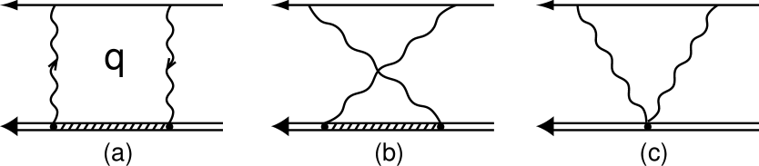
Figure 1: Nuclear Compton amplitude with direct (a), crossed (b), and seagull (c) contributions illustrated. Single lines represent an electron, double lines a nucleus, wiggly lines a photon propagator (with four-momentum $q^{\mu}$), and shaded double lines depict a nuclear Green’s function containing a sum over nuclear states. The seagull vertex maintains gauge invariance.

Naively calculating higher-order (in $\alpha$) corrections from the first part of Eqn. (4) fails because only that part of $\phi_{n}(r)$ inside the nucleus (i.e., within the magnetic “size”, $R_{M}$) contributes to the integral, and that is the (only) part of the electron’s wave function significantly modified by the nuclear charge distribution, $\rho_{\rm ch}(r)$, whose radius, $R_{\rm ch}$, is nearly the same as $R_{M}$. In other words a proper calculation[9, 10] must take into account modifications of $\phi_{n}(r)$ by $\rho_{\rm ch}$, and that necessarily involves one order in $\alpha$ higher than $E_{\rm F}$. Thus we need to perform a consistent second-order (in $\alpha$) calculation of the electron-nucleus interaction, depicted in Fig. (1).

These graphs are constructed from the direct, crossed, and nuclear seagull contributions to the nuclear Compton amplitude. Only the forward-scattering part of this amplitude is required for the ${\cal O}(\alpha)$ corrections to $E_{\rm F}$, and this generates a short-range atomic operator that samples the (upper-component) s-state wave functions only near the origin. The resulting energy shift is then given by

$$\Delta E=i(4\pi\alpha)^{2}|\phi_{n}(0)|^{2}\int\frac{d^{4}q}{(2\pi)^{4}}\frac{t_{\mu\nu}(q)\,T^{\mu\nu}(q,-q)}{(q^{2}+i\epsilon)^{2}(q^{2}-2m_{e}q_{0}+i\epsilon)}\,,$$

where $t^{\mu\nu}$ is the lepton Compton amplitude and $T^{\mu\nu}$ is the corresponding nuclear Compton tensor, both of which are required to be gauge invariant. The lepton tensor can be decomposed into an irreducible spinor basis; we can ignore odd matrices and spin-independent components, since they do not contribute to the hyperfine structure at ${\cal O}(\alpha E_{\rm F})$. We also ignore (with one exception treated later) terms that couple two currents together. It is easy to show that since the nuclear current scales as $1/\Lambda$ (the conventional components of the current have explicit factors of $1/M$), two of them should scale as $1/\Lambda^{2}$ and generate higher-order (in $1/\Lambda$) terms. This leaves a single term representing a charge-current correlation

$$\Delta E=(4\pi\alpha)^{2}|\phi_{n}(0)|^{2}\int\frac{d^{4}q}{(2\pi)^{4}}\frac{(\vec{\sigma}\times\vec{\,q})^{m}[T^{m0}(q,-q)-T^{0m}(q,-q)]}{(q^{2}+i\epsilon)^{2}(q^{2}-2m_{e}q_{0}+i\epsilon)}\,.$$

The seagull terms $B^{0m}(q,-q)$ and $B^{m0}(q,-q)$ are of relativistic order[11] $(\sim 1/\Lambda^{2})$ and can be dropped. Although the term $B^{mn}(\vec{\,q},-\vec{\,q})$ is of non-relativistic order, it does not contribute in conventional approaches because of crossing symmetry.

The explicit form for $T^{m0}$ (suppressing the nuclear ground-state expectation value, but including all intermediate states, $N$) is

$$T^{m0}(q,-q)=\sum_{N}\left(\frac{\,J^{m}(-\vec{\,q})\,|N\rangle\langle N|\,\rho(\vec{\,q})}{q_{0}-\omega_{N}+i\epsilon}+\frac{\,\rho(\vec{\,q})\,|N\rangle\langle N|\,J^{m}(-\vec{\,q})}{-q_{0}-\omega_{N}+i\epsilon}\right)\,,$$

which greatly simplifies Eqn. (6) in the limit $\omega_{N}\rightarrow 0$ and $m_{e}\rightarrow 0$, leading finally in this limit to a very simple form when closure is used

$$\Delta E=i(4\pi\alpha)^{2}|\phi_{n}(0)|^{2}\int\frac{d^{3}q}{(2\pi)^{3}}\frac{(\vec{\sigma}\times\vec{\,q})^{m}\{J^{m}(-\vec{\,q}),\rho(\vec{\,q})\}}{\vec{\,q}^{6}}\,,$$

which is infrared divergent. Using

$$J^{m}(-\vec{\,q})=\int d^{3}y\,J^{m}(\vec{y})e^{-i\vec{\,q}\cdot\vec{y}}\,,$$

and

$$\rho(\vec{\,q})=\int d^{3}x\,\rho(\vec{x})e^{i\vec{\,q}\cdot\vec{x}}\,,$$

together with $\vec{z}\equiv\vec{x}-\vec{y}$, and a lower-limit (infrared) $q-$cutoff, $\epsilon$, we find

$$\Delta E=-8\alpha^{2}|\phi_{n}(0)|^{2}\int d^{3}x\int d^{3}y\,\{\rho(\vec{x}),\vec{\sigma}\cdot\vec{J}(\vec{y})\}\times\vec{\nabla}_{\rm z}\left(\frac{1}{3\epsilon^{3}}-\frac{z^{2}}{6\epsilon}+\frac{\pi z^{3}}{48}\right)\,,$$

where there is an implied (nuclear) expectation value. The constant term does not contribute because of the derivative, the $z^{2}$-term contributes a term proportional to $\frac{-(\vec{x}-\vec{y})}{3\epsilon}$, and the last term is the term we are seeking.

The remaining singular (second) term must be treated more carefully. The part proportional to $\vec{y}$ leads (because of the integral over $\vec{x}$) to a contribution proportional to $Z$, the total nuclear charge, and $\mu^{\phantom{|}}_{N}$, the nuclear magnetic moment. Since this contribution is already part of $E_{\rm F}$, keeping this term would amount to double counting, and we therefore ignore it. The $\vec{x}$-term on the other hand generates (unretarded) dipole transitions, and the singularity $(1/\epsilon)$ arises from neglecting $1/\omega_{N}$ and $m_{e}$ terms. Siegert’s theorem[1] for unretarded electric dipole transitions ($\int d^{3}y\vec{J}(\vec{y})\sim i\omega_{N}\vec{D}$) generates an additional factor of $\omega_{N}$ (i.e., $\epsilon$) so this singular term is actually of the form $(\epsilon/\epsilon)\rightarrow(0/0)$ and requires a careful calculation. A rather tedious evaluation of this term in Eqn. (6) leads to $\Delta E_{a}=-2i\alpha^{2}|\phi_{n}(0)|^{2}\vec{\sigma}\cdot\vec{D}$ $(\ln\frac{2(H-E_{0})}{m_{e}}+3/2)\times\vec{D}$ where $H-E_{0}\equiv\omega_{N}$ in intermediate states. A similar term arises in the product of two currents mentioned above Eqn. (6) and leads to $\Delta E_{b}=-i\alpha^{2}|\phi_{n}(0)|^{2}\vec{\sigma}\cdot\vec{D}$ $(\ln\frac{2(H-E_{0})}{m_{e}}-1/2)\times\vec{D}$.

These contributions are completely unimportant, as we now demonstrate. The constant terms (including $\ln(m_{e})$) are proportional to $\vec{\sigma}\cdot\vec{D}\times\vec{D}$, which vanishes for non-relativistic dipole operators because they commute. Replacing $\omega_{N}$ by a constant (viz., the closure approximation) similarly vanishes. It is straightforward to show that the nuclear matrix element also vanishes in zero-range approximation, where one neglects the deuteron d-state and the potential in intermediate states (the structure of the dipole operator weights the tails of the wave functions, and this minimizes the effect of the intermediate-state nuclear potential). In perturbation theory it is possible to show that only the spin-orbit combination of potentials in intermediate states contributes (i.e., central and tensor terms cancel), and this small potential is of relativistic order $(1/\Lambda^{2})$, which we have previously agreed to ignore. One can also show that the non-vanishing deuteron contribution is proportional to $\eta^{2}$, the square of the d- to s-wave asymptotic normalization constant $(\sim(0.025)^{2})$, which is extremely small. A recent brute-force numerical calculation confirms these estimates[12]. The terms $\Delta E_{a}$ and $\Delta E_{b}$ are therefore numerically negligible and can be ignored.

Our final result in leading order is a relatively simple expression originally developed in a limiting case by Low[13] for the deuteron, as sketched by Bohr[14] for the same system:

$$\Delta E^{\rm Low}_{\rm hfs}=\frac{\pi\alpha^{2}|\phi_{n}(0)|^{2}}{2}\int d^{3}x\int d^{3}y\,\{\rho(\vec{x}),\vec{\sigma}\cdot\vec{z}\times\vec{J}(\vec{y})\}\,z+\cdots\,,$$

where both an atomic and nuclear expectation value is implied, but has been ignored in Eqn. (11a) and subsequent equations for reasons of simplicity.

A more convenient representation of this result is obtained by dividing both sides by the expression for the Fermi hyperfine energy given by Eqn. (4). Since the Wigner-Eckart Theorem guarantees that the resulting form of Eqn. (11a) must be proportional to $\vec{\sigma}\cdot\vec{S}/S$ (which cancels in the ratio), we arrive at a simple but powerful expression for the leading-order contribution:

$$\Delta E^{\rm Low}_{\rm hfs}=-2m_{e}\,\alpha\,\delta_{\rm Low}\,,$$

where

$$\delta_{\rm Low}=-\frac{3}{16\mu^{\phantom{|}}_{N}}\int d^{3}x\int d^{3}y\,\{\rho(\vec{x}),(\vec{z}\times\vec{J}(\vec{y}))_{\rm z}\}|\vec{x}-\vec{y}|\,,$$

and an expectation value is required of the z (or “3”) component of the vector $\vec{z}\times\vec{J}(\vec{y})$ in the nuclear state with maximum azimuthal spin (i.e. $S_{\rm z}=S$). The intrinsic size of the nuclear corrections is given by ($-2\,m_{e}\,\alpha R$) = $-$38 ppm $[R/$fm], where $[R/$fm] is the value of the Low moment in Eqn. (11c) in units of fm. The results of Table I therefore suggest (correctly) that Low moments are on the order of a few fermi in light nuclei, which is quite sensible.

3 Nuclear Matrix Elements

We predicate our discussion with the deuteron in mind. Other nuclei can and will be treated mutatis mutandis. The isospin of the deuteron ($T=0$) makes it a useful first case. We note that the nuclear physics in Eqn. (11) involves the correlation between the nuclear charge operator, $\rho(\vec{x})$, and the nuclear current operator, $\vec{J}(\vec{y})$. If one inserts a complete set of states between these operators, there will be both elastic contributions (i.e., ground-state expectation values) that are called Zemach corrections[10], and inelastic contributions (called nuclear polarization corrections). Although we will calculate (or estimate) both types, it is much easier to calculate the sum of the two.

The nuclear charge operator contains both isoscalar and isovector pieces, and is non-relativistic in leading order. We ignore relativistic corrections, as we discussed earlier. We therefore write the charge operator in the form

$$\rho(\vec{x})=\sum_{i=1}^{A}\hat{e}_{i}(|\vec{x}-\vec{x}^{\prime}_{i}|)\,,$$

where

$$\hat{e}_{i}(|\vec{x}-\vec{x}^{\prime}_{i}|)=\hat{p}_{i}\,\rho^{p}_{ch}(|\vec{x}-\vec{x}^{\prime}_{i}|)+\hat{n}_{i}\,\rho^{n}_{ch}(|\vec{x}-\vec{x}^{\prime}_{i}|)\,,$$

and

$$\hat{p}_{i}=\left(\frac{1+\tau^{3}_{i}}{2}\right)\,,$$

and

$$\hat{n}_{i}=\left(\frac{1-\tau^{3}_{i}}{2}\right)\,.$$

This decomposes the i$\underline{th}$ nucleon’s charge operator into proton plus neutron parts. The densities $\rho^{p}_{ch}$ and $\rho^{n}_{ch}$ are the intrinsic charge densities of the proton and neutron, respectively, while $\hat{p}_{i}$ and $\hat{n}_{i}$ are the proton and neutron isotopic projection operators, respectively. The coordinate $\vec{x}^{\prime}_{i}$ is the distance of the i$\underline{th}$ nucleon from the nuclear center of mass. We expect that the neutron charge density should play a very minor role, and we will find (later) that its contribution is only a few percent of that of the proton. Rather sophisticated models exist for the Fourier transform (i.e., the form factor) of $\rho^{p}_{ch}$[17].

The nuclear current operator is more complicated, even if we ignore relativistic corrections (which we will). The problem is the mechanism underlying the nuclear force (viz., the exchange of charged mesons), which can also contribute to the nuclear current in the form of meson-exchange currents (MEC). These currents largely vanish for isoscalar transitions (such as the deuteron ground state) because there is no net flow of charge, but they can be sizable (10% - 20%) for isovector transitions. One can show that their contribution to the deuteron in Eqn. (11) almost entirely vanishes, and we will henceforth ignore these currents below Eqn. (13). We formally expand the current into convection, spin-magnetization, and meson-exchange parts

$$\vec{J}(\vec{y})=\vec{J}_{C}(\vec{y})+\vec{\nabla}_{y}\times\vec{\mu}(\vec{y})+\vec{J}_{\rm MEC}(\vec{y})+\cdots\,,$$

where

$$\vec{J}_{C}(\vec{y})=\sum_{i=1}^{A}\left\{\frac{\vec{\pi}_{i}}{2M},\hat{e}_{i}(|\vec{y}-\vec{x}^{\prime}_{i}|)\right\}\,$$

is the nuclear convection current, $\vec{\pi}_{i}$ is the i$\underline{th}$ nucleon’s momentum in the nuclear center-of-mass frame,

$$\vec{\mu}(\vec{y})=\sum_{i=1}^{A}\vec{\sigma}_{i}\,\hat{\mu}_{i}(|\vec{y}-\vec{x}^{\prime}_{i}|)\,$$

is the impulse-approximation magnetic-moment operator, $\vec{J}_{\rm MEC}$ is the nuclear meson-exchange current, and

$$\hat{\mu}_{i}(|\vec{y}-\vec{x}^{\prime}_{i}|)=\hat{p}_{i}\,\mu^{\phantom{|}}_{p}\,\rho^{p}_{M}(|\vec{y}-\vec{x}^{\prime}_{i}|)+\hat{n}_{i}\,\mu^{\phantom{|}}_{n}\,\rho^{n}_{M}(|\vec{y}-\vec{x}^{\prime}_{i}|)\,$$

is the nucleon magnetization density for the ith nucleon expressed in terms of protons and neutrons separately. The quantities $\mu^{\phantom{|}}_{p}$ and $\mu^{\phantom{|}}_{n}$ are the (total) proton and neutron magnetic moments, while $\rho^{p}_{M}$ and $\rho^{n}_{M}$ are the intrinsic proton and neutron magnetization densities (normalized to 1).

Using Eqns. (12) and (13) the energy shift in Eqns. (11) can be evaluated. Rather than split Eqn. (11c) into Zemach terms (by inserting intermediate ground states between $\rho$ and $\vec{J}$) and polarization terms (by inserting intermediate excited nuclear states between $\rho$ and $\vec{J}$), we will use the fact that our charge and current operators are each given by a sum over single-nucleon operators. Thus their product can be decomposed into single-nucleon plus two-nucleon operators. These forms are particularly convenient to evaluate. We first write in an obvious notation that

$$\delta_{\rm Low}=\delta_{\rm spin}^{(1)}+\delta_{\rm Low}^{(2)}\,.$$

Note that the quantity $\delta_{\rm spin}^{(1)}$ was not part of Low’s original work, nor was there any evidence at that time that such a term might be significant. We next use Eqns. (13) to manipulate the magnetization part of the current in Eqn. (11c) into the form (recall that $\vec{z}=\vec{x}-\vec{y}$)

$$\delta_{\rm Low}^{\rm mag}=\frac{1}{\mu^{\phantom{|}}_{N}}\sum_{i,j}^{A}\int d^{3}x\int d^{3}y\,|\vec{x}-\vec{y}|\,\hat{e}_{i}(|\vec{x}-\vec{x}^{\prime}_{i}|)\hat{\mu}_{j}(|\vec{y}-\vec{x}^{\prime}_{j}|)\left(\vec{\sigma}_{j}-\frac{1}{8}(3\vec{\sigma}_{j}\cdot\hat{z}\hat{z}-\vec{\sigma}_{j})\right)_{\rm z}\,,$$

while the convection current can be reduced to

$$\delta_{\rm Low}^{\rm conv}=-\frac{3}{16\mu^{\phantom{|}}_{N}M}\sum_{i,j}^{A}\int d^{3}x\int d^{3}y\,|\vec{x}-\vec{y}|\{(\vec{z}\times\vec{\pi}_{j})_{\rm z},\hat{e}_{i}(|\vec{x}-\vec{x}^{\prime}_{i}|)\hat{e}_{j}(|\vec{y}-\vec{x}^{\prime}_{j}|)\}\,.$$

The one-body $(i=j)$ part of the convection-current contribution vanishes upon integration, as does the second (tensor) term in the magnetization contribution. Shifting the variables $\vec{x}$ and $\vec{y}$ by $\vec{x}^{\prime}_{i}$ leads to

$$\delta_{\rm spin}^{(1)}=\sum_{i=1}^{A}\left(\langle r\rangle^{pp}_{(2)}\frac{\mu^{\phantom{|}}_{p}}{\mu^{\phantom{|}}_{N}}\,\hat{p}_{i}+\langle r\rangle^{nn}_{(2)}\frac{\mu^{\phantom{|}}_{n}}{\mu^{\phantom{|}}_{N}}\,\hat{n}_{i}\right)\sigma_{i}^{\rm z}\,,$$

where

$$\langle r\rangle^{pp}_{(2)}=\int d^{3}x\int d^{3}y\,\rho^{p}_{ch}(x)\rho^{p}_{M}(y)|\vec{x}-\vec{y}|=1.086(12){\,\rm fm}\,,$$

and

$$\langle r\rangle^{nn}_{(2)}=\int d^{3}x\int d^{3}y\,\rho^{n}_{ch}(x)\rho^{n}_{M}(y)|\vec{x}-\vec{y}|\,$$

determine the proton and neutron parts of the one-body current. Note that the quantities $\langle r\rangle^{pp}_{(2)}$ and $\langle r\rangle^{nn}_{(2)}$ are the usual proton and neutron Zemach terms, and we have listed in Eqn. (18a) the value of the proton Zemach moment recently determined directly from the electron-scattering data for the proton[15] (the neutron has not been evaluated). In numerical work described below we will use simple forms for the neutron and proton form factors: a dipole form for the proton charge and magnetic form factors and the neutron magnetic form factor $(F_{D}(q^{2})=\frac{1}{(1+q^{2}/\beta^{2})^{2}})$ and a modified Galster[16] form for the neutron charge form factor $(F_{G}=\frac{\lambda\,q^{2}}{(1+q^{2}/\beta^{2})^{3}})$. To incorporate into our calculations the numerical value given by Eqn. (18a) we use $\beta=4.0285$ fm^-1, which reproduces this value for the dipole case (see Appendix A for moments and correlation functions determined by this choice of form factors). The r.m.s. radius determined by this $\beta$ is 0.86 fm, which is slightly smaller than the proton charge radius[17] but slightly larger than its magnetic radius[18] and thus represents an average value. The much smaller neutron moment, $\langle r\rangle_{(2)}^{nn}$ (see Appendix A), can be adequately represented using this value of $\beta$ and $\lambda=0.0190$ fm², which determines the neutron charge radius[19]. These numbers lead to $\langle r\rangle_{(2)}^{nn}=-0.042$ fm, which we will use below. Because this value is such a small fraction of the proton result, the uncertainty in the neutron value plays no significant role.

Equation (17) is still a nuclear operator, and its expectation value depends on the nucleus. We begin with the deuteron (which has $T=0$) and this eliminates the $\tau_{3}$ terms in $\hat{p}_{i}$ and $\hat{n}_{i}$. The spin terms then sum to $(\vec{\sigma}_{1}+\vec{\sigma}_{2})_{\rm z}$, which is not the total angular momentum (it lacks $\vec{L}$, the orbital angular momentum contribution). The expectation value of $(\vec{\sigma}_{1}+\vec{\sigma}_{2})_{\rm z}$ is $2S_{\rm z}(1-\frac{3}{2}P_{D})$, where $S_{\rm z}$ is the z-component of the deuteron total angular momentum operator and $P_{D}$ is the amount of $D$-wave in the deuteron wave function (typically, slightly in excess of 5.6%). In the state of maximum $S_{\rm z}$ this leads to

$$\delta_{d}^{(1)}=(1-\frac{3}{2}P_{D})\left(\frac{\mu^{\phantom{|}}_{p}}{\mu^{\phantom{|}}_{d}}\langle r\rangle^{pp}_{(2)}+\frac{\mu^{\phantom{|}}_{n}}{\mu^{\phantom{|}}_{d}}\langle r\rangle^{nn}_{(2)}\right)\,,$$

which is completely dominated by the proton. Note that the $D$-wave prefers to anti-align with the spin, which leads to the reduction in Eqn. (19).

A similar (though more complicated) analysis is possible for ³He and ³H (see Appendix B). The traditional (and very useful) decomposition of the trinucleon wave function uses representations of spin-isospin symmetry (viz., SU(4)). In addition to the somewhat larger D-state component $(P_{D}\sim 9\%)$, the significant $S$-wave component comes in two distinct types: the dominant S-state ($P_{S}\sim 90\%$) with a completely antisymmetric spin-isospin wave function and completely symmetric space wave function, and the mixed-symmetry S^′-state $(P_{S^{\prime}}\sim 1\%)$. The representations of SU(4) were used long ago to decompose contributions to the trinucleon magnetic moments, and this leads to[20, 21]

$$\openup 3.0pt\halign to=0.0pt{\hfil$\displaystyle{#}$ &$\displaystyle{{}#}$\hfil&\llap{$#$}\cr\left\langle\sum_{i=1}^{A} \left( \frac{1 \pm\tau^{3}_{i}}{2} \right) \vec{\sigma}_{i} \right\rangle=&\vec{S}\left( (1-2 P_{D}) \mp\tau_{3} (1 - \frac{4}{3} P_{S^{\prime}} - \frac{2}{3} P_{D}) \right) \, , &\hbox to0.0pt{\hss$(20a)\cr=&2 \vec{S}\left\{ \left[ \begin{array}[]{c}\gamma\\ \xi\end{array} \right] \left( \frac{1+\tau_{3}}{2} \right) + \left[ \begin{array}[]{c}\xi\\ \gamma\end{array} \right] \left( \frac{1-\tau_{3}}{2} \right) \right\} \, , &\hbox to0.0pt{\hss$(20b)\cr}}}$$

where

$$\openup 3.0pt\halign to=0.0pt{\hfil$\displaystyle{#}$ &$\displaystyle{{}#}$\hfil&\llap{$#$}\cr\gamma&= \frac{2}{3} \left( P_{S^{\prime}} - P_{D} \right) \cong-0.06 \, , &\hbox to0.0pt{\hss$(21a)\cr\xi&= 1 - \frac{2}{3} P_{S^{\prime}} - \frac{4}{3} P_{D} \cong 0.86 \, , &\hbox to0.0pt{\hss$(21b)\cr}}}$$

specify the two sign cases in Eqns. (20a) and (20b). Note that $\tau_{3}$ is the third component of total isospin and $\vec{S}$ is the (total) nuclear-angular-momentum operator. The first and second terms in Eqn. (20b) determine ³He and ³H, respectively, while upper and lower components refer to $\pm$ in Eqn. (20a). Finally we obtain

$$\delta^{(1)}_{{}^{3}{\rm He}}=\frac{\mu^{\phantom{|}}_{p}\gamma}{\mu^{\phantom{.}}_{{}^{3}{\!\rm He}}}\langle r\rangle^{pp}_{(2)}+\frac{\mu^{\phantom{|}}_{n}\xi}{\mu^{\phantom{.}}_{{}^{3}{\!\rm He}}}\langle r\rangle^{nn}_{(2)}\rightarrow 0\,,$$

and

$$\delta^{(1)}_{{}^{3}{\rm H}}=\frac{\mu^{\phantom{|}}_{p}\xi}{\mu^{\phantom{.}}_{{}^{3}{\!\rm H}}}\langle r\rangle^{pp}_{(2)}+\frac{\mu^{\phantom{|}}_{n}\gamma}{\mu^{\phantom{.}}_{{}^{3}{\!\rm H}}}\langle r\rangle^{nn}_{(2)}\rightarrow\langle r\rangle^{pp}_{(2)}\,,$$

where the point-neutron, SU(4) symmetry limit (i.e., the S-state only, which is indicated by the arrow) is discussed below.

This result is very easy to interpret. In the dominant S-state (corresponding to $\gamma=0$ and $\xi=1$) the two “like” nucleons (e.g., the protons in ³He) have opposite and cancelling spins, while the “unlike” nucleon (e.g., the neutron in ³He) carries all of the spin and determines both the magnetic moment and the single-nucleon contribution to the hyperfine structure (if we ignore meson-exchange currents and the convection current). Ignoring those currents leads to $\mu^{\phantom{.}}_{{}^{3}{\!\rm He}}=\gamma\mu^{\phantom{|}}_{p}+\xi\mu^{\phantom{|}}_{n}\rightarrow\mu^{\phantom{|}}_{n}$ and $\mu^{\phantom{.}}_{{}^{3}{\!\rm H}}=\xi\mu^{\phantom{|}}_{p}+\gamma\mu^{\phantom{|}}_{n}\rightarrow\mu^{\phantom{|}}_{p}$, where the arrow indicates the SU(4) limit. The ³He single-nucleon contribution to hfs in this limit comes solely from the tiny neutron contribution, while the corresponding ³H contribution is simply $\langle r\rangle^{pp}_{(2)}$ and becomes identical to the free proton Zemach moment.

The two-nucleon contributions are more complicated and are determined by correlation functions. In the deuteron these correlations must be between a neutron and a proton and are of the types: $e_{p}-\mu^{\phantom{|}}_{n}$, $e_{n}-\mu^{\phantom{|}}_{p}$, and $e_{n}-e_{p}$ (convection current only). In the trinucleons there are additional types: $e_{p}-\mu^{\phantom{|}}_{p}$, $e_{n}-\mu^{\phantom{|}}_{n}$, and $e_{p}-e_{p}$ (convection current only). As we noted earlier the correlations involving $e_{n}$ will be very small, and we have ignored the tiny $e_{n}-e_{n}$ convection-current correlation in ³H.

The two-nucleon contributions contained in Eqns. (15) and (16) can be manipulated into simpler forms by shifting $\vec{x}$ by $\vec{x}^{\prime}_{i}$ and $\vec{y}$ by $\vec{x}^{\prime}_{j}$, leading to

$$\openup 3.0pt\halign to=0.0pt{\hfil$\displaystyle{#}$ &$\displaystyle{{}#}$\hfil&\llap{$#$}\cr\delta_{\rm Low}^{\rm mag} =&\frac{1}{\mu^{\phantom{|}}_{N}} \sum_{i \neq j}^{A} \left( \vec{\sigma}_{j} C_{i j} (x_{i j}) - \frac{1}{8} \bar{\! \bar{C}}_{i j} (x_{i j}) (3 \vec{\sigma}_{j} \cdot\hat{x}_{i j}\hat{x}_{i j}- \vec{\sigma}_{j})\right)_{\rm z} \, , &\hbox to0.0pt{\hss$(23a)\cr\delta_{\rm Low}^{\rm conv} =&\frac{3}{16 M \mu^{\phantom{|}}_{N}} \sum_{i \neq j}^{A} \bar{C}_{i j} (x_{i j}) L_{i j}^{\rm z} \, , &\hbox to0.0pt{\hss$(23b)\cr}}}$$

where $\vec{L}_{ij}=\vec{x}_{ij}\times(\vec{\pi}_{i}-\vec{\pi}_{j})$ and the three correlation functions are defined by

$$\openup 3.0pt\halign to=0.0pt{\hfil$\displaystyle{#}$ &$\displaystyle{{}#}$\hfil&\llap{$#$}\cr C_{i j} (r)&= \int d^{3} x \int d^{3} y \, \hat{e}_{i} (x) \hat{\mu}_{j} (y) |\vec{x}-\vec{y}+\vec{\, r}| \, , &\hbox to0.0pt{\hss$(24a)\cr&= \hat{p}_{i}(\mu^{\phantom{|}}_{p}\hat{p}_{j} + \mu^{\phantom{|}}_{n}\hat{n}_{j}) C_{DD} (r) + \hat{n}_{i}(\mu^{\phantom{|}}_{p}\hat{p}_{j} + \mu^{\phantom{|}}_{n}\hat{n}_{j}) C_{DG} (r) \, , &\hbox to0.0pt{\hss$(24b)\cr\bar{C}_{i j} (r)&= \frac{1}{3 r}\frac{d\;}{dr} \int d^{3} x \int d^{3} y \, \hat{e}_{i} (x) \hat{e}_{j} (y) |\vec{x}-\vec{y}+\vec{\, r}|^{3} \, , &\hbox to0.0pt{\hss$(24c)\cr&= \hat{p}_{i} \hat{p}_{j} \bar{C}_{DD} (r) + (\hat{p}_{i} \hat{n}_{j} + \hat{n}_{i} \hat{p}_{j} ) \bar{C}_{DG} (r) \, , &\hbox to0.0pt{\hss$(24d)\cr\bar{\! \bar{C}}_{i j} (r)&= \frac{1}{3} \left( \frac{d^{2}\;}{dr^{2}} - \frac{1}{r}\frac{d\; }{dr}\right) \int d^{3} x \int d^{3} y \, \hat{e}_{i} (x) \hat{\mu}_{j} (y) |\vec{x}-\vec{y}+\vec{\, r}|^{3} \, , &\hbox to0.0pt{\hss$(24e)\cr&= \hat{p}_{i}(\mu^{\phantom{|}}_{p}\hat{p}_{j} + \mu^{\phantom{|}}_{n}\hat{n}_{j}) \, \bar{\! \bar{C}}_{DD} (r) + \hat{n}_{i}(\mu^{\phantom{|}}_{p}\hat{p}_{j} + \mu^{\phantom{|}}_{n}\hat{n}_{j}) \, \bar{\! \bar{C}}_{DG} (r) \, , &\hbox to0.0pt{\hss$(24f)\cr}}}}}}}$$

where in Eqns. (24b,d,f) we have decomposed the charge and magnetic distributions in terms of isospin projectors and radial functions $C_{DD}(r)$ and $C_{DG}(r)$. Explicit forms for these functions are given in Appendix A. Note that the quantity in parenthesis in Eqns. (24b,d) is the (dominant) spin part of the magnetic moment operator, and that we ignore the contribution of two neutron charge distributions in Eqn. (24d). In the limit of no finite size each of the three non-vanishing radial functions ($C_{DD},\bar{C}_{DD},\bar{\!\bar{C}}_{DD}$) simply equals $r$.

The special case of the deuteron is easily dealt with. With our assumptions about the nucleon form factors there are only two distinct types of products contained in $\hat{e}_{i}\hat{e}_{j}$ and $\hat{e}_{i}\hat{\mu}_{j}$; these are the dipole-dipole form of $e_{p}-\mu^{\phantom{|}}_{n}$ correlation $(C_{DD})$ and the dipole-Galster form of $e_{n}-e_{p}$ and $e_{n}-\mu^{\phantom{|}}_{p}$ correlation $(C_{DG})$. The conventional form of the deuteron wave function (suppressing the spin and isospin wave functions) is

$$\psi_{d}=\left(u(r)+\frac{1}{\sqrt{8}}S_{12}(\hat{r})w(r)\right)\left(\frac{1}{\sqrt{4\pi}r}\right)\,,$$

which leads to the useful relations

$$\openup 3.0pt\halign to=0.0pt{\hfil$\displaystyle{#}$ &$\displaystyle{{}#}$\hfil&\llap{$#$}\cr(4 \pi r^{2}) \psi_{d}^{\dagger} (\vec{\, r}) \textstyle{1\over 2}(\vec{\sigma}_{1} +\vec{\sigma}_{2} ) \psi_{d} (\vec{\, r}) =&\vec{S}A (r) + B (r) \left( 3 \hat{r}\vec{S}\cdot\hat{r}-\vec{S}\right) \, , &\hbox to0.0pt{\hss$(25b)\cr(4 \pi r^{2}) \psi_{d}^{\dagger} (\vec{\, r}) \vec{L}\psi_{d} (\vec{\, r}) =&\frac{3}{2}\vec{S}D (r) -\frac{3}{4}D (r) \left( 3 \hat{r}\vec{S}\cdot\hat{r}-\vec{S}\right) \, , &\hbox to0.0pt{\hss$(25c)\cr}}}$$

using $\vec{L}_{12}=2\vec{L}$ for the deuteron, while

$$\openup 3.0pt\halign to=0.0pt{\hfil$\displaystyle{#}$ &$\displaystyle{{}#}$\hfil&\llap{$#$}\cr A (r) =&u^{2} (r) - \textstyle{1\over 2}w^{2} (r) \, , &\hbox to0.0pt{\hss$(26a)\cr B (r) =&\frac{1}{\sqrt{2}} u (r) w (r) + \textstyle{1\over 2}w^{2} (r) \, , &\hbox to0.0pt{\hss$(26b)\cr D (r) =&w^{2} (r) \, . &\hbox to0.0pt{\hss$(26c)\cr}}}}$$

This leads immediately to

$$\openup 3.0pt\halign to=0.0pt{\hfil$\displaystyle{#}$ &$\displaystyle{{}#}$\hfil&\llap{$#$}\cr\delta^{(2)}_{d} =&\int_{0}^{\infty} d r \, A (r) \left( \frac{\mu^{\phantom{|}}_{n}}{\mu^{\phantom{|}}_{d}}\, C_{D D} (r) + \frac{\mu^{\phantom{|}}_{p}}{\mu^{\phantom{|}}_{d}}\, C_{D G} (r) \right) &\hbox to0.0pt{\hss$\cr&-\frac{B (r)}{4}\, \left( \frac{\mu^{\phantom{|}}_{n}}{\mu^{\phantom{|}}_{d}}\, \bar{\! \bar{C}}_{D D} (r) + \frac{\mu^{\phantom{|}}_{p}}{\mu^{\phantom{|}}_{d}}\, \bar{\! \bar{C}}_{D G} (r) \right) + \frac{9}{4 \mu^{\phantom{|}}_{d}} D (r) \bar{C}_{D G} (r) \, , &\hbox to0.0pt{\hss$(27)\cr}}}$$

where we have removed a factor of $1/2M$ from the magnetic moments (i.e., they are now given in units of nuclear magnetons). In the limit of vanishing neutron charge distribution and point protons, this expression becomes

$$\delta^{(2)}_{d}\rightarrow\frac{\mu^{\phantom{|}}_{n}}{\mu^{\phantom{|}}_{d}}\int_{0}^{\infty}dr\,r\left(A(r)-\frac{B(r)}{4}\right)\,,$$

which is Low’s expression[13] for the complete deuteron finite-size effect (in leading order). In the next Section we will refer to the integrals of radial functions such as $A(r)C_{DD}(r)$, (i.e., including the numerical factors, but without the magnetic moments in Eqn. (27)) as “Low moments.” The two Low moments for point-like nucleons are, therefore, $\int rA(r)$ and $-\frac{1}{4}\int rB(r)$, as given in Eqn. (28).

4 Numerical Evaluation

The proton hfs has been discussed in detail recently[4, 15] and we have nothing more to add. The recently evaluated proton Zemach moment is listed in Table II, and it leads to a $-$58.2(6) kHz contribution to the hydrogen hfs, which equals $-$41.0(5) ppm. When added to the usual QED and recoil corrections[3, 4, 15] there is a 3.2(5) ppm discrepancy with experiment, which can be attributed to hadronic polarization and (possible) additional recoil corrections.

Table II.

Table 2: Neutron and proton Zemach moments and their single-nucleon contribution to the deuterium 1s hyperfine structure.

Nucleon Zemach Moments
Zemach moments			Deuteron Nucleon-Moment hfs
proton	neutron		proton	neutron	total
1.086(12)	$-$0.042	fm	$-$40.0	$-$1.1	$-$41.1	kHz

We begin our discussion of the deuteron with the single-nucleon contribution given by Eqn. (19). Table II lists the proton Zemach moment and the neutron moment determined by our choice of form factors. The neutron result is only 4% of the proton value in magnitude, and the opposite sign reflects the fact that the (overall neutral) neutron has negative charge at large distances that balances positive charge at short distances. Using the value of $P_{D}\cong 5.67\%$ (corresponding to the AV18 potential model[23]) in Eqn. (19) leads to the nucleon-moment deuterium hfs contributions listed on the right side of Table II. The proton result differs from that in hydrogen by the factor of $(1-\textstyle{3\over 2}P_{D})$ and the statistical factors for the deuterium and hydrogen hfs.

Table III.

Table 3: Deuterium Low moments from various parts of the nuclear current. The A-terms are the space-scalar contribution (first term in Eqn. (23a)) from the spin-magnetization current, the B-terms are the corresponding space-tensor terms (second term in Eqn. (23a)), while the D-term arises from the convection current (Eqn. (23b)).

Deuteron Low Moments
$A_{\rm pt}$	$B_{\rm pt}$	$A_{DD}$	$A_{DG}$	$B_{DD}$	$B_{DG}$	$D_{DG}$
3.081	$-$0.115	3.271	$-$0.015	$-$0.126	0.001	$-$0.003	fm

The deuterium Low moments are listed in Table III, and the resulting hfs is listed in Table IV, both for point-like nucleons (only the proton charge contributes) and for nucleons with finite size. The moments themselves and the resulting hfs are defined in Eqn. (28) for point-like nucleons and in Eqn. (27) for finite nucleons. It is obvious that d-waves and the neutron’s charge distribution play a minor role. The proton charge distribution and the neutron magnetic distribution have a somewhat larger effect; $A_{DD}$ is larger than $A_{\rm pt}$ by about 6%.

Table IV.

Table 4: Contributions to the deuterium 1s hyperfine structure from the Low moments compiled in Table III.

Deuteron Low-Moment hfs
$A_{\rm pt}$	$B_{\rm pt}$	$A_{DD}$	$A_{DG}$	$B_{DD}$	$B_{DG}$	$D_{DG}$
84.9	$-$3.2	90.2	0.6	$-$3.5	0.0	0.0	kHz

One can also compute the Zemach moment of the entire deuteron by constructing the charge ($F_{\rm ch}$) and magnetic ($F_{\rm mag}$) form factors and using the equivalent momentum-space version of the Zemach moment formula:

$$\langle r\rangle_{(2)}=-\frac{4}{\pi}\int_{0}^{\infty}\frac{dq}{q^{2}}(F_{\rm ch}(q^{2})F_{\rm mag}(q^{2})-1)\,.$$

Various contributions and limits are listed in Table V. Results for point-like nucleons are listed to the left and include the contributions from the s-wave spin-magnetization current, the d-wave spin-magnetization current, and the orbital (convection) current, followed by the total contribution. Including identical dipole nucleon form factors for the proton’s charge and the neutron’s magnetization densities (which multiplies both $F_{\rm ch}(q^{2})$ and $F_{\rm mag}(q^{2})$ by $F_{D}(q^{2})$ - see Eqn. (A3)) leads to the rightmost result and corresponds to an increase of about 10%. The experimental result of 2.593(16) fm was obtained directly from the electron-scattering data[15], and is approximately 2% smaller (4 standard deviations) than our non-relativistic calculation. This difference is the expected size of relativistic corrections from MEC.

Table V.

Table 5: Deuterium Zemach moments from various parts of the nuclear current.

Deuteron Zemach Moments
Point N				Finite N	Experiment
$L=0$	$L=2$	Orb	Zemach	Zemach	Zemach
2.324	$-$0.035	0.094	2.383	2.656	2.593(16)	fm

Table VI.

Table 6: Contributions to the deuterium hyperfine structure from one-nucleon and two-nucleon operators and their total.

Deuteron hfs - Nucleon + Low Moments
Point N			Finite N
Nucleon	Low	Total	Nucleon	Low	Total
0.0	81.8	81.8	$-$41.1	87.3	46.2	kHz

The one-body (nucleon Zemach) and two-body (Low) contributions to the total deuterium hfs are listed in Table VI. Because there is then no point-nucleon contribution to the one-body part, the Low term is the sole contribution and leads to a very large result. The finite-nucleon case has considerable cancellation between the two, and totals only about half the size of the point-nucleon limit. One can also break the total result down into deuteron Zemach (elastic) terms plus polarization (inelastic) terms. This is indicated in Table VII. The polarizability term is more than twice the elastic (Zemach) term, and reflects how easily a weakly bound system can be excited compared to a system like the nucleon, which is difficult to excite. In the latter case the polarization term is only about 10% of the Zemach term.

Table VII.

Table 7: Contributions to the deuterium hyperfine structure from elastic (Zemach) and inelastic (polarization) intermediate states.

Deuteron hfs - Zemach + Polarization
Point N			Finite N
Zemach	Polar	Total	Zemach	Polar	Total
$-$29.5	111.2	81.8	$-$32.8	79.1	46.2	kHz

The physics of the nuclear correction to the deuterium hfs is straightforward and completely dominated by the proton Zemach moment and the $e_{p}-\mu^{\phantom{|}}_{n}$ Low contribution. Nuclear structure plays little role except to fix the size of the (radial) Low moment. The signs were fixed by the sign of the proton magnetic moment (for the one-body term) and the neutron magnetic moment (for the two-body term), and are opposite. If we incorporate the additional minus sign in Eqn. (11b), the naively expected sign of the one-body terms should be $-$, while that of the Low contribution should be $+$, as we found in the deuterium case. As we will see, however, nuclear structure can play an exceptional role in the trinucleon, and these expectations are not fulfilled in two cases.

The required ³H and ³He matrix elements were calculated using wave functions obtained from a Faddeev calculation[22]. The (second-generation) AV18[23] potential was used, together with an additional TM^′ three-nucleon force[24] whose short-range cutoff parameter had been adjusted for each case to provide the correct binding energies. Individual one-body (labelled “nucleon”) and two-body (labelled “Low”) terms are tabulated together with their total in Table VIII. Note that the ³He case (which has proton number $Z=2$) is uniformly enhanced (compared to the H cases) by a factor of $Z^{3}=8$ contained in $|\phi_{n}(0)|^{2}$ in Eqn. (11a). For the same reason the two protons in ³He effectively double that Low moment. Taking those factors into account the ³He Low term becomes comparable in size to that of the deuteron.

The (approximate) SU(4) symmetry that dominates light nuclei[25] provides an explanation for the relative sizes of the entries in this table, as well as the unexpected signs (see above) of the ³H one-body term and the ³He two-body term. The two protons in ³He have their spins anti-aligned in the SU(4) limit, and this cancellation leads to the small net result and unexpected sign for the one-body part, which is determined by small components of the wave function. The protons in ¹H and ³H make comparable one-body contributions, since the proton in ³H carries the entire spin in the SU(4) limit. For the same reason the Low term in ³H is very small because the two neutron $e_{p}-\mu^{\phantom{|}}_{n}$ terms largely cancel, since the proton carries all of the spin in the SU(4) limit.

The neutron Zemach moment plays only a very small role in the one-body terms (as we found for the deuteron) except for ³He, which has a greatly suppressed proton contribution. The tensor term also is quite small. The convection current terms are negligible for ³H, but the $e_{p}-e_{p}$ contribution in ³He is approximately 5% of the total.

Table VIII.

Table 8: Contributions to the trinucleon hyperfine structure from one-nucleon and two-nucleon operators.

Trinucleon hfs
${}^{3}{\rm H}$			${}^{3}{\rm He}$
Nucleon	Low	Total	Nucleon	Low	Total
$-$50.6	$-$9.6	$-$60.1	14	1428	1442	kHz

Our final results are listed in Table IX. The first line of the table is the same as that in Table I, showing the fractional difference of experiment and QED theory in ppm. That fractional difference is recomputed in the second line when the nuclear corrections are added to the theoretical result. In the proton case the Zemach and recoil corrections slightly over-correct, but the overall result is consistent with the expectation that the polarization corrections are positive and must be less than 4 ppm[26, 27]. For the nuclear cases the quality of our results must be considered quite good, given the size of our hadronic expansion parameter. The deuterium case is particularly close to experiment, and this is likely due to the small binding energy, which tends to minimize relativistic corrections[6]. The quality of our trinucleon results range from very good in the ³H case ($\sim 3\%$ residue) to adequate in the ³He case ($\sim 20\%$ residue). The large disparity in the two cases is undoubtedly due to missing MEC, particularly the isovector ones. Even this amount of missing strength is only slightly larger than our expansion parameter.

Table IX. $(E_{\rm hfs}^{\rm exp}-E_{\rm hfs}^{\rm Th})/E_{\rm F}\,{\rm(ppm)}$ Theory H ²H ³H ³He⁺ QED only $-$33 138 $-$38 $-$212 QED + hadronic 3.2(5) $-$3.1 1.2 $-$46

Table 9: Difference between hyperfine experiments and hyperfine calculations for the 1s-state of light hydrogenic atoms, expressed as parts per million of the Fermi energy. The first line is the difference with respect to the QED calculations only, while the second line incorporates the hadronic corrections (Zemach moment for the proton and nuclear corrections for the nuclei) calculated above.

Previous work on this topic is quite old[13, 14, 28, 29, 30, 31], except for the deuterium[32] case. The older work relied on the Breit approximation for the electron physics, which is sufficient only for the leading-order corrections. It used an adiabatic treatment of the nuclear physics based on the Bohr picture of the nuclear hyperfine anomaly, which is far more complex than the treatment that we have presented. Uncalculated QED corrections and poorly known fundamental constants (such as $\alpha$) led to estimates of nuclear effects that were many tens of ppm in error. Although the nuclear physics at that time was not adequate to perform more than qualitative treatments of the trinucleons, the SU(4) mechanism was known and this allowed a qualitative understanding. The only previous attempt to treat the three nuclei simultaneously was in Ref. [31]. They found nuclear corrections of about 200 ppm for deuterium, 20 ppm for ³H, and $-$175 ppm for ³He⁺. Except for the deuterium case (which involves significant cancellations) this has to regarded as quite successful, given the knowledge available at that time.

5 Conclusions

We have performed a calculation of the nuclear part of the hfs for ²H, ³H, and ³He⁺, based on an expansion parameter adopted from $\chi$PT, a unified nuclear model, and modern second-generation nuclear forces. This is the first such calculation, and the results are quite good. Details of the results can be understood in terms of the approximate SU(4) symmetry that dominates the structure of light nuclei.

6 Appendix A

The correlation functions that we require are built from the charge and magnetic form factors for protons and neutrons. The generic correlation function has the form

$$\rho_{(2)}(z)=\int d^{3}x\,\rho_{\rm ch}(x)\,\rho_{\rm mag}(|\vec{x}+\vec{z}|)\,,$$

where the charge density $\rho_{\rm ch}(x)$ and magnetization density $\rho_{\rm mag}(y)$ are normalized to one. Although a variety of functional forms have been proposed for these densities, few published forms have high accuracy over the low-momentum-transfer region that is important for Zemach moments. Fortunately the proton’s Zemach moment was recently determined to high accuracy, and the neutron’s is sufficiently small that any credible model should suffice. For the neutron charge form factor we will assume a modified Galster form[16]

$$F_{G}(q^{2})=\frac{\lambda q^{2}}{(1+\frac{q^{2}}{\beta^{2}})^{3}}\,,$$

with $\beta=4.0285$ fm^-1 (determined below) and $\lambda$ = 0.0190 fm². This is accurate enough[19] for our purposes, both at low values of $q^{2}$ and at moderate values of $q^{2}$. For the proton charge form factor and the proton and neutron magnetic form factors we choose the tractable and venerable dipole form

$$F_{D}(q^{2})=\frac{1}{(1+\frac{q^{2}}{\beta^{2}})^{2}}\,,$$

which is a reasonable (but only moderately accurate) approximation.

These two forms inserted into Eqn. (A1) generate the two correlation functions that we require: $\rho_{DD}(z)$ and $\rho_{DG}(z)$:

$$4\pi\rho_{DD}(z)=\frac{\beta^{3}}{48}\exp{(-\beta z)}(3+3(\beta z)+(\beta z)^{2})\,,$$

and

$$4\pi\rho_{DG}(z)=\frac{\lambda\beta^{5}}{384}\exp{(-\beta z)}(9+9(\beta z)+2(\beta z)^{2}-(\beta z)^{3})\,.$$

The first moment of these functions is the linear Zemach moment

$$\langle r\rangle_{(2)}^{DD}=\int d^{3}r\,r\,\rho_{DD}(r)=\int d^{3}x\int d^{3}y\,\rho_{D}(x)\,\rho_{D}(y)|\vec{x}-\vec{y}|=\frac{35}{8\beta}\,,$$

which we identify with the recently determined proton moment: 1.086(12) fm. This restricts $\beta$ to be 4.029(45) fm^-1, which we also use for the neutron. The rms radius for a dipole with this value of $\beta$ is 0.86 fm, slightly smaller than the proton’s charge radius, but slightly larger than the magnetic radius by a few percent, and this represents our level of accuracy (except for the measured proton Zemach moment).

We can use these functions to determine the appropriate correlation functions

$$\openup 3.0pt\halign to=0.0pt{\hfil$\displaystyle{#}$ &$\displaystyle{{}#}$\hfil&\llap{$#$}\cr C_{D D} (r) &= \int d^{3} x\, \rho_{D D} (x) |\vec{x}+\vec{\, r}| &\hbox to0.0pt{\hss$\cr&= r + \frac{8}{(\beta^{2} r)} -\frac{\exp{(-\beta r)}}{\beta} \left(\frac{8}{(\beta r)} + \frac{29}{8} +\frac{5 (\beta r)}{8} + \frac{(\beta r)^{2}}{24} \right) &\hbox to0.0pt{\hss$\cr&\rightarrow\frac{35}{8 \beta} + \cdots\, , &\hbox to0.0pt{\hss$({\rm A}7)\cr}}}}$$

where the limiting form holds only for small ($\beta r$), and similarly

$$\openup 3.0pt\halign to=0.0pt{\hfil$\displaystyle{#}$ &$\displaystyle{{}#}$\hfil&\llap{$#$}\cr C_{D G} (r) &= \int d^{3} x\, \rho_{D G} (x) |\vec{x}+\vec{\, r}| &\hbox to0.0pt{\hss$\cr&= \lambda\beta\left( -\frac{2}{(\beta r)} + \frac{\exp{(-\beta r)}}{192} \left( \frac{384}{(\beta r)} + 279 + 87(\beta r) +14(\beta r)^{2} +(\beta r)^{3} \right) \right) &\hbox to0.0pt{\hss$\cr&\rightarrow-\frac{35 \lambda\beta}{64} + \cdots\, . &\hbox to0.0pt{\hss$({\rm A}8)\cr}}}}$$

The remaining functions that we require are determined by

$$\openup 3.0pt\halign to=0.0pt{\hfil$\displaystyle{#}$ &$\displaystyle{{}#}$\hfil&\llap{$#$}\cr C_{D D}^{\prime} (r) &= \int d^{3} x\, \rho_{D D} (x) |\vec{x}+\vec{\, r}|^{3} &\hbox to0.0pt{\hss$\cr&= r^{3} + \frac{1}{\beta^{3}} \left(\frac{240}{(\beta r)} + 48(\beta r) - \exp{(-\beta r)} \left( \frac{240}{(\beta r)} + \frac{165}{2} +\frac{21 (\beta r)}{2} + \frac{(\beta r)^{2}}{2} \right) \right) &\hbox to0.0pt{\hss$\cr&\rightarrow\frac{315}{2 \beta^{3}} +\frac{35 r^{2}}{4 \beta} + \cdots\, , &\hbox to0.0pt{\hss$({\rm A}9)\cr}}}}$$

and

$$\openup 3.0pt\halign to=0.0pt{\hfil$\displaystyle{#}$ &$\displaystyle{{}#}$\hfil&\llap{$#$}\cr&C_{D G}^{\prime} (r) = \int d^{3} x\, \rho_{D G} (x) |\vec{x}+\vec{\, r}|^{3} &\hbox to0.0pt{\hss$\cr&= \frac{\lambda}{\beta} \left( - 12(\beta r) -\frac{120}{(\beta r)} + \frac{\exp{(-\beta r)}}{16} \left( \frac{1920}{(\beta r)} + 975 + 207(\beta r) +22(\beta r)^{2} +(\beta r)^{3} \right) \right) &\hbox to0.0pt{\hss$\cr&\rightarrow-\frac{945 \lambda}{16 \beta} -\frac{35 \lambda\beta r^{2}}{32} + \cdots\, . &\hbox to0.0pt{\hss$({\rm A}10)\cr}}}}$$

From the former we obtain

$$\openup 3.0pt\halign to=0.0pt{\hfil$\displaystyle{#}$ &$\displaystyle{{}#}$\hfil&\llap{$#$}\cr&\bar{C}_{D D} (r) = \frac{1}{3 r} \frac{\! d}{d r} C_{D D}^{\prime} (r) &\hbox to0.0pt{\hss$\cr&= r + \frac{16}{(\beta^{2} r)} -\frac{80}{\beta^{4} r^{3}} + \frac{\exp{(-\beta r)}}{\beta^{4} r^{3}} \left( 80 + 80(\beta r) + 24(\beta r)^{2} + \frac{19 (\beta r)^{3}}{6} + \frac{(\beta r)^{4}}{6} \right) &\hbox to0.0pt{\hss$\cr&\rightarrow\frac{35}{6 \beta} + \cdots\, , &\hbox to0.0pt{\hss$({\rm A}11)\cr}}}}$$

and

$$\openup 3.0pt\halign to=0.0pt{\hfil$\displaystyle{#}$ &$\displaystyle{{}#}$\hfil&\llap{$#$}\cr&\bar{\! \bar{C}}_{D D} (r) = \frac{1}{3}\left( \frac{d^{2}}{d r^{2}} -\frac{1}{r}\frac{\! d}{d r} \right) C_{D D}^{\prime} (r) &\hbox to0.0pt{\hss$\cr&= r - \frac{16}{(\beta^{2} r)} +\frac{240}{\beta^{4} r^{3}} - \frac{\exp{(-\beta r)}}{\beta^{4} r^{3}} \left( 240 + 240(\beta r) + 104(\beta r)^{2} + 24(\beta r)^{3} + 3(\beta r)^{4} +\frac{(\beta r)^{5}}{6} \right) &\hbox to0.0pt{\hss$\cr&\rightarrow\frac{\beta r^{2}}{6} + \cdots\, , &\hbox to0.0pt{\hss$({\rm A}12)\cr}}}}$$

and from the latter

$$\openup 3.0pt\halign to=0.0pt{\hfil$\displaystyle{#}$ &$\displaystyle{{}#}$\hfil&\llap{$#$}\cr&\bar{C}_{D G} (r) = \frac{1}{3 r} \frac{\! d}{d r} C_{D G}^{\prime} (r) &\hbox to0.0pt{\hss$\cr&= \lambda\beta\left(-\frac{4}{(\beta r)} +\frac{40}{(\beta r)^{3}} - \frac{\exp{(-\beta r)}}{(\beta r)^{3}} \left( 40 + 40(\beta r) + 16(\beta r)^{2} + \frac{163 (\beta r)^{3}}{48} + \frac{19(\beta r)^{4}}{48} +\frac{(\beta r)^{5}}{48}\right) \right) &\hbox to0.0pt{\hss$\cr&\rightarrow\lambda\beta\left(- \frac{35}{48} + \cdots\right) \, , &\hbox to0.0pt{\hss$({\rm A}13)\cr}}}}$$

and

$$\openup 3.0pt\halign to=0.0pt{\hfil$\displaystyle{#}$ &$\displaystyle{{}#}$\hfil&\llap{$#$}\cr\bar{\! \bar{C}}_{D G} (r) &= \frac{1}{3}\left( \frac{d^{2}}{d r^{2}} -\frac{1}{r}\frac{\! d}{d r} \right) C_{D G}^{\prime} (r) &\hbox to0.0pt{\hss$\cr&= \lambda\beta\left( \frac{4}{(\beta r)} -\frac{120}{(\beta r)^{3}} \right. &\hbox to0.0pt{\hss$\cr&+ \left. \frac{\exp{(-\beta r)}}{(\beta r)^{3}} \left( 120 + 120(\beta r) + 56(\beta r)^{2} + 16(\beta r)^{3} + 3(\beta r)^{4} + \frac{17(\beta r)^{5}}{48} + \frac{(\beta r)^{6}}{48} \right) \right) &\hbox to0.0pt{\hss$\cr&\rightarrow\lambda\beta\left( \frac{(\beta r)^{2}}{48} + \cdots\right) \, . &\hbox to0.0pt{\hss$({\rm A}14)\cr}}}}}$$

Note that these functions have been normalized so that $C_{DD}$, $\bar{C}_{DD}$, and $\bar{\!\bar{C}}_{DD}$ become $r$ in the limit of large $\beta$.

We resort to the simple zero-range approximation in order to make a rough estimate of the effect of nucleon finite size on the dominant Low moment of the deuteron. This approximation is most accurate for asymptotic (long-range) quantities, but will substantially overestimate short-range effects. We ignore the d-state and assume everywhere the asymptotic s-wave function $(Ne^{-\kappa r}/\sqrt{4\pi}r$, where $\kappa\simeq 0.235$ fm${}^{-1})$. This leads to an expansion parameter $x=2\kappa/\beta\simeq$ 0.115. The matrix element of $C_{DD}$ (relative to the point-nucleon value) is approximately $(1-x^{2}(\frac{13}{3}+8\ln{(x)}+\ldots)$, which produces an increase $\sim 18\%$ from nucleon finite size. This is too large by a factor of two compared to detailed calculations, but shows that the finite-size effect is enhanced by the large numerical coefficient of the logarithmic term beyond what is expected from a ${\cal O}(x^{2})\sim 1/\beta^{2}$ correction term.

7 Appendix B

Many features of the trinucleon systems, ³He and ³H, can be determined in a semi-quantitative fashion (accurate at the $\sim$10% level) by simplifying the wave functions to the dominant component alone. Wave function components have traditionally been classified according to their combined spin-isospin symmetry, determined by the generators of SU(4). In this scheme the SU(4) generators for a system of $A$ nucleons are determined by the intrinsic spins and isospins of the individual nucleons:

$$\sigma^{k}=\sum_{i=1}^{A}\sigma^{k}_{i}\,,$$

$$\tau^{\alpha}=\sum_{i=1}^{A}\tau_{i}^{\alpha}\,,$$

and

$$Y^{k\alpha}=\sum_{i=1}^{A}\tau_{i}^{\alpha}\sigma_{i}^{k}\,.$$

All wave function components are labelled by the (combined) intrinsic spin of the three nucleons (${\cal S}$ = 1/2 or 3/2) and the total isospin ($T$ = 1/2 or 3/2). Wave function spin and isospin components are then determined by: (1) the $[\,\overline{4}\,]$ or antisymmetric state (${\cal S}$ =1/2, $T$=1/2), which combines with a completely symmetric space wave function to form the dominant S-state; (2) the mixed-symmetry state, which can be separated into (${\cal S}$ = 1/2, $T$ = 1/2), $({\cal S}$ = 3/2, $T$=1/2), and $({\cal S}$ = 1/2, $T$ = 3/2) components. The first term contributes to the small S^′-state, while the second generates the D-state(s), and the third contributes only to tiny isospin impurities. The remaining spin-isospin representation has a tiny $({\cal S}$ = 1/2, $T$ = 1/2) symmetric component (called the S^′′-state, with a totally antisymmetric space wave function), and a $({\cal S}$ = 3/2, $T$ = 3/2) D-wave isospin impurity. The number of components in the order discussed is (4) + (4 + 8 + 8) + (4 + 16) = 64, as expected. Ignoring the tiny S^′′-state, very small isospin impurities, and the negligible P-states, we can therefore write in an obvious but schematic notation for the trinucleon wave functions

$$\Psi_{\rm tri}={\rm S}\oplus{\rm S}^{\prime}\oplus{\rm D}\,.$$

It was shown many years ago[20] that expectation values of the SU(4) generators for the trinucleons have very simple forms.

$$\langle\sum_{i=1}^{A}\vec{\sigma}_{i}\rangle=2\vec{S}(1-2P_{D})\,,$$

and

$$\langle\sum_{i=1}^{A}\vec{\sigma}_{i}\tau_{i}^{\rm z}\rangle=-2\vec{S}\tau_{3}\left(1-\frac{4}{3}P_{\rm S^{\prime}}-\frac{2}{3}P_{D}\right)\,,$$

where a spin-isospin expectation value of the nuclear spin and isospin operators is still required.

As expected, the spatially symmetric S-state dominates the trinucleon ground states $(P_{S}\sim 90\%)$ because it minimizes the kinetic energy. The mixed-symmetry S^′-state is much smaller $(P_{\rm S^{\prime}}\sim 1\%)$, while the very strong nuclear tensor force generates a relatively large D-state component $(P_{D}\sim 9\%)$. If one ignores the S^′-, S^′′-, P-, and D-state components, the remaining S-state wave function factorizes into a completely symmetric space wave function and a completely antisymmetric spin-isospin wave function, which greatly facilitates calculating matrix elements. The mixed spin-isospin generator $Y^{k\alpha}$ has the very useful and simple property for the S-state

$$Y^{k\alpha}|S\rangle=-2S^{k}\tau^{\alpha}|S\rangle\,,$$

which follows (except for the factor of $(-1)$) from the Wigner-Eckart theorem and the properties of the $[\,\overline{4}\,]$ state.

References

- [1] H. Arenhövel, Czech. J. Phys. 43, 259 (1993).
- [2] J. L. Friar, Few-Body Systems 22, 161 (1997).
- [3] M. I. Eides, H. Grotch, and V. A. Shelyuto, Phys. Rep. 63, 342 (2001).
- [4] S. G. Karshenboim and V. G. Ivanov, Eur. Phys. J. D 19, 13 (2002); Phys. Lett. B 524, 259 (2002).
- [5] M. J. Zuilhof and J. A. Tjon, Phys. Rev. C 22, 2369 (1980).
- [6] D. R. Phillips, G. Rupak, and M. J. Savage, Phys. Lett. B 473, 209 (2000).
- [7] F. Gross, in Modern Topics in Electron Scattering, ed. by B. Frois and I. Sick (World Scientific, Singapore, 1991), p. 219. This lovely review thoroughly and clearly discusses relativistic effects in nuclear electromagnetic interactions.
- [8] A. R. Edmonds, Angular Momentum in Quantum Mechanics, (Princeton, 1960). Although nuclear physicists almost universally denote the total nuclear angular momentum by , we have chosen to use instead. This more closely conforms to conventional usage in atomic physics. Nuclear physicists should be careful not to confuse our with the simple sum of individual nucleon spins.
- [9] A. Bohr and V. F. Weisskopf, Phys. Rev. 77, 94 (1950). This was the first detailed calculation of the combined effect of the charge and magnetic nuclear densities on the hyperfine structure in heavy atoms; it used a model for the nuclear densities. Zemach[10] investigated light atoms and used perturbation theory without assumptions about the form of the nuclear densities.
- [10] C. Zemach, Phys. Rev. 104, 1771 (1956).
- [11] J. L. Friar, Phys. Rev. C 16, 1540 (1977).
- [12] J. L. Friar and G. L. Payne, Phys. Rev. C (Submitted).
- [13] F. Low, Phys. Rev. 77, 361 (1950); F. E. Low and E. E. Salpeter, Phys. Rev. 83, 478 (1951). This work calculated the correlation-function part of the nuclear hfs for deuterium, as originally sketched by Bohr[14].
- [14] A. Bohr, Phys. Rev. 73, 1109 (1948).
- [15] J. L. Friar and I. Sick, Phys. Lett. B 579, 285 (2004).
- [16] S. Galster, et al., Nucl. Phys. B32, 221 (1971).
- [17] I. Sick, Phys. Lett. B 576, 62 (2003).
- [18] I. Sick, (Private Communication).
- [19] J. L. Friar, J. Martorell, and D. W. L. Sprung, Phys. Rev. A 56, 4579 (1997). This work contains a discussion of the neutron’s size.
- [20] J. L. Friar, B. F. Gibson, and G. L. Payne, Ann. Rev. Nucl. Part. Sci. 34, 403 (1984). This review discusses the usefulness of those results.
- [21] E. L. Tomusiak, M. Kimura, J. L. Friar, B. F. Gibson, G. L. Payne, and J. Dubach, Phys. Rev. C 32, 2075 (1985). This reference tested an impulse approximation formula (which is quite accurate, though not exact) for the trinucleon magnetic moments that is based on an SU(4) decomposition: , where the states have been ignored, and and are the probabilities of the S′ and D states, respectively. The quantity is +1 for 3He and 1 for 3H.
- [22] J. L. Friar, G. L. Payne, V. G. J. Stoks, and J. J. de Swart, Phys. Lett. B 311, 4 (1993).
- [23] R. B. Wiringa, V. G. J. Stoks, R. Schiavilla, Phys. Rev. C 51, 38 (1995).
- [24] S. A. Coon, M. D. Scadron, P. C. McNamee, B. R. Barrett, D. W. E. Blatt, and B. H. J. McKellar, Nucl. Phys. A317, 242 (1979); J. L. Friar, D. Hüber, and U. van Kolck, Phys. Rev. C 59, 53 (1999). The latter paper includes a PT derivation of an improved Tucson-Melbourne three-nucleon potential (originally derived in the former paper), which is usually denoted TM′. The latter can be viewed as a second-generation three-nucleon force.
- [25] R. G. Sachs and J. Schwinger, Phys. Rev. 70, 41 (1946).
- [26] R. N. Faustov and A. P. Martynenko, Eur. Phys. C 24, 281 (2002).
- [27] V. W. Hughes and J. Kuti, Ann. Rev. Nucl. Part. Sci. 33, 611 (1983).
- [28] R. Avery and R. G. Sachs, Phys. Rev. 74, 1320 (1948).
- [29] E. N. Adams II, Phys. Rev. 81, 1 (1951).
- [30] A. M. Sessler and H. M. Foley, Phys. Rev. 98, 6 (1955).
- [31] D. A. Greenberg and H. M. Foley, Phys. Rev. 120, 1684 (1960).
- [32] I. B. Khriplovich and A. I. Milstein, Zh. Eksp. Teor. Fiz. 125, 205 (2004) [JETP 98, 181 (2004)]; A. I. Mil’shtein, I. B. Khriplovich, and S. S. Petrosyan, J. Exp. Th. Phys. 82, 616 (1996); Phys. Lett. B 366, 13 (1996). These papers are noteworthy because they calculate the sub-leading-order correction to the deuterium hfs in zero-range approximation. We have calculated only the leading order here, but have done so in the spirit of traditional nuclear calculations, while also calculating tritium and 3He+.