On the Relativistic Description of the Nucleus

Abstract

We present a formalism able to generalise to a relativistically covariant scheme the standard nuclear shell model. We show that, using some generalised nuclear Green’s functions and their Lehmann representation we can define the relativistic equivalent of the non relativistic single particle wave function (not loosing, however, the physical contribution of other degrees of freedom, like mesons and antinucleons). It is shown that the mass operator associated to the nuclear Green’s function can be approximated with the equivalent of a shell-model potential and that the corresponding “single particle wave functions” can be easily derived in a specified frame of reference and then boosted to any other system, thus fully restoring the Lorentz covariance.

1 Introduction

The difficulties one meets in building a theory for relativistic bound system with finite number of particles are well known. Up to now, in spite of many efforts in this field (see [1, 2] for a comprehensive review, but also [3] to get an example of the present approach to the relativistic shell model), to reconcile relativity, translational invariance and shell model seems to be a very hard task. Moreover, even the connection between exclusive and inclusive processes is non-trivial for two order of problems.

By one side in fact in a relativistic framework it is impossible to fully disentangle the nucleonic and nuclear dynamics [4] (in a few word the nucleon form factors do not factorize) even in the simple scheme of the Plane Wave Impulse Approximation (PWIA), because the separation between longitudinal and transverse motion is a frame-dependent concept and the Fermi motion of the nuclei prevents a full separation of them in a nuclear context. Moreover even the concept of Coulomb sum rule as it is usually interpreted looses its meaning and can be regained only at the prize of introducing a suitable renormalization factor (that, fortunately, turns out to be largely model independent)[5].

On the other side, when going beyond PWIA multiple counting of diagrams occurs [6], with the consequence that the integral of the differential cross sections for $(e,e^{\prime}p)$ or $(e,e^{\prime}n)$ reactions no longer coincide with the inclusive cross section (this because of the existence of channels where, for instance, another nucleon is emitted but not revealed).

Thus with the usual many-body expansion it is very difficult to connect forward scattering amplitude with the total cross section. This suggested us to extend the idea of Green’s functions (of any kind) by allowing situations where the kinematics of the initial and final nucleus can be different. This will be suitable to directly study the elastic processes in a fully Poincaré invariant way, but natural extensions could also be obtained (and we plan do pursue this line in the future) by choosing different initial and final states.

For the moment we limit ourselves to the problem of two interacting particles, namely a nucleus $\pm$ a nucleon or (if case) an elementary particle (nucleon) $\pm$ a quark. This job enables us to account for recoil effects in high energy nuclear reactions and in quark physics (excitations of nucleon, meson).

We first begin in section 2 with a short review of what it happens in the non-relativistic frame, in order to provide a layout of the matter we would like to generalise, and also in order to make easier the understanding of the origin of some problem we are concerned with, i.e., if they arise from the many-body theory or from the relativity.

Next, in Section 3 we consider the one particle (or hole) problem in presence of a nucleus (to be more specific we consider nuclei with $A$ nucleons $\pm$ one nucleon). We use a formalism similar to the one of the Green’s function formalism. Due to nuclear recoil the equations for hole and particle become different unlike the infinite systems or models where recoil is neglected.

In Section 4 we introduce a model with particle (hole)-nucleus interaction, conceptually similar to the shell model. The equation of motion in such approach looks like the equation for a particle embedded in a mean field, but the equation is relativistically covariant (of course with suitable choice of the interaction). The crucial point here is that we need to introduce the ”shell” ground state of the system.

Section 5 provides a possible perturbative scheme to go beyond the mean field level, and sec. 6 presents a simple case where the “relativistic shell model” can be easily solved, thus coming in contact with the real world, not pursuing abstract and inapplicable theoretical formalisms.

2 The non-relativistic single particle motion in nuclei

The purpose of this section is twofold: by one side to remind the reader the general scheme of some old models for the propagation of a particle (or hole) inside a nucleus, that pertain to the history of nuclear physics, but that (partially) could be scarcely useful today in practical calculations; on the other side we wish to remind those topics that can provide a guideline for our generalisation to a relativistic finite nucleus and to “non-diagonal” Green’s functions (this topic well be clarified in the next section).

If we limit ourselves to the propagation of a particle (or hole) inside a nucleus the most natural framework to begin with is certainly the Feschbach’s approach to the optical potential[7, 8]. Let us repeat once more its main topics (or, better, the ones we need in the following). The general idea is that, if a Hamiltonian is defined in a Hilbert space $\cal H$, then we can project Schrödinger equation into a subspace ${\cal H}^{\prime}\subset{\cal H}$ the price to be payed being an energy dependence in the effective potential. As everybody knows, if ${\cal P}$ is a projection operator

$${\cal P}:{\cal H}\longrightarrow{\cal H}^{\prime}$$

and ${\cal Q}=I-{\cal P}$ then the Schrödinger equation in the space ${\cal H}^{\prime}$ reads

$${\cal H}_{\rm opt}(E)|\Psi>=\left[{\cal P}H{\cal P}+{\cal P}H{\cal Q}\frac{1}{E-{\cal Q}H{\cal Q}+i\alpha}{\cal Q}H{\cal P}\right]{\cal P}|\Psi>=E{\cal P}|\Psi>$$ (1)

The conceptual points we want to remark are the following:

• the optical potential can be defined in this way and its most relevant structures can be derived, but eq. (1) can by no means be used to evaluate it.

• Eq. (1) is quite general: according to the definition of ${\cal P}$ it can be adapted to a variety of problems: we shall consider in the following the particle and hole propagation in a nucleus but we shall also remind its application to $(e,e^{\prime}p)$ reactions in impulse approximation.

• Eq. (1) specifically imposes causality at each time. We shall see that this “microscopic” causality is the first reason that inhibits a microscopical calculation of the optical potential.

• The optical potential displays an imaginary part, but since (1) is derived from a true Schrödinger equation in a bigger space, the eigenvalues are necessarily real. This applies of course to the discrete ones, i.e., to stable nuclear states. In order to conserve a Lehmann representation with real eigenvalues, the usual way out is that of discretizing the whole system by means of a box normalisation.

The next requirement is the definition of ${\cal P}$, i.e., of the physical problem we will concerned with. In the archetypal case, namely the elastic scattering of protons off nuclei ${\cal P}$ reads

$${\cal P}=\int d^{3}r\,d^{3}r^{\prime}\rho({\bf r},{\bf r^{\prime}})\psi^{\dagger}({\bf r})|\Phi_{A}^{0}><\Phi_{A}^{0}|\psi({\bf r}^{\prime})$$ (2)

where $|\Phi_{A}^{0}>$ is the ground state of a nucleons with A nucleons, $\psi$ and $\psi^{\dagger}$ are the non-relativistic destruction and creation operator of a nucleon in the point ${\bf r}$ (spin and isospin will be neglected throughout this paper) and $\rho$ is fixed by the requirement ${\cal P}={\cal P}^{2}$, that implies symbolically

$$\rho={1\over I-n}$$ (3)

where

$$n({\bf r},{\bf r^{\prime}})=<\Phi_{A}^{0}|\psi^{\dagger}({\bf r})\psi({\bf r}^{\prime})|\Phi_{A}^{0}>\;.$$ (4)

The space of the solutions of the eigenvalue equation (1) is of course isomorphic to $L^{2}({\mathbb{R}}^{3})$. We can define an orthonormal basis in $L^{2}({\mathbb{R}}^{3})$ by defining

$$|{\bf r})\equiv\int d^{3}r^{\prime}\left\{I-n\right\}^{-{1\over 2}}({\bf r},{\bf r}^{\prime})\psi^{\dagger}({\bf r}^{\prime})|\Phi_{A}^{0}>\;.$$ (5)

We also assume that this basis is complete. The eigenvalue equation now reads

$$\int d^{3}r^{\prime}({\bf r}|{\cal H}_{\rm opt}(E)|{\bf r}^{\prime})\varphi_{n}({\bf r}^{\prime})=E\varphi_{n}({\bf r})$$ (6)

and we are in position to connect the solutions of (6) with the true eigenstates of the $A+1$ system: let $|\Phi_{A+1}^{n}>$ a solution of the complete Schrödinger equation in the space of $A+1$ particles. Some simple algebra enable us to write the solutions of (6) in the form

$$\varphi_{n}({\bf r})=\int d^{3}r^{\prime}\left\{I-n\right\}^{-{1\over 2}}({\bf r},{\bf r}^{\prime})<\Phi_{A}^{0}|\psi({\bf r}^{\prime})|\Phi_{A+1}^{n}>$$ (7)

the eigenvalue being of course $E_{n}$. For future reference let us define the function

$$\psi_{n}({\bf r})=<\Phi_{A+1}^{n}|\psi^{\dagger}({\bf r})|\Phi_{A}^{0}>$$ (8)

We have shown above that up to a rescaling $\psi_{n}$ is solution of the eigenvalue equation for the “optical” Hamiltonian. It also follows that $\psi_{n}$ is, by itself, eigenstate of the (unsymmetric) operator

$$\sqrt{1-n}{\cal H}_{\rm opt}\frac{1}{\sqrt{1-n}}~{}.$$

Very much in the same way we can handle other situations. In particular we shall be concerned with hole propagation inside a nucleus. Thus we define another projection operator, namely

$$\tilde{\cal P}=\int d^{3}rd^{3}r^{\prime}\psi({\bf r})|\Phi_{A}^{0}>n^{-1}({\bf r},{\bf r}^{\prime})<\Phi_{A}^{0}|\psi^{\dagger}({\bf r}^{\prime})$$ (9)

and all the above formalism follows up provided we do the substitutions

$$I-n\longrightarrow n$$

and

$$\psi_{n}({\bf r})\longrightarrow\phi_{n}({\bf r})=<\Phi_{A-1}^{n}|\psi({\bf r})|\Phi_{A}^{0}>~{}.$$ (10)

The next step, in the early times of the optical potential, was the connection with the single particle Green’s function of the system, defined, as usual, as

$$G(x,x^{\prime})=\frac{<\Phi_{A}^{0}|{\cal T}\left\{\psi(x),\psi^{\dagger}(x^{\prime})\right\}|\Phi_{A}^{0}>}{<\Phi_{A}^{0}|\Phi_{A}^{0}>}\;.$$ (11)

It was shown by Bell and Squires[9] that the self-energy (or mass operator) can be interpreted as an optical potential (not coincident however with the one introduced by Feshbach and discussed above). As is well known $G$ can be separated into a retarded and an advanced part having the following Lehmann representation:

$$G = G^{+}+G^{-}$$ (12)

$$G^{+}({\bf r},{\bf r}^{\prime};\omega) = \sum_{n}{\psi_{n}({\bf r})\psi^{*}({\bf r}^{\prime})\over\omega-E_{n}^{A+1}+i\alpha}$$ (13)

$$G^{-}({\bf r},{\bf r}^{\prime};\omega) = \sum_{n}{\phi_{n}({\bf r})\phi^{*}({\bf r}^{\prime})\over\omega-E_{n}^{A-1}-i\alpha}$$ (14)

where the functions $\psi_{n}$ and $\phi_{n}$ are those discussed above. Note that the functions $\psi_{n}$ and $\phi_{n}$ are in some way connected with the shell model: in fact the index $n$ runs over all the possible nuclear eigenstates, but grouping together some levels and constructing in this way the single-particle levels and discarding those with a too small strength one is lead back to the shell model. This however implies the breaking of the translational invariance, since the latter would strictly imply the functional dependence

$$\phi_{n},\psi_{n}\sim e^{i{\mathbf{p}\cdot r}}~{}.$$

How to recover the translational invariance and at the same time to leave sufficient room t2o introduce the analogous of the “shell-model wave functions” will be the task pursued in the following.

The previous discussion enables us to write down (but by no means to solve or to approximate) the inverse of $G^{\pm}$. We can write indeed

$$\left[G^{\pm}\right]^{-1}({\bf r},{\bf r}^{\prime};\omega)=\omega-T-{\cal M}^{\pm}({\bf r},{\bf r}^{\prime};\omega)$$ (15)

where ${\cal M}^{\pm}$ could be called the mass operator for particles or holes, with the property

$$G^{+}\psi^{*}_{n}({\bf r})=0\qquad\qquad\qquad G^{-}\phi^{*}_{n}({\bf r})=0$$ (16)

for $\omega=E_{n}^{A\pm 1}$. The discussion above shows that ultimately

$$G^{\pm}=\sqrt{1-n}{\cal H}_{\rm opt}\frac{1}{\sqrt{1-n}}$$ (17)

provided the particle or hole projection operator is used in the rhs. In this way we have indirectly defined the mass operators ${\cal M}^{\pm}$; it must be reminded however that the whole Green’s function obeys the Dyson’s equation

$$G=G^{0}+G^{0}{\cal M}G$$ (18)

where the mass operator (or self-energy) can be derived from a perturbative expansion, but it is not the sum of the two mass operators defined separately for particles and holes, and they can in no way be derived from any perturbative scheme.

Before ending this section we would also remind that the same formalism have been employed in studying $(e,e^{\prime}p)$ reactions in the frame of the Distorted Wave Impulse Approximation (DWIA). There it is convenient to define many projection operators, any of them pertaining to a residual nucleus left in an excited state plus an outgoing nucleon. This again is formally correct but by no means one can be able to explicitly write down the (almost) infinite set of different optical potentials. Thus one ultimately ends up with assuming the same optical potential for the outgoing nucleon independently of the state the residual nucleus is left in. As a non-trivial consequence the differences between longitudinal and transverse channels are lost (see [10] to recover it). Again here the most natural treatment of the problem goes through the introduction of a particle-hole Green’s function having the form (we follow the standard notations)

$$\Pi^{\mu\nu}(x,x^{\prime})=\frac{<\Phi_{A}^{0}|{\cal T}\left\{j_{\mu}(x),j_{\nu}(x^{\prime})\right\}|\Phi_{A}^{0}>}{<\Phi_{A}^{0}|\Phi_{A}^{0}>}\;,$$ (19)

where $j_{\mu}$ is the electro-magnetic current. The differences (we could better say the incompatibility) between this approach and the DWIA has already been shown by the authors of this paper in ref. [6].

3 The generalised one-body Green’s function

In a relativistic approach, with the aim of pursuing the analogy with the description of the non-relativistic single-particle or single-hole motion discussed above, and moreover in order to avoid the disease of multiple counting of diagrams as outlined in [6], we consider a bound system of fermionic and bosonic fields with finite baryonic number and in the ground state in its frame of reference but assuming in general non-zero different total momenta for incoming and outgoing states.

This approach will be applied here to nuclear physics, but the study of the quarks dynamics in a nucleon could also be an affordable task. Moreover in both cases the accounting of the recoil effects is allowed.

Let us first of all introduce the incoming and outgoing nuclear bound state $|p>$ and $p^{\prime}>$ for a nucleus of mass $M$ and initial and final 3-momenta ${\bf p}$ and ${\bf p^{\prime}}$. We can of course introduce initial and final 4-momenta by putting $p_{0}=\sqrt{{\bf p}^{2}+M^{2}}$ and $p_{0}^{\prime}=\sqrt{{{\bf p}^{\prime}}^{2}+M^{2}}$. The normalisation reads

$$<p^{\prime}|p>=(2\pi)^{3}2p_{0}\delta^{3}({\bf p}-{\bf p}^{\prime})\;.$$ (20)

We now define a generalised single particle Green’s function as

$$G_{pp^{\prime}}(y,y^{\prime})=\frac{1}{2\sqrt{p_{0}p_{0}^{\prime}}}<p^{\prime}|{\cal T}\left\{\psi(y),\overline{\psi}(y^{\prime})\right\}|p>\;.$$ (21)

We have already observed in the previous section that in a 2-points Green’s function the translational invariance will rigidly constrain the analytical form of the functions $\phi_{n}$ and $\psi_{n}$ thus forbidding its interpretation (within some approximation schemes) as single-particle wave functions. The above choice of writing a generalised single particle Green’s function, with, actually, one more argument, relaxes the above constraint and will turn out to be the key issue in constructing the relativistic generalisation of the shell model without violating the Poincaré invariance.

The particular case we are considering deserves a comment about the realization of the linked cluster theorem. To understand it we could interpret $G_{pp^{\prime}}(y,y^{\prime})$ as a limiting case of a two-particle Green’s function. Imagine that $\Psi({\bf p},t)$ is the destruction operator of the nucleus in its ground state with total momentum ${\bf p}$ and $|0>$ the physical vacuum. Then $G_{pp^{\prime}}(y,y^{\prime})$ can be regarded (up to normalising factors) as the following limit:

$$\lim_{t\to-\infty}\lim_{t^{\prime}\to+\infty}{<0|{\cal T}\left\{\psi(y),\overline{\psi}(y^{\prime}),\Psi^{\dagger}({\bf p},t),\Psi({\bf p}^{\prime},t^{\prime})\right\}|0>\over<0|0>}$$

and the denominator $<0|0>$ is the tool that ensures the cancellation of the disconnected diagrams in the two (composite) particle Green’s function. Of course this property is preserved through the limiting process and consequently $G_{pp^{\prime}}(y,y^{\prime})$ (where we neglect the denominator $<0|0>$ throughout this paper) has always to be intended as constructed by linked diagrams only.

Now we want to represent the function $G_{pp^{\prime}}(y,y^{\prime})$ in Lehmann representation. First however we need some kinematical considerations.

If $\hat{p}$ is the 4-momentum operator, i.e., $\hat{p}=(\hat{p}_{0}=\hat{H},\ \hat{\bf p})$,

$$\hat{p}_{\alpha}|p>=p_{\alpha}|p>$$

then we know that

$$\psi(y)=e^{i\hat{p}\cdot y}\psi e^{-i\hat{p}\cdot y}$$ (22)

(with $\psi\equiv\psi(y=0)$). With these definitions we can write the Fourier transform of $G_{pp^{\prime}}(y,y^{\prime})$. Here however an ambiguity arises, since our $G$ is ultimately, as quoted above, a two-particle Green’s function, we can choose in Fourier transform two different kinematics, one tailored for the propagation of a particle and one for a hole. For the “hole” channel, whose kinematics is depicted in fig. 1

Figure 1: The kinematics for the “hole” propagation

we define

$${G_{\rm h}}(p,p^{\prime};q,q^{\prime}) = \int d^{4}y\,d^{4}y^{\prime}e^{i(p-q)y-i(,p^{\prime}-q)y^{\prime}}G_{pp^{\prime}}(y,y^{\prime})$$ (23)

$$= (2\pi)^{4}\delta^{4}(q-q^{\prime}){G_{\rm h}}(p,p^{\prime};q)$$

Let us remark that all the formalism here is covariant, and in order remind this property we indicate in $G_{h}$ a dependence upon the 4-vectors $p$, $p^{\prime}$ and $q$. Strictly speaking the mass shell condition on $p$ and $p^{\prime}$ would entail a dependence upon the 3-vector part only.

The Lehmann representation of ${G_{\rm h}}$ is easily written down as

$${G_{\rm h}}(p,p^{\prime};q)=\frac{(2\pi)^{3}}{2\sqrt{p_{0}p^{\prime}_{0}}}<p^{\prime}|\overline{\psi}{\delta(\hat{\bf p}-{\bf q})\over H-q_{0}-i\alpha}\psi+\psi{\delta(\hat{\bf p}-{\bf q}^{\prime})\over q_{0}^{\prime}-H+i\alpha}\overline{\psi}|p>$$ (24)

where

$$q^{\prime}=p+p^{\prime}-q~{},$$ (25)

that reflects the kinematics of fig. 1. There the intermediate lines denote the sum over all the eigenstates of the system with baryonic number $A-1$ (first term) or $A+1$ (second term in the rhs of fig. 1) having total 4-momentum $q$. The former states are characterised by

$$H|q_{\lambda}>=q_{\lambda 0}|q_{\lambda}>\;.$$ (26)

where $\lambda$ is an index running over all the $A-1$ states, their mass being $M_{\lambda}$, with the relations

$$q_{\lambda}=(q_{\lambda 0},{\bf q})\;,\qquad\qquad\qquad q_{\lambda 0}({\bf q})=\pm\sqrt{M_{\lambda}^{2}+{\bf q}^{2}}$$ (27)

the normalisation being

$$<q_{\lambda^{\prime}}|q_{\lambda}>=(2\pi)^{3}\frac{q_{\lambda 0}}{M_{\lambda}}\delta_{\lambda\lambda^{\prime}}\delta({\bf q}-{\bf q}^{\prime})\;.$$ (28)

The states with $A+1$ particles are denoted with the index $\nu$ and is understood to run over all the $A+1$ excited states. For them eqs. (26) to (28) also hold up to the replacement $\lambda\to\nu$.

Here, in order to be completely covariant we have allowed the intermediate states to contain negative energy solutions too. This case will be practically irrelevant in nuclear physics, but not at all negligible if we want to extend this formalism to QCD.

Note also that, just to make a choice, we have assumed for a state with baryon number $A$ a boson normalisation ($A$ is assumed to be even). Thus consequently an $A-1$ state must be normalised as a fermion.

In order to make the Lehmann representation for ${G_{\rm h}}$ more explicit we introduce in eq. (24) the complete set $\sum_{\lambda}|q_{\lambda}><q_{\lambda}|$ (for the $A-1$ system) in the first term of its rhs and $\sum_{\nu}|q_{\nu}><q_{\nu}|$ in the second one. We easily find[11, 12]

$${G_{\rm h}}(p,p^{\prime};q)=\sum_{\lambda}{\varphi_{\lambda}({\bf p},{\bf q})\overline{\varphi}_{\lambda}({\bf p}^{\prime},{\bf q})\over q_{\lambda 0}({\bf q})-q_{0}-i\alpha}+\sum_{\nu}{\psi_{\nu}({\bf p}^{\prime},{\bf q}^{\prime})\overline{\psi}_{\nu}({\bf p},{\bf q}^{\prime})\over p_{0}+p_{0}^{\prime}-q_{0}-q_{\nu 0}({\bf q}^{\prime})+i\alpha}$$ (29)

where the $\varphi$ and $\psi$ are defined as

$$\varphi_{\lambda}({\bf p},{\bf q}) = \sqrt{M_{\lambda}\over 2p_{0}q_{\lambda 0}}<q_{\lambda}|\psi|p>$$ (30)

$$\psi_{\nu}({\bf p},{\bf q})) = \sqrt{M_{\nu}\over 2p_{0}q_{\nu 0}}<p|\psi|q_{\nu}>\;.$$ (31)

The equal time commutation relations imply

$$\int\frac{d^{3}y}{2\sqrt{p_{0}p_{0}^{\prime}}}<p^{\prime}|\left\{\psi^{\dagger},\psi({\bf y})\right\}|p>e^{-i({\bf p}-{\bf q})\cdot{\bf y}}=\\ <p^{\prime}|p>\int\frac{d^{3}y}{2\sqrt{p_{0}p_{0}^{\prime}}}\delta({\bf y})=(2\pi)^{3}\delta({\bf p}-{\bf p}^{\prime})~{}.$$ (32)

Inserting now a complete set of intermediate states $\sum_{\lambda,\nu}|q_{\lambda,\nu}><q_{\lambda,\nu}|$ in the two terms of the anti-commutator in the lhs and using (22) we get the a completeness equation in the form

$$\sum_{\lambda}\varphi_{\lambda}({\bf p},{\bf q})\varphi^{\dagger}_{\lambda}({\bf p}^{\prime},{\bf q})+\sum_{\nu}\psi_{\nu}({\bf p}^{\prime},{\bf q}^{\prime})\psi^{\dagger}_{\nu}({\bf p},{\bf q}^{\prime})=(2\pi)^{3}\delta({\bf p}-{\bf p}^{\prime})~{}.$$ (33)

We observe that now the functions $\varphi_{\lambda}$ and $\psi_{\lambda}$ play the same role of $\phi_{n}$ and $\psi_{n}$ in the eqs. (13) and (14) of sec. 2, but now the formalism is Poincaré invariant and further, even if we are only considering the nucleonic Green’s function, all the information about the dynamics of the system is already embedded in $\varphi_{\lambda}$ and $\psi_{\lambda}$.

In the same line as above, we can also introduce a “particle” kinematics: in analogy with ${G_{\rm h}}$ we introduce

$${G_{\rm p}}(p,p^{\prime};q,q_{1}) = \int d^{4}y\,d^{4}y^{\prime}\,G_{pp^{\prime}}(y,y^{\prime})e^{i(q-p^{\prime})y-i(q_{1}-p)y^{\prime}}$$

$$= (2\pi)^{4}\delta^{4}(q-q_{1}){G_{\rm p}}(p,p^{\prime};q)$$

whose graphical representation is given in fig. 2.

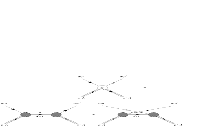
Figure 2: The kinematics for the “particle” propagation

By comparison with eq. (23) one immediately establishes the link

$${G_{\rm p}}(p,p^{\prime};q)={G_{\rm h}}(p,p^{\prime};q^{\prime})~{}.\qquad\qquad q^{\prime}=p+p^{\prime}-q$$ (35)

For sake of simplicity we consider a specific model of a fermionic field interacting with scalar bosonic field $\sigma(y)$, neglecting the self-interactions $\sim\sigma^{3}$ and $\sigma^{4}$. In this simplified scheme (that nevertheless still contains all the difficulties relevant to the fermionic sector) the Hamiltonian of the system reads

$$H=\int d^{3}y\overline{\psi}_{y}\left(-i{\mbox{\boldmath$\gamma$}}{\mbox{\boldmath$\nabla$}}_{y}+m+g\sigma_{y}\right)\psi_{y}+H^{0}_{\sigma}$$ (36)

$H^{0}_{\sigma}$ being the free Hamiltonian of the $\sigma$ meson). Using the equation of motion for the field operator $\psi$

$$\gamma^{0}\left[\psi,H\right]={\mbox{\boldmath$\gamma$}}\left[\psi,\hat{\bf p}\right]+(m+\sigma)\psi$$ (37)

we can derive the evolution equation for $G$, namely

$$\left(i\gamma\cdot\partial_{y}-m\right)G_{pp^{\prime}}(y,y^{\prime})=$$

$$(2\pi)^{3}\delta({\bf p}-{\bf p}^{\prime})\delta^{4}(y-y^{\prime})-i\frac{g}{2\sqrt{p_{0}p_{0}^{\prime}}}<p^{\prime}|{\cal T}\left\{\sigma(y)\psi(y)\overline{\psi}(y^{\prime})\right\}|p>$$

We can first of all prove that, on general grounds, that $G_{pp^{\prime}}(y,y^{\prime})$ can be inverted and consequently a mass operator can be defined by means of a perturbation expansion. The standard proof requires to introduce the generating functional for connected diagrams and then to perform a Légendre transformation on it, and since it can be found in the usual textbooks [13], is not reported here. We only remark that the generalisation of the Green’s function definition used in the present paper will only affect the boundary conditions of the path integral representation of the generating functional, but not the steps needed to define the mass operator.

We rewrite eq. (23) in the form of a Dyson’s-like equation in Fourier transform as

$$\left\{\gamma\cdot(p-q)-m\right\}{G_{\rm h}}(p,p^{\prime};q)=(2\pi)^{3}\delta({\bf p}-{\bf p}^{\prime})$$

$$+\int\frac{d^{3}{p_{1}}}{(2\pi)^{3}}\left[{{\cal M}_{\rm h}}(p,p_{1};q){G_{\rm h}}(p_{1},p^{\prime};q)+{{\cal M}_{\rm p}}(p_{1},p^{\prime};q^{\prime}){G_{\rm p}}(p,p_{1};q^{\prime})\right]~{},$$

the mass operators ${{\cal M}_{\rm h}}$ and ${{\cal M}_{\rm p}}$ being defined according to the “hole” and “particle” channels through

$$\int\frac{d^{3}p_{1}}{(2\pi)^{3}}{{\cal M}_{\rm h}}(p,p_{1};q){G_{\rm h}}(p_{1},p^{\prime};q) =\frac{(2\pi)^{3}}{2\sqrt{p_{0}p_{0}^{\prime}}}<p^{\prime}|\bar{\varphi}\frac{\delta(\hat{\bf p}-{\bf q})}{H-q_{0}-i\alpha}\sigma\varphi|p>$$ (40)

$$\int\frac{d^{3}p_{1}}{(2\pi)^{3}}{{\cal M}_{\rm p}}(p_{1},p^{\prime};q^{\prime}){G_{\rm p}}(p,p_{1};q^{\prime}) =\frac{(2\pi)^{3}}{2\sqrt{p_{0}p_{0}^{\prime}}}<p^{\prime}|\varphi\sigma\frac{\delta(\hat{\bf p}-{\bf q}^{\prime})}{q_{0}-H+i\alpha}\bar{\varphi}|p>$$ (41)

In the above $p$ and $p^{\prime}$, as well as $p_{1}$, are restricted to the mass shell and $\sigma$ is defined as

$$\sigma=\sigma(y)\bigm{|}_{y=0}\quad\Rightarrow\quad\sigma(y)=e^{i\hat{p}y}\sigma e^{-i\hat{p}y}~{}.$$ (42)

Further, the index $h$ in ${{\cal M}_{\rm h}}$ only remind the “hole” kinematics chosen in introducing the Fourier transform. In the configuration space the mass operator is univoquely determined by the Green’s function and embodies both particle and hole propagation.

Concerning the structure of the mass operator, the general theory tells us that it is built by the sum of all 1PI (one-particle-irreducible) diagrams defined in sec. 5 as shown in fig. 3,

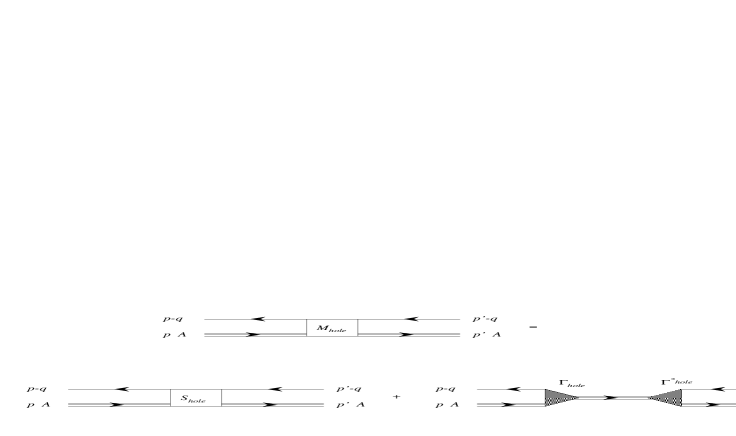
Figure 3: The diagrammatic representation of the Dyson’s mass operator

and must have the analytical structure

$${{\cal M}_{\rm h}}(p,p^{\prime},q)=S_{\rm h}(p,p^{\prime},q)+{\sum\hskip-15.0pt\int}\frac{{\Gamma_{\rm h}}_{n}(p,q){\Gamma_{\rm h}}_{n}^{*}(p^{\prime},q)}{{q_{\rm h}}_{n}({\bf q})-q_{0}-i\alpha}~{}.$$ (43)

Here the first term is a smooth (regular) function of $q_{0}$ while the second term carries poles in $q_{\rm h}$, living of course in the region $q^{2}>M^{2}_{A-1}$. Eq. (3) also shows that a pole of ${{\cal M}_{\rm h}}$ corresponds to a 0 of ${G_{\rm h}}$ and vice versa.

The “particle” mass operator has an analogous expansion but its poles lie in the region $q^{2}>M^{2}_{A+1}$.

The knowledge of the Green’s function (or of the mass operator) gives us access to many observables, like, for instance, the number of baryons

$$\begin{split}A&={\rm Tr}\int\frac{d^{4}q}{(2\pi)^{4}i}\gamma^{0}{G_{\rm h}}(p,p;q)e^{-iq_{0}\alpha}\end{split}$$ (44)

and the ground state energy

$$\begin{split}p_{0}&=\frac{<p|H|p>}{<p|p>}\\ &=-i{\rm Tr}\int\frac{d^{4}q}{(2\pi)^{4}}\Bigl{\{}\left[{\mathbf{\gamma}}\cdot({\bf p}-{\bf q})+m\right]{G_{\rm h}}(p,p;q)\\ &+\int\frac{d^{3}p^{\prime}}{(2\pi)^{3}}{{\cal M}_{\rm h}}(p,p^{\prime};q){G_{\rm h}}(p^{\prime},p;q)\Bigr{\}}+\frac{<p|H_{0}^{\sigma}|p>}{<p|p>}~{}.\end{split}$$ (45)

Now we can introduce the analogous of the “single particle wave functions” in our relativistic approach, generalising what was described by eqs. (7,8). This is done by taking eq. (3) and integrating it over $q_{0}$ in a small circle containing a pole $q_{\lambda 0}$ (within box normalisation if needed) and remembering that the poles of the Green’s function and of the mass operator never coincide. In so doing we immediately find

$$\left\{\gamma(p-q_{\lambda})-m\right\}\varphi_{\lambda}({\bf p},{\bf q}) = \int{d^{3}p^{\prime}\over{2(2\pi)^{3}\sqrt{p_{0}p_{0}^{\prime}}}}{{\cal M}_{\rm h}}(p,p^{\prime};q_{\lambda})\varphi_{\lambda}({\bf p}^{\prime},{\bf q})$$ (46)

$$= \sqrt{M_{\lambda}\over 2p_{0}q_{\lambda 0}}<q_{\lambda}|\sigma\psi|p>~{},$$

$$\left\{\gamma(q_{\nu}-p)-m\right\}\varphi_{\nu}({\bf p},{\bf q}) = \int{d^{3}p^{\prime}\over{2(2\pi)^{3}\sqrt{p_{0}p_{0}^{\prime}}}}{{\cal M}_{\rm p}}(p^{\prime},p;q_{\lambda})\varphi_{\lambda}({\bf p}^{\prime},{\bf q})$$

$$= \sqrt{M_{\nu}\over 2p_{0}q_{\nu 0}}<p|\sigma\psi|q_{\nu}>~{}.$$

The above quantities $\varphi$ are not, of course, wave functions, because they feel the presence in the system of antiparticles as well as of mesons, but can be looked at as eigenfunction of the system. The case of uniformly invariant system (free Fermi gas or maybe quark-gluon plasma) may enable us to make strongly simplifying assumptions. For finite systems we however can still exploit the idea of a mean field calculation.

4 The relativistic shell model

The last equations of the previous section contain the ground idea to build the relativistic analogue of the shell model.

We first consider the “hole” channel and rewrite eq. (46) in the form [14]

$$\left\{\gamma(p-q_{\ell}(q))-m\right\}\varphi_{\ell}(p,q)=\int\frac{d^{3}p^{\prime}}{(2\pi)^{3}}{{\cal M}_{\rm h}}(p,p^{\prime};q)\varphi_{\ell}(p^{\prime},q)$$ (48)

with the subtle difference that now $q_{0}$ is considered a free parameter. If follows that (48) considered at a given $q_{0}$ can be regarded as an eigenvalue equation, the eigenvalue being $q_{\ell 0}(q)$ that is in general different from the $q_{0}$ fixed and contained in ${{\cal M}_{\rm h}}$. Here notations matter: in fact $\varphi_{\ell}$ depends upon the 4-vector $q$, chosen by the exterior. We have left the dependence upon $p$ instead of ${\bf p}$ to remind the reader that $\varphi_{\ell}$ is a 4-spinor depending, furthermore, upon Lorentz-covariant quantities like $q^{2}$ and $p\cdot q$, being understood however that $p_{0}$ is fixed by the mass shell condition.

Having distinguished between $q_{0}$ and the eigenvalue $q_{\ell 0}(q)$, (48) will have a complete orthogonal set of eigenfunction, i.e., the $\varphi_{\ell}$ must obey the properties

$$\int\frac{d^{3}p}{(2\pi)^{3}}\varphi_{\ell^{\prime}}^{*}(p,q)\varphi_{\ell}(p,q) = \delta_{\ell^{\prime}\ell}c_{\ell}(q)$$ (49)

$$\sum_{\ell}\frac{1}{c_{\ell}(q)}\varphi_{\ell}(p,q)\varphi_{\ell}^{*}(p^{\prime},q) = (2\pi)^{3}\delta({\bf p}-{\bf p}^{\prime})\;,$$ (50)

$c_{\ell}(q)$ being a suitable normalisation factor.

Eq. (48) at a fixed and suitably chosen $q_{0}$ looks like a shell model equation having a (non-local) “shell model potential” ${{\cal M}_{\rm h}}$; the functions $\varphi_{\ell}(p,q)$ are not connected with any observable quantities, but they are expected, for a reasonable approximation of ${{\cal M}_{\rm h}}$ and in a convenient range of $q_{0}$ (it means some average of the single particle levels of a shell model well) to approach the “single hole” wave functions $\varphi_{\ell}(p,q)$ previously introduced. This is of course likely below the Fermi level.

For the particle channel we rewrite eq. (3) as

$$\left\{\gamma(Q_{\ell}(q)-p)-m\right\}\chi_{\ell}(p,q)=\int{d^{3}p^{\prime}\over{2(2\pi)^{3}\sqrt{p_{0}p_{0}^{\prime}}}}{{\cal M}_{\rm p}}(p^{\prime},p;q_{\lambda})\chi_{\ell}(p^{\prime},q)~{},$$ (51)

normalisation and completeness relations being fully analogous the “hole wave function” case.

According to the general form (29) we can now introduce the shell-model-like Green’s function as

$$\begin{split}{{\cal G}_{\rm h}^{\rm s.m.}}(p,p^{\prime};q)&=\sum_{\ell}\frac{N_{\ell}}{c_{\ell}(q)}\frac{\varphi_{\ell}(p,q)\overline{\varphi}_{\ell}(p^{\prime},q)}{q_{\ell 0}(q)-q_{0}-i\alpha}\\ &+\sum_{\ell}\frac{(1-N_{\ell})}{d_{\ell}(q^{\prime})}\frac{\chi_{\ell}(p^{\prime},q^{\prime})\bar{\chi}_{\ell}(p,q^{\prime})}{q^{\prime}_{0}-Q_{\ell 0}(q^{\prime})+i\alpha}\Biggm{|}_{q^{\prime}=p+p^{\prime}-q}\end{split}$$ (52)

where $c_{\ell}$ and $d_{\ell}$ are suitable normalisation factors and

$$N_{\ell}=\theta(\ell_{F}-\ell)~{},$$ (53)

with

$$\sum_{\ell}N_{\ell}=A~{}.$$ (54)

Of course the labels $\ell$’s are ordered increasingly with the corresponding energy and $\ell_{F}$ denotes the highest occupied level (Fermi level).

The equation the function ${{\cal G}_{\rm h}^{\rm s.m.}}(p,p^{\prime};q)$ fulfils is similar to (3), provided the $\delta$ function in the r.h.s. is replaced by

$$\sum_{\ell}\gamma_{0}\left\{\frac{N_{\ell}}{c_{\ell}(q)}\varphi_{\ell}(p,q)\overline{\varphi}_{\ell}(p^{\prime},q)+\frac{1-N_{\ell}}{d_{\ell}(q^{\prime})}\chi_{\ell}(p^{\prime},q^{\prime})\bar{\chi}_{\ell}(p,q^{\prime})\right\}~{}.$$

The above is of course expected to approximate a $\delta$ as far as the “shell model” approximation holds valid.

In the above formalism clearly the poles of ${\cal G}_{\rm hole}$ must also be poles of ${{\cal G}_{\rm h}^{\rm s.m.}}$ (the converse is not true in general because some poles of ${G_{\rm h}}$ are killed by the projection operator $1-N_{\ell}$).

We assume that the equations

$$q_{\ell 0}(q_{\lambda_{\ell}}) = q_{\lambda_{\ell}0}({\bf q})$$ (55)

$$Q_{\ell 0}(q_{\nu_{\ell}}) = q_{\nu_{\ell}0}({\bf q})$$ (56)

have one or more (maybe infinite) roots for a given “single particle” quantum number $\ell$. The $q_{\lambda_{\ell}0}({\bf q})$ are the eigenvalues of the equation for the $A-1$ particle state

$$H|q_{\lambda_{\ell},\nu_{\ell}}>=q_{\lambda_{\ell}\nu_{\ell}0}|q_{\lambda_{\ell},\nu_{\ell}}>\;.$$ (57)

The residua of ${G_{\rm h}}$ and of ${{\cal G}_{\rm h}^{\rm s.m.}}$ below the Fermi level coincide and from eq. (24) and (52) we obtain

$$\varphi_{\lambda_{\ell}}({\bf p},{\bf q})\overline{\varphi}_{\lambda_{\ell}}({\bf p}^{\prime},{\bf q})=\frac{N_{\ell}}{c_{\ell}(q)}\left\{1-\frac{\partial q_{\ell 0}(q)}{\partial q_{0}}\right\}^{-1}\varphi_{\ell}(p,q)\overline{\varphi}_{\ell}(p^{\prime},q)\Biggm{|}_{q_{0}=q_{\lambda 0}({\mathbf{q}})}$$ (58)

Thus the above suggests to attribute to the $\varphi_{\lambda_{\ell}}$ the meaning of a generalisation at the relativist level of a single particle wave function in a shell model, fully maintaining, nevertheless, Lorentz and Poincaré invariance. We repeat once more that this occurs because we are considering a “non-diagonal” single-particle Green’s function where the recoil of the daughter nucleus is accounted for.

Now we make a physical assumption that further narrows us to the shell model: we assume that a one particle level $\ell$ is composed by the same sub-levels $\lambda_{\ell}$ of the exact many-body problem in such a way that

$$\sum_{\lambda_{\ell}}\int\frac{d^{3}q}{(2\pi)^{3}}\left|\varphi_{\lambda_{\ell}}({\bf p},{\bf q})\right|^{2}$$

$$=\sum_{\lambda_{\ell}}\int\frac{d^{3}q}{(2\pi)^{3}}\frac{N_{\ell}}{c_{\ell}(q)}\left\{1-\frac{\partial q_{\ell 0}(q)}{\partial q_{0}}\right\}^{-1}\left|\varphi_{\ell}(p,q)\right|^{2}\Biggm{|}_{q_{0}=q_{\lambda_{\ell}0}({\mathbf{q}})}=N_{\ell}~{}^{\prime}$$

This property is not peculiar of a relativistic system, since the same will happen in the non-relativistic case.

Now we are ready to make the last step and introduce a phenomenological “shell model” potential $V(p,p^{\prime};\tilde{q})$, with $p$ and $p^{\prime}$ restricted to the nucleus mass shell and the 4-vector $\tilde{q}$ chosen as

$$\tilde{q}=(\tilde{q}_{0},{\bf q})~{},~{}~{}~{}~{}~{}~{}~{}~{}~{}~{}~{}\tilde{q}_{0}=\sqrt{{\bf q}^{2}+M^{2}_{A-1}}~{},$$ (60)

where $M_{A-1}$ is the mass of the daughter nucleus in its ground state (this choice maintains the analogy with the non-relativistic case: see, e.g., [14])

Thus the potential $V$ is independent from $q_{0}$ and we assume it to be symmetric, i.e., $V(p,p^{\prime};{\bf q})=V(p^{\prime},p;{\bf q})$. From now on we must guess $V(p,p^{\prime};{\bf q})$ on phenomenological grounds in such a way that

$$\begin{split}\left\{\gamma(p-q_{\ell}(q))-m\right\}\varphi_{\ell}(p,{\bf q})&-\int\frac{d^{3}p^{\prime}}{(2\pi)^{3}}V(p,p^{\prime};{\bf q})\varphi_{\ell}(p^{\prime},{\bf q})\\ &=\int\frac{d^{3}p^{\prime}}{(2\pi)^{3}}\left[{{\cal M}_{\rm h}}(p,p^{\prime};q)-V(p,p^{\prime};{\bf q})\right]\varphi_{\ell}(p^{\prime},q)\end{split}$$ (61)

will be reasonably small.

Once a parameterisation for $V$ has been given we can write down the eigenvalue equation for the“hole wave functions”

$$\left\{\gamma\cdot(p-q_{\ell}({\bf q}))-m\right\}\varphi_{\ell}(p,{\bf q})=\int\frac{d^{3}p^{\prime}}{(2\pi)^{3}}V(p,p^{\prime};{\bf q})\varphi_{\ell}(p^{\prime},{\bf q})$$ (62)

being

$$q_{\ell}=(q_{\ell 0}({\bf q}),{\bf q})~{},\qquad p=(p_{0}({\bf p}),{\bf p})~{},\qquad p^{\prime}=(p_{0}^{\prime}({\bf p^{\prime}}),{\bf p^{\prime}})~{}.$$ (63)

The index $\ell$ (of course discrete) summarises now all the quantum numbers pertaining to a given “one-hole” state in the “shell model potential” $V$.

As an aside, in analogy with the “hole” channel, we can introduce an equation for the “particle” channel as

$$\left\{\gamma\cdot(Q_{\ell}({\bf q})-p)-m\right\}\chi_{\ell}(p,{\bf q})=\int\frac{d^{3}p^{\prime}}{(2\pi)^{3}}V(p,p^{\prime};{\bf q})\chi_{\ell}(p^{\prime},{\bf q})~{}.$$ (64)

Up to now covariance has been preserved. The next step is to find a practical way to solve the “shell model equation” (62). Since it is not so easy to give an explicit solution of it in a covariant form, we are forced, in the following, to choose a suitable reference frame where the equation is particularly simple. Once the solution has been found, however, we need a procedure to boost it to any reference frame. This will be our next task.

Thus, coming to the “hole” channel, there are two natural choice for the reference frame. One is to assume it as the rest frame for the $A-1$ system, i.e., ${\bf q}=0$: the eigenvalue equation there becomes

$$\left\{\gamma\cdot k_{\ell}-m\right\}\varphi(k,0)=\int\frac{d^{3}k^{\prime}}{(2\pi)^{3}}V(k,k^{\prime})\varphi(k^{\prime},0)$$ (65)

where

$$k_{\ell}=(p_{0}({\bf k})-q_{\ell 0},{\bf k})~{},\qquad k=(p_{0}({\bf k}),{\bf k})~{},\qquad k^{\prime}=(p_{0}({\bf k}^{\prime}),{\bf k}^{\prime})~{}.$$ (66)

Another customary choice is to assume ${\bf p}=0$ (rest frame for the $A$-nucleons system). Of course any reference frame can be reached by means of a boost. Thus let $|0>$ be the ${\bf p}=0$ frame and let $\Lambda$ be the boost from $|0>$ to the state $|k>$ corresponding to ${\bf q}=0$:

$$|k>=\Lambda|0>~{}.$$

Let us specify in more details the state of the daughter nucleus: we expand the previous index $\ell$ as

$$\ell\equiv(\lambda,J,M,\pi)$$

where $J$ is the total angular momentum, $M$ its third component and $\pi$ the parity. $\lambda$ will then resume all the other intrinsic (not frame-dependent) quantum numbers. We can now write

$$\begin{split}\varphi_{\lambda,J,M,\pi}({\bf k},0)&=\frac{1}{\sqrt{2p_{0}({\bf k})}}<0;\lambda,J,M,\pi|\psi(0)\Lambda|0>\\ &=\frac{1}{\sqrt{2p_{0}({\bf k})}}<0;\lambda,J,M,\pi|\Lambda\Lambda^{-1}\psi(0)\Lambda|0>\\ &=\frac{1}{\sqrt{2p_{0}({\bf k})}}S(-{\bf v})<-\eta_{\lambda}{\bf k};\lambda,J,M,\pi|\psi(0)|0>\end{split}$$ (67)

where as usual $S$ is defined through the relation

$$S(-{\bf v})\psi(0)=\Lambda^{-1}\psi(0))\Lambda$$ (68)

and reads

$$S(-{\bf v})=\sqrt{\frac{p_{0}({\bf k})+M}{2M}}\left(1-\frac{\gamma^{0}{\boldsymbol{\gamma}}\cdot{\bf k}}{p_{0}({\bf k})+M}\right)~{}.$$ (69)

Of course

$${\bf v}=\frac{\bf k}{p_{0}({\bf k})}$$ (70)

denotes the velocity of the boost from the rest frame of the daughter nucleus and an extra factor accounting for the mass difference between the $A$ and $A-1$ systems is required, namely

$$\eta_{\lambda}=\frac{M^{A-1}_{\lambda,J,\pi}}{M}~{}.$$ (71)

The above entails

$$\Lambda^{-1}|0;\lambda,J,M,\pi>=|-\eta_{\lambda}{\bf k};\lambda,J,M,\pi>~{}.$$ (72)

In the ${\bf p}=0$ frame the 4-vector $q$ transforms into

$$q^{\prime}_{0}\frac{M^{A-1}_{\lambda,J,\pi}}{\sqrt{1-v^{2}}} = \frac{M^{A-1}_{\lambda,J,\pi}}{M}p_{0}({\bf k})=\sqrt{(M^{A-1}_{\lambda,J,\pi})^{2}+\eta_{\lambda}^{2}{\bf k}^{2}}$$ (73)

$${\bf q}^{\prime} = -\frac{{\bf v}M^{A-1}_{\lambda,J,\pi}}{\sqrt{1-v^{2}}}=-\eta_{\lambda}{\bf k}$$ (74)

and the “eigenfunction” $\varphi$ reads

$$\begin{split}\varphi_{\lambda,J,M,\pi}(0,{\bf k})&=\sqrt{\frac{M^{A-1}_{\lambda,J,\pi}}{2Mq_{\lambda JM\pi;0}({\bf k})}}<{\bf k};\lambda,J,M,\pi|\psi(0)|0>\\ &=S(-{\bf v}_{\lambda})\varphi_{\lambda,J,M,\pi}(-{\bf k}/\eta_{\lambda},0)\end{split}$$ (75)

with

$${\bf v}_{\lambda}=\frac{{\bf k}}{q_{\lambda JM\pi;0}({\bf k})}~{}.$$ (76)

This definitions implies

$$\int\frac{d^{3}k}{(2\pi)^{3}}\overline{\varphi}_{\lambda,J,M,\pi}(0,{-\bf k})\varphi_{\lambda,J,M,\pi}(0,{\bf k})\\ =\eta_{\lambda}^{2}\int\frac{d^{3}k}{(2\pi)^{3}}\overline{\varphi}_{\lambda,J,M,\pi}({\bf k},0)\varphi_{\lambda,J,M,\pi}({\bf k},0)~{}.$$ (77)

The formalism above has shown that we can solve the “shell model” equation (62) in the rest frame for the $A-1$ daughter nucleus and then, using the above kinematics, transfer the solutions to the usual rest frame of the $A$ nucleus, namely ${\bf p}=0$. Having established good transformation properties of the solutions, we now need to find them in the preferred reference system. Before doing explicit (model) calculations let us investigate a little what lies beyond the shell model.

5 The perturbative expansion

The shell model in nuclear physics is usually thought as the 0^th order (mean field) of a perturbation expansion. Using the eigenfunctions derived from eqs. (62) and (64) we can represent the “unperturbed” Green’s function in the “hole” kinematic, in analogy with (52), as

$$\begin{split}G_{\rm h}^{0}(p,p^{\prime};q)&=\sum_{\ell}\frac{N_{\ell}}{c_{\ell}(q)}\frac{\varphi_{\ell}(p,{\bf q})\overline{\varphi}_{\ell}(p^{\prime},{\bf q})}{q_{\ell 0}({\bf q})-q_{0}-i\alpha}\\ &+\sum_{\ell}\frac{1-N_{\ell}}{d_{\ell}(q^{\prime})}\frac{\chi_{\ell}(p^{\prime},{\bf q}^{\prime})\bar{\chi}_{\ell}(p,{\bf q}^{\prime})}{q^{\prime}_{0}-Q_{\ell 0}({\bf q}^{\prime})+i\alpha}\Biggm{|}_{q^{\prime}=p+p^{\prime}-q}\end{split}$$ (78)

Also, we can introduce a “shell-model particle Green’s function” by applying the relation (3) to eq. (78), namely

$$G^{0}_{\rm p}(p,p^{\prime};q)=G^{0}_{\rm h}(p,p^{\prime};p+p^{\prime}-q)~{}.$$ (79)

The first order in the expansion of the mass operator ${\cal M}$ in terms of the meson interaction coincides the Hartree-Fock approximation: the first contribution reads

$$\begin{split}({{\cal M}_{\rm h}})_{\rm Hartree}&=-i{\rm Tr}g^{2}\int\frac{d^{4}k}{(2\pi)^{4}}{G_{\rm h}}^{0}(p,p^{\prime},k){\cal D}_{0}(p-p^{\prime})\\ &={\rm Tr}\sum_{l}g^{2}\int\frac{d^{3}k}{(2\pi)^{3}}\overline{\varphi}_{\ell}(p^{\prime},{\bf q})\varphi_{\ell}(p,{\bf q})D_{0}(p-p^{\prime})\end{split}$$ (80)

where of course

$${\cal D}_{0}(k)=\frac{1}{k^{2}-m^{2}_{\sigma}+i\alpha}$$ (81)

is the free $\sigma$ propagator, and is displayed in fig. 4,

Figure 4: Diagrammatic description of the Hartree contribution to the mass operator

while the second term represents, as one can easily convince himself, the Fock contribution, namely

$$({{\cal M}_{\rm h}})_{\rm Fock}=i{\rm Tr}g^{2}\int\frac{d^{4}k}{(2\pi)^{4}}{G_{\rm h}}^{0}(p,p^{\prime},k){\cal D}_{0}(k-q)~{}.$$ (82)

and is represented in fig. 5,

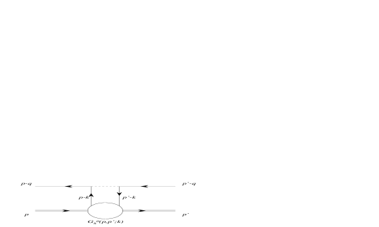
Figure 5: Diagrammatic description of the Fock contribution to the mass operator

The other terms have complicated and in practice non manageable expressions that involve the detailed structure (i.e., the excited states) of the target nucleus. We only show diagrammatically a second order contribution in fig. 6.

6 A simple model

The above theory looks rather formal. Thus let us show how it can be implemented in a practical case. In order to have manageable formulas we consider a “shell model potential” of the separable form

$$V({\bf k},{\bf k}^{\prime})=-(2\pi)^{3}\sum_{Jlj}Y_{Jlj}({\bf k})Y_{Jlj}^{\dagger}({\bf k}^{\prime})v_{J}(|{\bf k}|)v_{J}(|{\bf k}^{\prime}|)$$ (83)

where as usual

$$Y_{Jlj}({\bf k})=\sum_{s}<l,j-s;\frac{1}{2},s|l,\frac{1}{2};J,j>Y_{lj-s}({\bf k})\chi_{s}$$

are the generalised spherical harmonics and $v_{J}$ is some function to be chosen in such a way to reproduce the nuclear phenomenology. Actually we put

$$v_{J}(|{\bf k}|)=\left(\frac{c}{m^{2}+{\bf k}^{2}}\frac{1}{b+e^{ka(A,J)}}\right)^{\frac{1}{2}}$$ (84)

where $b$ an $c$ are constant and $a(A,J)$ will depend upon the atomic number $A$ and, a priori, upon the total angular momentum $J$.

Now we can solve eq. (65) (we assume that, as established in sec. 4, once the eigenfunctions $\varphi_{n}$ have been found in the frame of reference ${\bf q}=0$ then the above described transformations can provide their expression in any other frame).

The spinor (not strictly speaking a wave function) solution of (65) will be labelled by $J$ and $\omega$ and has the form

$$\varphi_{J,\omega}=\begin{pmatrix}Y_{Jlj}(\hat{\bf k})F_{J,\omega}(k)\\ Y_{Jl^{\prime}j}(\hat{\bf k})G_{J,\omega}(k)\end{pmatrix}$$ (85)

where

$$l=J+\frac{\omega}{2}~{},\qquad\qquad\qquad l^{\prime}=J-\frac{\omega}{2}$$

and

$$\omega=\begin{cases}+1&\text{for~{}states~{}with~{}parity~{}}(-1)^{J+\frac{1}{2}}\\ -1&\text{for~{}states~{}with~{}parity~{}}(-1)^{J-\frac{1}{2}}\end{cases}~{}.$$ (86)

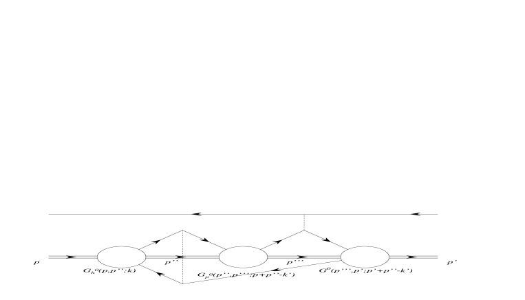
Figure 6: A typical example of higher order diagram in a perturbative calculation

Using the well known relation (independent of the parity)

$${\boldsymbol{\sigma}}\cdot{\bf k}Y_{Jlj}(\hat{\bf k})=-kY_{Jl^{\prime}j}(\hat{\bf k})$$ (87)

we find

$$(k\cdot\gamma-m)\varphi_{J,\omega}=\begin{pmatrix}\left[(k_{0}-m)F_{J,\omega}(k)+kG_{J,\omega}(k)\right]Y_{Jlj}(\hat{\bf k})\\ -\left[kF_{J,\omega}(k)+(k_{0}+m)G_{J,\omega}(k)\right]Y_{Jl^{\prime}j}(\hat{\bf k})\end{pmatrix}$$ (88)

and now not only eq. (65) is separable thanks to the choice of the potential but the large and small components of the spinors are decoupled and one gets

$$(k_{0}-m)F_{J,\omega}(k)+kG_{J,\omega}(k)&=-v_{J}(k)X_{J}[F_{J,\omega}]\\ -kF_{J,\omega}(k)-(k_{0}+m)G_{J,\omega}(k)=-v_{J}(k)X_{J}[G_{J,\omega}]$$ (89)

where the functional $X_{J}$ is defined as

$$X_{J}[f]=\int\limits_{0}^{\infty}p^{2}dp\,v_{J}(p)f(p)~{}.$$ (90)

Then inverting the above and recalling (66), i.e., expliciting the expression of the eigenvalue $k_{0}=p_{0}({\bf k})-q_{\ell 0}$, we get the system

$$F_{J,\omega}(k)&=-\frac{(p_{0}({\bf k})-q_{\ell 0}+m)X_{J}[F_{J,\omega}]+kX_{J}[G_{J,\omega}]}{(p_{0}({\bf k})-q_{\ell 0})^{2}-k^{2}-m^{2}}v_{J}(k)~{},\\ G_{J,\omega}(k)=\frac{kX_{J}[F_{J,\omega}]+(p_{0}({\bf k})-q_{\ell 0}-m)X_{J}[G_{J,\omega}]}{(p_{0}({\bf k})-q_{\ell 0})^{2}-k^{2}-m^{2}}v_{J}(k)~{}.$$ (91)

Inserting then these expressions into the definition of the functionals $X_{J}[F_{J,\omega}]$ and $X_{J}[G_{J,\omega}]$ we get for them a homogeneous system, namely

$$X_{J}[F_{J,\omega}]&=B^{-}_{J}(q_{\ell 0})X_{J}[F_{J,\omega}]-C_{J}(q_{\ell 0})X_{J}[G_{J,\omega}]~{},\\ X_{J}[G_{J,\omega}]=C_{J}(q_{\ell 0})X_{J}[F_{J,\omega}]-B^{+}_{J}(q_{\ell 0})X_{J}[G_{J,\omega}]$$ (92)

where we have defined

$$B^{\pm}_{J}(q_{\ell 0}) = \int\limits_{0}^{\infty}k^{2}dk\frac{\left[q_{\ell 0}-p_{0}({\bf k})\pm m\right]v^{2}_{J}(k)}{(p_{0}({\bf k})-q_{\ell 0})^{2}-k^{2}-m^{2}}~{},$$ (93)

$$C_{J}(q_{\ell 0}) = \int\limits_{0}^{\infty}k^{3}dk\frac{v^{2}_{J}(k)}{(p_{0}({\bf k})-q_{\ell 0})^{2}-k^{2}-m^{2}}~{}.$$ (94)

The eigenvalue equation generated from the system (92) is then

$$R_{J}(q_{\ell 0})=[C_{J}(q_{\ell 0})]^{2}-(B^{-}_{J}(q_{\ell 0})-1)(B^{+}_{J}(q_{\ell 0})+1)=0~{}.$$ (95)

Note that the functions $B^{\pm}_{J}$ and $C_{J}$ are real only in the range $q_{\ell 0}>M_{A}+m$ or $q_{\ell 0}<M_{A}-m$, (the former case referring to a $A$-nucleus system plus an antinucleon and the latter to a $A$-nucleus plus a hole). Here of course $M_{A}=p_{0}(0)$ denotes the rest mass of the $A$-nucleus.

Once the equation is solved in $q_{\ell 0}$ we also get, up to a normalisation constant, the explicit expressions for the “wave functions”

$$F_{J,\omega}(k)&=-\frac{p_{0}({\bf k})-(q_{\ell 0}+m)C_{J}(q_{\ell 0})-k(1-B^{-}_{J}(q_{\ell 0}))}{(p_{0}({\bf k})-q_{\ell 0})^{2}-k^{2}-m^{2}}v^{2}_{J}(k)~{},\\ G_{J,\omega}(k)=\frac{-(p_{0}({\bf k})-q_{\ell 0}-m)(1-B^{-}_{J}(q_{\ell 0}))+kC_{J}(q_{\ell 0})}{(p_{0}({\bf k})-q_{\ell 0})^{2}-k^{2}-m^{2}}v^{2}_{J}(k)~{}.$$ (96)

Note that, from (95), the energy levels are degenerate with respect to $j$ and to the parity and in the notations we can rewrite $q_{\ell 0}$ as $q_{J0}$.

If we further introduce the notation

$$\varepsilon=M_{A}-q_{J0}-m$$ (97)

then the functions $B^{\pm}$ and $C$ become

$$B^{+}(\varepsilon)= -\int\limits_{0}^{\infty}k^{2}dk\frac{\Delta p+\varepsilon}{(\Delta p+\varepsilon)(\Delta p+\varepsilon+2m)-k^{2}}v^{2}_{J}(k)$$ (98)

$$B^{-}(\varepsilon)= -\int\limits_{0}^{\infty}k^{2}dk\frac{\Delta p+\varepsilon+2m}{(\Delta p+\varepsilon)(\Delta p+\varepsilon+2m)-k^{2}}v^{2}_{J}(k)$$ (99)

and

$$C(\varepsilon))= \int\limits_{0}^{\infty}k^{2}dk\frac{1}{(\Delta p+\varepsilon)(\Delta p+\varepsilon+2m)-k^{2}}v^{2}_{J}(k)$$ (100)

where we put

$$\Delta p=p_{0}({\bf k})-M_{A}$$ (102)

to better control the orders-of-magnitude: this last quantity is in fact expected to be small (say, of the order of $k^{2}/2M_{A}$) unless we look to extreme situations, and for bound states $\varepsilon$ is of the order of few $MeV$.

To exemplify how the above works, we have chosen the parameters in (84) as

$$a(A,J)&=\frac{1}{m}\left[0.7314+0.3274A^{\frac{1}{3}}-0.0884^{\frac{2}{3}}+0.0089A-0.005(2J-1)\right]\\ ~{}\\ b=0.09\\ c=0.1$$ (103)

and we have evaluated the hole energy for different values of $A$ and $J$. The results (in MeV) are reported in table 1.For sake of simplicity we have assumed

$$M_{A}=A(m+\mu)$$ (104)

and the chemical potential $\mu$ is chosen as usual as $\mu=-8$ MeV.

A	$J=1/2$	$J=3/2$	$J=5/2$	$J=7/2$	$J=9/2$
12	-9.5	-8
24	-10.5	-9	-8
40	-12.5	-10.5	-9	-8
60	-15	-13	-11.5	-10	-8

Table 1: Energy levels of the relativistic “shell model” for different $A$ and $J$

The above example shows how our formalism works. To our knowledge the approach presented in this paper is beyond the usual relativistic shell calculations, since the usual ways to afford relativity (see our ref. [3] and the many references quoted therein) mainly concern QHD (Quantum-Hadro-Dynamics) inspired models with a space-dependent mass term that explicitly breaks Poincaré invariance. This flaw is obviously not obnoxious when heavy nuclei are concerned, it has no future however when handling a nucleon as a 3-quark system.

7 Conclusion and outlook

In the present paper we have shown how a relativistic theory of the nucleus can be constructed still preserving the main features of the shell model. In our approach in fact a shell model like equation has been constructed, admittedly in a well defined reference frame, but we have also built up all the formalism needed to boost the results to any other frame of reference, thus reconstructing Lorentz and Poincaré invariance: this is a by far non-trivial achievement, since in the traditional nuclear physics translational invariance is broken from the very beginning by the shell model even in a non-relativistic scheme. Of course the above is particularly suitable for small systems, since recoil and center-of-mass motion is fully accounted for. This goes clearly beyond the approaches based on translationally invariant systems[2, 5].

Of course some approximations can be needed in practical calculations, and mainly we introduce a “shell-model potential” which is thought to approximate the mass operator. Again, exactly as described in sec. 2 we can use the same potential to describe particle and hole dynamics, but still the same disease survives, since in principle the mass operator in the “hole” and “particle” kinematics are intrinsically different. Thus we can use the same potential as a starting point, but then different perturbative expansions are required, as shown in sec. 5.

The key issue of the paper is the definition of the “shell model wave function”: we systematically use quotation marks in referring this quantity because it is not at all a wave function, but is defined, instead, as the expectation value between physical states (containing any kind of particles, namely nucleons, mesons and antinucleons) of some field operators. Thus these quantities, referred to in the above as $\varphi$ and $\chi$, maintain the formal analogy with the the true nuclear wave functions of the non-relativistic shell model, but contain a much more involved dynamics, since as many mesons and antinucleons as possible are allowed to appear, and hence accounted for, inside $\varphi$ and $\chi$, the only constraint being a variation of the baryonic number of $\mp 1$.

Thus we can apply the formalism developed so far to any relativistic system, not necessarily to nuclei, but also (as obvious) to nucleons, where the “shell model wave function” (still with quotation marks!) can be regarded as the analogous of the quark wave functions in the constituent quark model, not disregarding, however, the parton content of the constituent quark, which is a composite object built up on current quarks,antiquaks and gluons.

Our formalism can also be regarded as a theoretical ground for the constituent quark model and at the same time shows its limitations: in fact, as shown above, we can derive from the $\varphi$ and $\chi$ the static properties of the nucleus or of the nucleon, but the response functions (in the nuclear case) or the $\gamma$ or lepton interaction with a nucleon require a more detailed study, since the degrees of freedom embodied in the “shell model wave function” require to be explicitly dealt with. We plan in a successive work to explore the dynamical properties of a relativistic complex but finite system.

References

[1]
B. D. Serot and J. D. Walecka.
.
Adv. in Nucl. Phys, 16:1, 1986.
[2]
L. S. Celenza and C. M. Shakin.
Relativistic Nuclear Physics.
World Scientific, Singapore, 1986.
[3]
M. Rashdan.
.
Phys. Rev., C63:044303, 2001.
[4]
W. M. Alberico et al.
.
Phys. Rev., C38:1801, 1988.
[5]
R. Cenni, T. W. Donnelly and A. Molinari.
.
Phys. Rev., C56:276, 1997.
[6]
R. Cenni and G. Vagradov.
.
Nucl. Phys., A587:675, 1995.
[7]
H. Feshbach.
.
Ann. Phys., 5:357, 1958.
[8]
H. Feshbach.
.
Ann. Phys., 19:287, 1962.
[9]
J. S. Bell and E. J. Squires.
.
Phys. Rev. Lett., 3:96, 1959.
[10]
R. Cenni, C. Ciofi degli Atti and G. Salmè.
.
Phys. Rev., C39:1425, 1989.
[11]
A. Molinari and G. Vagradov.
.
Zeitschrift für Physik, A332:119, 1989.
[12]
R. Cenni, A. Molinari and G. Vagradov.
.
Nuovo Cimento, 107A:407, 1994.
[13]
D. J. Amit.
Field Theory, the Renormalization Group, and Critical
Phenomena.McGraw Hill, New York, 1978.
[14]
A. B. Migdal.
theory of Finite Fermi System.
J. Wiley & Sons, New York, London, Sydney, 1967.