Microscopic analysis of $K^{+}$-nucleus elastic scattering based on $K^{+}$-nucleon phase shifts

Abstract

We investigate $K^{+}$-nucleus elastic scattering at intermediate energies within a microscopic optical model approach. To this effect we use the current $K^{+}$-nucleon (KN) phase shifts from the Center for Nuclear Studies of the George Washington University as primary input. First, the KN phase shifts are used to generate Gel’fand-Levitan-Marchenko real and local inversion potentials. Secondly, these potentials are supplemented with a short range complex separable term in such a way that the corresponding unitary and non-unitary KN $S$ matrices are exactly reproduced. These KN potentials allow to calculate all needed on- and off-shell contributions of the $t$ matrix, the driving effective interaction in the full-folding $K^{+}$-nucleus optical model potentials reported here. Elastic scattering of positive kaons from ⁶Li, ¹²C, ²⁸Si and ⁴⁰Ca are studied at beam momenta in the range 400-1000 MeV/$c$, leading to a fair description of most differential and total cross section data. To complete the analysis the full-folding model, three kinds of simpler $t\rho$ calculations are considered and results discussed. We conclude that conventional medium effects, in conjunction with a proper representation of the basic KN interaction are essential for the description of $K^{+}$-nucleus phenomena.

I Introduction

Over the past two decades the study of $K^{+}$-nucleus (KA) collisions with light targets received considerable attention both experimentally and theoretically Fri97 ; Fri97b ; Ker00 . This has been so mainly in virtue of the smooth energy dependence, the relative weak strength of the $K^{+}$-nucleon (KN) interaction and the strangeness of projectile. Herewith, it was expected and largely confirmed that intermediate energy $t\rho$ optical potentials would suffice to describe the scattering data. However, some unexpected and persistent shortcomings were observed in the description of total cross section data, taken in transmission experiments at beam momenta in the range 500-1000 MeV/$c$ Kra92 ; Fri97 ; Fri97b . This situation has triggered outlook for new physics with models including unconventional as well as higher order effects Mard90 ; Che99 . As an important and unsatisfactory element, in all these discussions and up to now, remains the absolute normalization error of the measured cross sections, being $\pm 17$% Ker00 . To mention a few of these efforts, viz covariant formulation Ker00 ; Che99 , consideration of medium modifications of the KN interaction within the target nucleus environment Cai95 ; Cai96 , the use of on- and off-shell $t$-matrix contributions with the construction of separable scattering amplitudes Jia95 , and the possible manifestation of $\Theta^{+}$ pentaquark in KA collissions Gal05 .

The microscopic optical model potential (OMP) approach we present here embodies most of the above elements but puts emphasis on the best possible direct use of KN phase shift data to the generate on- and off-shell KN $t$-matrix elements. This is achieved with the construction of a KN potential, in true sense a KN optical model potential when the respective $S$ matrix is non unitary, which reproduces in absolute terms the phase shift data. This approach distinguishes several steps. First, for each partial wave and set of KN data, an optimal Gel’fand-Levitan-Marchenko inversion potential $V_{\alpha}(r)$ is calculated San97 ; Fun01 . Second, a short range rank-one separable potential, with energy dependent and possibly complex strengths, is added to $V_{\alpha}(r)$ and matched to the data Fun01 . These potentials are used in Lippmann-Schwinger equations for the KN $t$ matrix, the defined effective interaction in the full-folding optical model approach discussed here. These folding calculations are carried out in momentum space with the use of nonlocal single particle target densities. Herein, the full-folding calculations use only the KN $t$ matrix and thus neglect the Pauli blocking in the propagation of nucleons in the nucleus Are02 .

This article is organized as follows. In Section II we summarize the main relativistic considerations in the definition of the bare KN potential. We also outline some aspects of quantum inverse scattering relevant to our applications, specify the KN data and discuss the implied features in the KN interaction. In Section III we present the salient features of the full-folding KA optical potential and discuss three alternative $t\rho$ approximations. In Section IV we show and discuss KA elastic scattering applications for selected nuclei. In section V we present a summary and conclusions of this analysis.

II The KN effective interaction

We base our study on the current KN partial wave phase shift solutions, single and continuous energy solutions for $0<T_{\textrm{Lab}}<1$GeV, of Richard Arndt et al. and retrieved data from Center for Nuclear Studies (CNS) of the George Washington University (GWU) SAID ; Hyl92 . These data are sufficient to specify the partial wave $S$ matrix or $t$ matrix on shell. However, these quantities alone are insufficient in the context of the many-body approach since the KA optical model requires the $t$ matrix off shell. Thus, the problem is ill posed and requires a theoretical extension of the on-shell $t$-matrix into the off-shell domain. The solution to this problem is not unique. However, since our analysis hinges upon a potential theory we chose a KN potential concept also for this purpose. The off-shell extension of the $t$-matrix interaction takes into account free particle propagation, counted to all orders in the ladder approximation, but without KA medium effects. We calculate the $t$ matrices with a Lippmann-Schwinger equation in momentum space.

A well established and often applied link between phase shifts and potential is the inverse scattering formalism of Gel’fand-Levitan and Marchenko. The present application points towards use of the fixed angular momentum or partial wave Schrödinger-type equation version, mathematically speaking Sturm-Liouville equation, yielding energy independent and local potentials San97 . Before we enter into the more technical aspects of inversion it appears useful to recall the relativistic aspects which we associate with the relative motion Schrödinger-type equation being used for the KN pair in the C.M. system.

To formulate the relativistic Hamiltonian description of quantum mechanical particle sytems, the standard rules for constructing the momenta from the Lagrangian cannot be applied when the Lagrangian is singular and the set $(q,\dot{q})$ and $(q,p)$ are not uniquely related. A Lagrangian is singular when the Hessian vanishes,

$$det\left(\frac{\partial^{2}L}{\partial\dot{q}_{i}\partial\dot{p}_{j}}\right)=0.$$ (1)

In such a case it is not possible to simply eliminate the velocity dependences by coordinates and momenta. In order to obtain a Hamiltonian, which depends on coordinates and momenta only, it requires additional independent constraining relations $\phi(q,p)_{j}\approx 0$ to achive uniqueness. Dirac gave very general rules to construct the Hamiltonian and calculated sensible brackets that can be used to describe classical and quantum mechanical dynamics dir64 . These rules are generally known as Dirac’s constraint dynamics. Out of several, an instant form dynamics, developed and used by Crater and Van Alstine cra90 ; liu03 , is used herein to foster the relativistic nature of the partial wave equation which we use in phase shift inversion.

The Hamiltonian is obtained by a Legendre transformation of the Lagrangian, where all primary constraints are multiplied by arbitrary functions of time $\lambda_{j}$ and added to $H$. This yields the total Hamiltonian ${\mathcal{H}}$,

$${\mathcal{H}}=H+\sum_{j=1}^{M}\lambda_{j}\phi_{j}(q,p).$$ (2)

For consistency, the constraints must not change under a time evolution

$$\dot{\phi}_{j}=[\phi_{j},{\mathcal{H}}]\approx 0.$$ (3)

Therefrom three cases are distinguised: an equation can give an identity, it can give a linear equation for the $\lambda_{j}$ or it gives an equation containing selectively $p$ and $q$, in which case it must be considered as another constraint. The constraints that arise from this procedure are called secondary. Also, any linear combination of constraints is again a constraint.

Crater et al. cra90 ; liu03 studied the relativistic 2-particle dynamics as a problem with constraints of the kind

$$\phi_{i}(q,p):=m_{i}^{2}+p^{2}_{i}+\Phi_{i}(q,p,s),\quad i=1,2,$$ (4)

where, in view of the final result, we adopted their metric i.e. using the other sign in the four product, $g_{\mu\mu}=(-1,1,1,1)$. The two constraints are limited to yield $\phi_{i}(q,p)\approx 0$, being generalized mass shell constraints for the two particles.

$$\mathcal{H}_{i}=p_{i}^{2}+m_{i}^{2}+\Phi_{i}(x,p_{1},p_{2})\approx 0,\quad i=1,2,$$ (5)

where $(\mathcal{H}_{1},\mathcal{H}_{2})$ are covariant constraints on the four momenta $(p_{1},p_{2})$. The interaction functions $(\Phi_{1},\Phi_{2})$ being equal, $\Phi_{1}=\Phi_{2}$, implies a relativistic analog of Newton’s third law with relative distance $x=x_{1}-x_{2}$. The total Hamiltonian $\mathcal{H}$ from these constraints alone is

$$\mathcal{H=\lambda}_{1}\mathcal{H}_{1}+\lambda_{2}\mathcal{H}_{2},$$ (6)

containing the two Lagrange multipliers $\lambda_{i}$. Thus the quantum mechanical particle constraints become Schrödinger type equation $\mathcal{H}_{i}|\psi\rangle=0$. In order that each of these constraints be conserved, the C.M. eigentime $\tau$ is used for the temporal evolution

$$[\mathcal{H}_{i},\mathcal{H}]|\psi\rangle=i\frac{d\mathcal{H}_{i}}{d\tau}|\psi\rangle=0.$$ (7)

Thus

$$\{[\mathcal{H}_{i},\lambda_{1}]\mathcal{H}_{1}|\psi\rangle+\lambda_{1}[\mathcal{H}_{i},\mathcal{H}_{1}]|\psi\rangle+[\mathcal{H}_{i},\lambda_{2}]\mathcal{H}_{2}|\psi\rangle+\lambda_{2}[\mathcal{H}_{i},\mathcal{H}_{2}]\}|\psi\rangle=0,$$ (8)

which equals the compatibility condition

$$[\mathcal{H}_{1},\mathcal{H}_{2}]|\psi\rangle=0.$$ (9)

This condition guarantees that, with the Dirac Hamiltonian $\mathcal{H}$, the system evolves such that the motion is constraint to the surfaces on the mass shells described by the constraints $\mathcal{H}_{1}$ and $\mathcal{H}_{2}$. Eq. (9) constraints the interaction

$$[p_{1}^{2},\Phi_{2}]-[p_{2}^{2},\Phi_{1}]+[\Phi_{1},\Phi_{2}]\approx 0,$$ (10)

with the sensible solution $\Phi_{1}=\Phi_{2}=\Phi(x_{\perp},p_{1},p_{2})$. The transverse coordinate $x_{\nu\perp}:=(g_{\nu\mu}-P_{\nu}P_{\mu}/P^{2})x^{\mu}$ is used. A brief summary of all the used relevant quantities, the so called Todorov variables, makes it easy to follow the last few steps: total momentum $P=p_{1}+p_{2}$, total C.M. energy $w=\sqrt{-P^{2}}$, relative position $x:=x_{1}-x_{2}$, relative momentum $p:=(\epsilon_{2}p_{1}-\epsilon_{1}p_{2})/w$ with C.M. single particle energies $\epsilon_{1}=(w^{2}+m_{1}^{2}-m_{2}^{2})/2w$ and $\epsilon_{2}=(w^{2}+m_{2}^{2}-m_{1}^{2})/2w$, $\hat{P}=P/w$, $p_{1}=\epsilon_{1}\hat{P}+p$ and $p_{2}=\epsilon_{1}\hat{P}-p$. As generalization of the nonrelativistic reduced mass $\mu=m_{1}m_{2}/(m_{1}+m_{2})$ we are to distinguish two quantities: the relativistic reduced mass $m_{w}:=(m_{1}m_{2})/w$, and the reduced energy $\epsilon_{w}:=(w^{2}-m_{1}^{2}-m_{2}^{2})/2w$. The on-shell relative momentum is given by $b^{2}(w)=\epsilon_{w}^{2}-m_{w}^{2}=\epsilon_{1}^{2}-m_{1}^{2}=\epsilon_{2}^{2}-m_{2}^{2}$, or the wave number $k^{2}=b^{2}(w)$.

To define the relative momentum, we require the difference $\mathcal{H}_{1}-\mathcal{H}_{2}\approx 0$ independent of the interaction $\Phi$. Thus

$$\mathcal{H}_{1}-\mathcal{H}_{2}=m_{1}^{2}+p_{1}^{2}+\Phi-m_{2}^{2}-p_{2}^{2}-\Phi\approx 0,$$ (11)

which implies

$$2P\cdot p+(\epsilon_{2}-\epsilon_{1})w+m_{1}^{2}-m^{2}_{2}\approx 0.$$ (12)

In the C.M. frame: $P\cdot p=0$ and $P=(-P^{0},{\bf P}=0)$ has the implication that the relative momentum $p=(0,{\bf p})$ has a vanishing time like component. From

$$p_{1}=(\epsilon_{1},+{\bf p}), \quad p^{2}_{1}=-\epsilon_{1}^{2}+{\bf p}^{2}=-m_{1}^{2}$$

$$p_{2}=(\epsilon_{2},-{\bf p}), \quad p^{2}_{2}=-\epsilon_{2}^{2}+{\bf p}^{2}=-m_{2}^{2},$$ (13)

follows simply $P=p_{1}+p_{2}=-(\epsilon_{1}+\epsilon_{2})$. The vanishing time like relative momentum implies

$$\epsilon_{1} =\frac{w^{2}+m_{1}^{2}-m_{2}^{2}}{2w},$$

$$\epsilon_{2} =\frac{w^{2}+m_{2}^{2}-m_{1}^{2}}{2w},$$ (14)

and

$$\mathcal{H}_{1} ={\bf p}^{2}+\Phi-\epsilon_{1}^{2}+m_{1}^{2},$$

$$\mathcal{H}_{2} ={\bf p}^{2}+\Phi-\epsilon_{2}^{2}+m_{2}^{2}.$$ (15)

The combination yields a stationary Schrödinger type wave equation for an effective C.M. single particle with mass $m_{w}$ and energy $\epsilon_{w}$

$$\mathcal{H}|\psi\rangle=\frac{(\epsilon_{2}\mathcal{H}_{1}+\epsilon_{1}\mathcal{H}_{2})}{w}|\psi\rangle=({\bf p}^{2}+\Phi-b^{2})|\psi\rangle=0.$$ (16)

In the C.M. system the relative energy and time are removed from the problem, $p=p_{\perp}=(0,{\bf p})$ and $x_{\perp}=(0,{\bf r})$ implies

$$\left({\bf p}^{2}+\Phi({\bf r})-b^{2}\right)|\psi\rangle=0.$$ (17)

The relation to the stationary non relativistic Schrödinger equation is herewith established. It requires only spherical coordinates and a partial wave expansion to have the radial type Sturm Liouville equations for Gel’fand-Levitan-Marchenko fixed angular momentum inversion.

The inversion method is useful and physically justified for cases in which the phase shifts are smooth functions of the energy and resonances are absent. However, actual KN phase shift data are not perfectly smooth, show significant error bars and are not free of personal preferences. To keep these preferences at a minimum we divide the KN partial wave potentials into two parts. The first part is the result of a Gel’fand-Levitan-Marchenko inversion with an optimal smooth rational function fit to the unitary $S$-matrix sector of the data. The resulting real potentials are smooth functions of the radial distance and play the role of what we call a reference potential.

The basic equations of inversion are the radial Schrödinger equation

$$\left[-\frac{d^{2}}{dr^{2}}+\frac{\ell(\ell+1)}{r^{2}}+2\mu V_{\ell}(r)\right]\psi_{\ell}(k,r)=k^{2}\psi_{\ell}(k,r),\qquad 0\leq r<\infty$$ (18)

where $V_{\ell}(r)$ is a local energy independent but explicitly partial wave dependent coordinate space potential. The factor $2\mu$ is used to make a comparison with nonrelativistic potentials more obvious. The right hand side refers to the relative two-particle momentum or wave number $k$ which is related to the kinetic energy of the kaon in the laboratory system $T_{\textrm{Lab}}$, its mass $m_{K}$ and the nucleon mass $m_{N}$, by means of

$$s=(m_{N}+m_{K})^{2}+2m_{N}T_{\textrm{Lab}}$$ (19)

and

$$k^{2}=\frac{s^{2}+(m_{K}^{2}-m_{N}^{2})^{2}-2s(m_{K}^{2}+m_{N}^{2})}{4s}.$$ (20)

The boundary conditions for the physical solutions are

$$\lim_{r\to 0}\psi_{\ell}(k,r)=0$$ (21)

and

$$\lim_{r\rightarrow\infty}\psi_{\ell}(k,r)=\exp[i{\delta_{\ell}(k)}]\sin[kr-\frac{\ell\pi}{2}+{\delta_{\ell}(k)}]$$ (22)

The Gel’fand-Levitan and Marchenko inversion are two different algorithm which should yield the exactly the same potential results. The use and comparison of both calculations guarantees robust results.

The experimental information enters in the Marchenko inversion via the partial wave $S$ matrix, which is related to the scattering phase shifts by the relation

$$S_{\ell}(k)=\exp[2i\delta_{\ell}(k)].$$ (23)

We use a rational function interpolation and extrapolation of real data $\delta_{\ell}(k)$,

$$\delta_{\ell}(k)=\sum_{m=1}^{M}\frac{D_{m}}{k-d_{m}}$$ (24)

with the asymptotic conditions

$$\lim_{k\to 0}\delta_{\ell}(k)\sim k^{2\ell+1}\qquad\mbox{and}\qquad\lim_{k\to\infty}\delta_{\ell}(k)\sim k^{-1}.$$ (25)

In any case there are few poles $d_{m}$ and strengths $D_{m}$ sufficient to provide a smooth description of data. For the KN system, there are no bound state to be extracted, thus we simply use a rational function interpolation and extrapolation of real data $\delta_{\ell}(k)$ with a fully symmetric distribution of poles and zeros in the upper and lower half k-plane. This implies that the boundary conditions at the origin and the infinity are satisfied. Furthermore, using a symmetric Padé approximant for the exponential function guarantees that the number of zeros and poles of the S-Matrix, in the upper and lower half complex k-plane, are the same, the index is zero and no bounds are present.

Using a $[4/4]$ Padé approximation for the exponential function $e^{z}$ is highly accurate and substituting the rational phase function into $z=2i\delta_{\ell}(k)$ gives a rational $S$ matrix

$$S_{\ell}(k)=1+\sum_{n=1}^{2N}\frac{s_{n}}{k-\sigma_{n}}=\prod_{n=1}^{N}\frac{k+\sigma_{n}^{\uparrow}}{k-\sigma_{n}^{\uparrow}}\cdot\frac{k+\sigma_{n}^{\downarrow}}{k-\sigma_{n}^{\downarrow}},$$ (26)

where we denote $\{\sigma_{n}^{\uparrow}\}:=\{\sigma_{n}|\mbox{Im}(\sigma_{n})>0\}$ and $\{\sigma_{n}^{\downarrow}\}:=\{\sigma_{n}|\mbox{Im}(\sigma_{n})<0\}.$ The Marchenko input kernel

$$F_{\ell}(r,t)=-\frac{1}{2\pi}\int_{-\infty}^{+\infty}h^{+}_{\ell}(kr)\left[S_{\ell}(k)-1\right]h^{+}_{\ell}(kt)dk$$ (27)

is readily computed using Riccati-Hankel functions $h^{+}_{\ell}(x)$ and contour integration. This implies an algebraic equation for the translation kernel $A_{\ell}(r,t)$ of the Marchenko equation

$$A_{\ell}(r,t)+F_{\ell}(r,t)+\int_{r}^{\infty}A_{\ell}(r,s)F_{\ell}(s,t)ds=0.$$ (28)

The potential is obtained from the translation kernel derivative

$$V_{\ell}(r)=-2\frac{d}{dr}A_{\ell}(r,r).$$ (29)

Thus, the rational representation of the scattering data leads to an algebraic form of the potential.

The Gel’fand-Levitan inversion uses Jost functions as input. The latter is related to the $S$ matrix by

$$S_{\ell}(k)=\frac{F_{\ell}(-k)}{F_{\ell}(k)}.$$ (30)

Using the representation (26), the Jost function in rational representation is given by

$$F_{\ell}(k)=\prod_{n=1}^{N}\frac{k-\sigma_{n}^{\downarrow}}{k+\sigma_{n}^{\uparrow}}=1+\sum_{n=1}^{N}\frac{B_{n}}{k+\sigma_{n}^{\uparrow}},$$ (31)

or

$$|F_{\ell}(k)|^{-2}=1+\sum_{n=1}^{N}\frac{L_{n}}{k^{2}-\sigma_{n}^{\downarrow 2}}.$$ (32)

The input kernel

$$G_{\ell}(r,t)=\frac{2}{\pi}\int_{0}^{\infty}j_{\ell}(kr)\left[\frac{1}{|F_{\ell}(k)|^{2}}-1\right]j_{\ell}(kt)dk,$$ (33)

where $j_{\ell}(x)$ represent the Riccati-Bessel functions, is analytic. The Gel’fand-Levitan equation

$$K_{\ell}(r,t)+G_{\ell}(r,t)+\int_{0}^{r}K_{\ell}(r,s)G_{\ell}(s,t)ds=0,$$ (34)

relates input and translation kernels, where the potential is defined by

$$V_{\ell}(r)=2\frac{d}{dr}K_{\ell}(r,r).$$ (35)

Thus, also this potential has an algebraic form.

The second part is a short-range rank-one separable potential with real or complex energy-dependent strengths fixed to the actual data. This idea has been developed and implemented in nucleon-nucleon studies and applied to nucleon-nucleus scattering Fun01 ; Are02 . Here, we use the KN potential as the sum of a local inversion potential $V_{\alpha}(r)$ supplemented with a separable term

$$V_{KN}(r,r^{\prime},E)=V_{\alpha}(r^{\prime})\frac{\delta(r-r^{\prime})}{rr^{\prime}}+\phi_{\alpha}(r)\Gamma_{\alpha}(E)\phi_{\alpha}(r^{\prime}).$$ (36)

The partial waves are identified with $\alpha$ and $\Gamma_{\alpha}(E)$ are energy-dependent strengths with imaginary component for those channels where the $S$ matrix is not unitary. This is the case of only some partial wave data. For a given reference potential $V_{\alpha}(r)$ and data, the determination of $\Gamma_{\alpha}(E)$ is a straightforward procedure Fun01 .

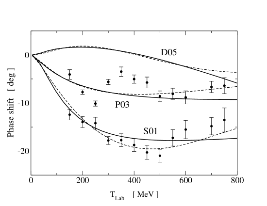
Figure 1: The isospin-zero stretched states phase shifts as function of the $K^{+}$ kinetic energy. The single- and continuous-energy solutions of the GWU analyses are represented with large and small circles. The solid curves represent the phase shifts from the reference potential.

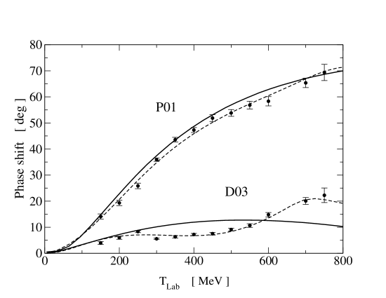
Figure 2: The same as Fig. 1 but for the unstretched states.

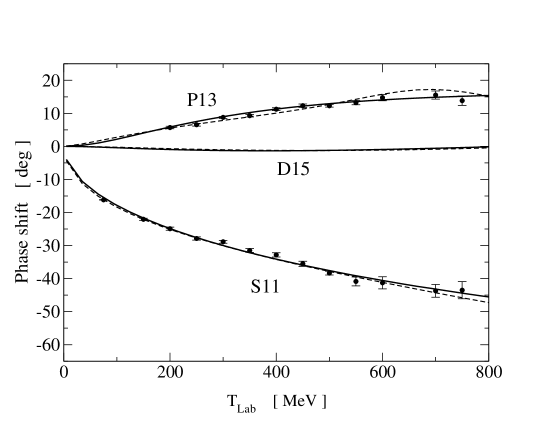
Figure 3: The isospin-one stretched states phase shifts as function of the $K^{+}$ kinetic energy. The single- and continuous-energy solutions of the GWU analyses are represented with large and small circles. The solid curves represent the phase shifts from the reference potential.

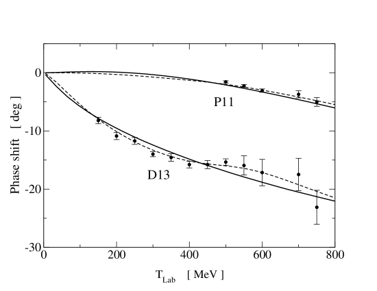
Figure 4: The same as Fig. 3 but for the unstretched states.

Thus, we base the $V_{KN}$ on the current solution of CNS/GWU-KN solutions SAID ; Hyl92 . All used phase shifts, $L\leq 2$, are shown in Figs. 1-4, where we distinguish different data: single (full circles with error bars) and continuous energy (dashed curves) solutions, respectively, and the inversion reference potential phase shifts (solid curves) which reproduce the rational functions of the kinetic energy $T_{\textrm{Lab}}$. The isospin zero (I=0) stretched ($J=L+1/2$) and anti-stretched ($J=L-1/2$) channels are shown in Figs. 1 and 2, respectively. Similarly, the isospin one (I=1) stretched and anti-stretched channels are presented in Figs. 3 and 4, respectively. The corresponding inversion reference potentials are shown in Figs. 5 and 6. In these figures we observe that all potentials are short ranged with significant strengths limited to $r<1$ fm. The very short range behavior depends on the high energy extrapolation of the rational function, which we did as sensible as possible.

The separable potential functions are motivated and tuned to a short range zone in which resonances, inelastic scattering and reactions are supposed to occur Fun01 , viz

$$\phi_{\alpha}(r)=N_{\alpha}r^{L}\exp{[-(r-r_{0})^{2}/a^{2}]},$$ (37)

where we have used $r_{0}=0.5$  fm, $a=0.2$  fm, with $N_{\alpha}$ a normalization constant.

Any identification of resonances and reaction channels is not part of this endeavor. Thus, the separable term strengths $\Gamma_{\alpha}(E)$ are fixed to the continuous energy solution partial wave phase shifts SAID , whose real phase shifts are shown as dashed curves in Figs. 1 to 4. Vanishing imaginary phase shifts are limited to the channels S01, P03, D05 and F07.

III The KA optical potential

An optical model potential (OMP) represents an effective single-particle interaction potential for a projectile caused by the interaction with target nucleons. The underlying many-body problem in Brueckner’s many-body theory yields an OMP in the form of a convolution of a projectile-nucleon effective interaction, the reaction matrix, with the target mixed density.

There are many ways to obtain in practical terms a successful representation of effective interaction and its accurate use in the convolution integral. Here we use the KN $t$-matrix operator, on and off shell, as the effective interaction. Such construction has successfully been used in the past and we recall only its salient features to make the discussion of various results comprehensible. In the projectile-nucleus center of momentum (C.M.) reference frame, the collision of a projectile of kinetic energy $E$ is described by the full-folding OMP, which in a momentum representation is given by Are02

$$U({\bf k}^{\prime},{\bf k};E)=\sum_{N=p,n}\int d{\bf P}\;\rho_{N}({\bf P}+\frac{\bf q}{2}\;,{\bf P}-\frac{\bf q}{2})\;t_{NK^{+}}({\bf k_{r}}^{\prime},{\bf k_{r}};{\bf K}+{\bf P};{s})\;,$$ (38)

where we define the mean momentum ${\bf K}=({\bf k}^{\prime}+{\bf k})/2$ and momentum transfer ${\bf q}={\bf k}^{\prime}-{\bf k}$. Here the effective interaction, in the form of the free scattering $t$ matrix, exhibits an explicit dependence on the relative momenta ${\bf k_{r}}$ and ${\bf k_{r}}^{\prime}$, the total pair momentum ${\bf Q}={\bf K}+{\bf P}$ and the pair $s$ invariant. In particular, the relative momenta take the general form

$${\bf k_{r}}=W{\bf k}-(1-W){\bf p}\;,\qquad{\bf k_{r}}^{\prime}=W^{\prime}{\bf k}^{\prime}-(1-W^{\prime}){\bf p}^{\prime}\;,$$ (39)

where $W$ and $W^{\prime}$ are scalar functions of the momenta of the colliding particles with relativistic kinematics built in Are02 .

The momentum integral $\int d{\bf P}$ signals the folding integral. The intricate dependence of the many vector valued momenta makes the convolution quite complicated and thus the name full-folding approach was coined in order to signal use of the full expression, as compared to much simpler approximated expressions. Physically, the folding integral accounts for dynamical effects due to the Fermi motion as modulated by the shape of target mixed density. For practical reasons we represent the mixed density in terms of the local density $\rho(R)$ via the Slater approximation Are90b , i.e.

$$\rho({\bf P}+\frac{\bf q}{2}\;,{\bf P}-\frac{\bf q}{2})=\frac{1}{\pi^{2}}\int_{0}^{\infty}R^{2}\,dR\,j_{0}(qR)\Theta\left[\hat{k}(R)-P\right]$$ (40)

with $\hat{k}(R)=\left[3\pi^{2}\,\rho(R)\right]^{1/3}$.

The model equation for the $t$ matrix in terms of a reference KN potential in the $K^{+}$N C.M. reference frame takes the form of the Lippmann-Schwinger type (c.f. Eq. 17), i.e.

$$t_{KN}({\bf p}^{\prime},{\bf p};{s})=V_{KN}({\bf p}^{\prime},{\bf p})+2\mu\int\frac{d^{3}k}{(2\pi)^{3}}\frac{V_{KN}({\bf p}^{\prime},{\bf k})\;t_{KN}({\bf k},{\bf p};{s})}{k_{\circ}^{2}+i\varepsilon-k^{2}}.$$ (41)

Here, the energy invariant ${s}$ and associated on-shell momentum $k_{\circ}$ are determined from $s=(m_{K}+\epsilon_{K}+m_{N}+\bar{\epsilon}_{N})^{2}-{\bf Q}^{2}$, where $E$ is the kinetic energy in the KA C.M. frame, $\bar{\epsilon}$ an average binding energy of the target nucleons and ${\bf Q}$ the total pair momentum. The potential $V_{KN}$ is constructed following the inversion procedure described in the previous Section. The calculation of the $t$ matrix on and off shell at various energies follows standard numerical procedures. In the boost of the $t$ matrix from the C.M. to the laboratory reference frame we have included the corresponding Jacobian (or Møller factor) Are02 .

Although full-folding OMP were developed in the eighties for pion as well as nucleon scattering, most $K^{+}$-nucleus scattering analyses continue being made within an on-shell $t\rho$ approximation. We select and discuss three of these factorized forms in this study.

Off-shell $t\rho$.

A first reduction to a $t\rho$ form emerges after setting ${\bf P}=0$ in the $t$ matrix in Eq. (38), thus allowing the integration of the mixed density over the momentum ${\bf P}$. Hence,

$$U({\bf k}^{\prime},{\bf k};E)=\sum_{N=p,n}\rho_{N}({\bf q})\;t_{NK^{+}}({\bf k_{r}}^{\prime},{\bf k_{r}};{\bf K};{s})\;,$$ (42)

where $\rho_{N}({\bf q})$ represents nuclear density in momentum space. In this factorized form the relative momenta ${\bf k_{r}}$ and ${\bf k_{r}}^{\prime}$ lie generally off shell, as no constraints on ${\bf k}$ nor ${\bf k}^{\prime}$ are in place. This reduction is referred as off-shell $t\rho$ approximation and has been extensively applied in nucleon-nucleus scattering. An additional step further can be taken to force the $t$ matrix on shell. Quite generally, features at the $t$-matrix level dictated by four independent variables (two magnitudes, angle and energy) are specified by two of its arguments, one angle and one energy. We have found that on-shell $t\rho$ results for $K^{+}A$ scattering depend, albeit moderately, on the prescription used and we focus on two of them.

On-shell $t\rho$ of the $s-$type.

This is the usual form of the on-shell $t\rho$ approximation and has been applied extensively in hadron-nucleus collisions. We have named it of the $s-$type since it privileges the energy argument in the $t$ matrix. Basically, the energy $\sqrt{s}$ of the $K^{+}N$ pair is determined in the Breit frame with the subsequent determination, on-shell, of the relative momenta. Details can be found in Ref. Pae81 .

On-shell $t\rho$ of the $k-$type.

An alternative prescription, which we refer as of the $k-$type, emerges naturally after considering a series expansion of $U({\bf k},{\bf k^{\prime}})$ in terms of the magnitudes $k$ and $k^{\prime}$ around the on-shell momentum $k_{A}$ in the projectile-nucleus C.M. Then, to lowest order we get

$$U({\bf k^{\prime}},{\bf k})\approx U(k_{A}{\bf\hat{k}^{\prime}},k_{A}{\bf\hat{k}})\;.$$ (43)

As a result, the two relative momenta in the $t$ matrix (c.f. Eq. (39)) become equal in magnitude. The pair energy $\sqrt{s}$ is obtained on-shell from these relative momenta.

IV Applications and results

We focus our applications on differential and total cross sections at kaon momenta in the range 400-1000 MeV/$c$ considering ⁶Li, ¹²C, ²⁸Si and ⁴⁰Ca targets. The ground-state densities of the first three targets were obtained from the nuclear charge density fit to electron scattering Li71a ; Sic70 ; Li71b . The point densities were obtained by unfolding the electromagnetic size of the proton from the charge density. In these cases we assume neutron densities equal to the proton densities. In the case of ⁴⁰Ca we have used the densities from Ref. Neg70 .

The scattering is analyzed within the full-folding OMP and comparisons are made with off- and on-shell $t\rho$ approximations. Thus, we include in the best possible way the off-shell effects in the effective interaction and switch them partially or fully off in the simpler $t\rho$ OMP.

The KA optical potentials are calculated in momentum space following Ref. Are02 . The KA $S$ matrix and derived quantities linked with observable are obtained by solving an OMP Lippmann-Schwinger equation for any of the specified nonlocal potentials.

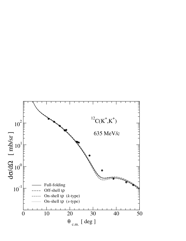
Figure 7: Differential cross section for $K^{+}$+¹²C elastic scattering at P${}_{\textrm{Lab}}$=635 MeV/$c$. The solid curve represents the full-folding results, whereas the long dashed curves corresponds to the off-shell $t\rho$ results. The on-shell $t\rho$ results of the $k$-type and $s$-type are shown with short-dashed and dotted curves, respectively. The data are from Ref. Chr96 .

In Fig. 7 we show the calculated differential cross section for $K^{+}$+¹²C scattering at beam momentum 635 MeV/$c$ with data Chr96 . The solid curves are the full-folding results, whereas the long-dashed curves are the off-shell $t\rho$ results. The on-shell $t\rho$ results of the $s-$type and $k-$type are shown as short-dashed and dotted curves, respectively. Although differences exist among all four results, the differences are quite small. The differences among all $t\rho$ are a measure of the off-shell contributions. The off-shell $t\rho$ result show a uniform shift upward when compared with the full-folding results. More obvious, but still marginal, are differences among the results for scattering angles above $30$ deg.

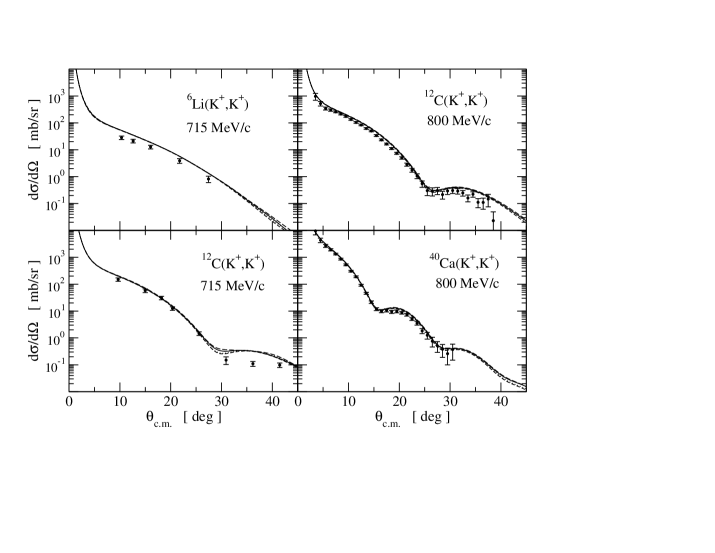
Figure 8: Differential cross section for elastic scattering of $K^{+}$ from ⁶Li (upper-left frame), ¹²C, ⁴⁰Ca (lower right frame) at beam momenta of 715 MeV/$c$ (left frames) and 800 MeV/$c$ (right frames). The curve patterns are the same as in Fig. 7. The data at 715 MeV/$c$ and 800 MeV/$c$ are from Refs. Mic96 and Marl82 , respectively.

Similar applications are shown in Fig. 8, where we present the differential cross section for scattering from ⁶Li, ¹²C and ⁴⁰Ca at beam momenta 715 MeV/$c$ (left frames), and 800 MeV/$c$ (right frames). The data are taken from Mic96 ; Marl82 and the curve textures follows the convention of Fig. 7. Here again we evidence moderate differences among all four approaches, being visible, at best, for angles above $25$  deg. The comparison with data shows for ⁶Li (upper left frame) an overestimation of the theory with respect to the data by a factor of $\sim 1.8$ around 10 degrees. We favour to interpret this discrepancy being caused by uncertainties in the data normalization. The work by Chen et al. Che99 shows that they had a similar problem with ⁶Li. In their study they include a phenomenological second order potential proportional to a power of the nuclear density. They fit the complex strength and power of the density to the data, obtaining results in close resemblance to ours. Overall, the results for ¹²C and ⁴⁰Ca shown in Fig. 8 are in good accord with the data. In the case of ¹²C at 715 MeV/$c$ (lower left frame) some differences between theory and data, at angles above $30$  deg. are there. The full-folding and any of the $t\rho$ approaches are remarkably similar for differential cross sections.

Total cross sections for $K^{+}$-nucleus have been extracted from transmission experiments Kra92 ; Fri97 ; Fri97b . Such data are complementary to the differential cross section data and exhibit often larger differences among the full-folding and $t\rho$ results, even though the same KN effective interaction is used. Before jumping to fast conclusions about the effective interaction or the quality of any of the theoretical models, it is important to remember that the transmission total cross sections $\sigma_{T}$ have their own model dependence built into data. This has been discussed in some detail elsewhere Kau89 ; Ari93 . Using $\sigma_{T}(\Omega)$ as the experimentally measured transmission cross section, subtending a solid angle $\Omega$ from the target along the beam axis, then the total cross section $\sigma_{T}$ is given by

$$\sigma_{T}=\lim_{\Omega\rightarrow 0}\left[\sigma_{T}(\Omega)-\sigma_{C}(\Omega_{>})-\sigma_{CN}(\Omega_{>})\right]+\sigma_{N}(\Omega_{<})+\sigma_{I}(\Omega_{<})\;.$$ (44)

Here $\Omega_{>}$ and $\Omega_{<}$ refers to the integrated cross section outside and inside the solid angle $\Omega$. Furthermore, we use the following nomenclature for particular cross sections: $\sigma_{C}(\Omega_{>})$ for the point charge Coulomb cross section, $\sigma_{CN}(\Omega_{>})$ for the Coulomb and nuclear interaction interference term, $\sigma_{N}(\Omega_{<})$ for the nuclear cross section from the nuclear interaction and $\sigma_{I}(\Omega_{<})$ arising from inelasticities. In the limit $\Omega\rightarrow 0$ the last two terms vanish. However, $\sigma_{CN}$ requires very accurate results for the nuclear plus Coulomb interaction amplitude. This requires knowledge and availability of a high quality optical model in the first place, be as it may be, this introduces a model dependence of $\sigma_{T}$ which is beyond our judgment and puts limits on our conclusions. Nevertheless, we have calculated the total cross sections with all four optical models discussed here and compare the results with data reductions presented in Ref. Fri97 by Friedman et al., and Ref. Fri97b by Friedman, Gal and Mar$\check{\rm e}$s. The difference between the data reported in these two references lies in the way an optical potential, in a $t\rho(r)$ form, is constructed to extract the total cross sections from transition experiments. Whereas in Ref. Fri97 the $t\rho$ form is based on a density independent $t$-matrix strength, in Ref. Fri97b the imaginary part of the strength exhibits a parametric density dependence adjusted to yield, self-consistently, the total cross sections. Thus, the data reported in the second reference is consistent within an empirical medium dependence (c.f. Eq. (5) of Ref. Fri97b ) of the $t$ matrix and reflects, to some extent, the model dependence of their reported measurements.

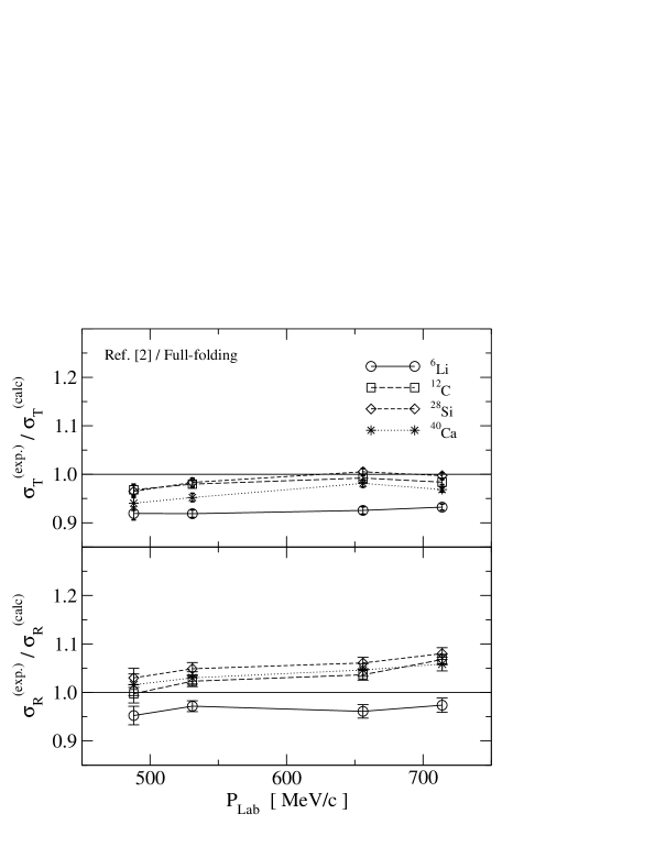
Figure 9: Experimental-to-calculated ratios for the total ($\sigma_{T}$) and reaction ($\sigma_{R}$) cross sections for $K^{+}$ elastic scattering from ⁶Li, ¹²C, ²⁶Si and ⁴⁰Ca, at 488, 531, 656 and 714 MeV/$c$. Results based on the full-folding approach. Connecting lines have been drawn to guide the eye. The data are taken from Ref. Fri97 .

In Figs. 9 and 10 we present the ratios experiment/calculated of the reaction cross sections $\sigma_{R}\mbox{({Exp.})}/\sigma_{R}\mbox{({Calc.})}$ and the total cross sections $\sigma_{T}\mbox{({Exp.})}/\sigma_{T}\mbox{({Calc.})}$ for four target nuclei at four projectile momenta. We notice that all ratios are nearly constant as function of projectile momentum, whereas only the ⁶Li results lie somewhat below the other three cases. Quite similar results are obtained considering the other three forms of the $t\rho$ model. When comparing Figs. 9 and 10 we observe a clear shift in the reaction cross section of the latter with respect to the former. This shift is consistent with the rescaling of the imaginary part of the strength of the $t$ matrix used in the construction of the optical potential Fri97b . The question is, therefore, whether this prescription to incorporate medium corrections effectively accounts for genuine medium effects in the form of short range correlations, Fermi motion and their implied non local effects in the $K^{+}$-nucleus coupling. An assessment of these issues remains to be seen.

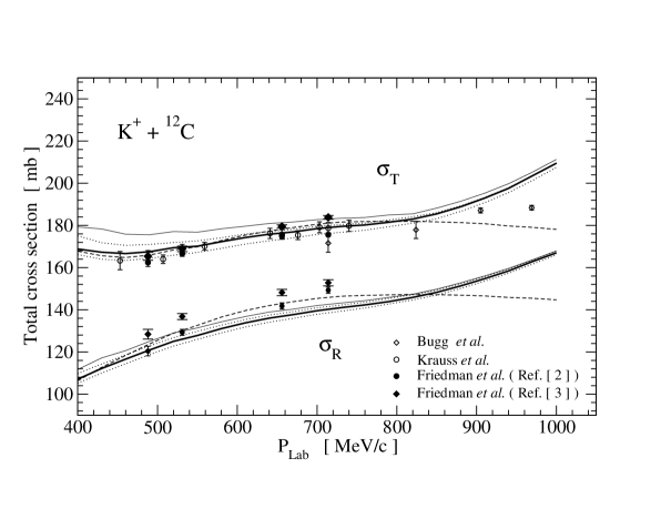
Figure 11: Measured and calculated total cross sections as functions of the beam momentum for $K^{+}$ + ¹²C scattering. The thick curves represent full-folding results; the dotted and thinner solid curves correspond to on- and off-shell $t\rho$ results, respectively. The dashed curves represent full-folding results with the separable strength of the elemental $K^{+}N$ potential suppressed. The data are from Refs. Fri97 ; Fri97b ; Kra92 ; Bug68

The features observed above can also be seen in the Table 1, where we present the measured and calculated cross sections at four momenta for the selected targets, from calculations based on the four approaches discussed here. For instance, the results shown in Fig. 9 correspond to the ratios between the first two blocks of this Table. When comparing the full-folding cross sections with the on-shell $t\rho$ results, we observe that the former lies systematically above the $k-$type, but below the $s-$type. These differences may be used to estimate the off-shell sensitivity, which we estimate $\pm$3% for the worst case. The off-shell $t\rho$ results is always above the other three results and its difference to the data is the largest. These features become more evident in Fig. 11, where we present the measured and calculated reaction $\sigma_{R}$ and total $\sigma_{T}$ cross sections for ¹²C as function of the kaon momentum, in the range 400-1000 MeV/$c$. The data from Bugg et al. Bug68 and Krauss et al. Kra92 are shown with open diamonds and circles, respectively. The data form Friedman et al. Fri97 , and Friedman, Gal and Mar$\check{\rm e}$s Fri97b are shown with black circles and diamonds, respectively. Here, the thicker solid curves represent the full-folding results, whereas the dotted ones are based on the on-shell $t\rho$ approaches. The off-shell $t\rho$ results are shown with the thinner solid curves. Finally, we consider of interest to present full-folding results when only the reference inversion potentials are used in the KN effective interaction, being the separable contribution completely suppressed. These results for $\sigma_{T}$ and $\sigma_{R}$ are shown with dashed curves.

The full-folding and $t\rho$ approaches give an overall consistent agreement with the measured total cross sections up to 900 MeV/$c$, above which they depart from the data. Notice that a nearly full agreement -within error bars- is achieved with the data of Krauss et al. Kra92 . Furthermore, the $s-$type $t\rho$ $\sigma_{T}$ results (upper dotted curves) are in less good agreement with the data in comparison with the $k-$type $t\rho$ and full-folding approach, particularly below 500 MeV/$c$. This illustrates the relevance of the target nucleon Fermi motion in the off-shell $t\rho$ results below $\sim$700 MeV/$c$, shown as thin solid curves, which lies distinctively above the data. A drifting apart of all curves at the lower momenta supports the proper inclusion of Fermi motion in the treatment of the effective interaction.

A closer scrutiny of the gradual departure of the calculated total cross section relative to the data, above 900 MeV/$c$, would require the study of possible uncertainties in the elemental $K^{+}N$ amplitude and to assess their impact on total cross sections. These considerations go beyond the focus of the present work. Incidentally, the results where separable strength of $V_{KN}$ is suppressed (dashed curves) indicate that, despite marginal differences in the description of the real phase shifts, the absorptive component becomes important in the asymptotic behavior of the cross sections. It is in this high-energy regime where the single- and continuous-energy solutions exhibit sizeable differences.

The sensitivity of $\sigma_{T}$ to the alternative approaches considered here is somewhat diminished in the context of the reaction cross section, where all curves stay much closer to each other. An interesting feature which emerges after comparing the calculated total and reaction cross sections is their nearly constant difference above 600 MeV/$c$. In the particular case of ¹²C we observe

$$\sigma_{T}\approx\sigma_{R}+\textrm{39 [mb]}.$$ (45)

A similar behavior is exhibited by the other targets, as inferred from Table 1.

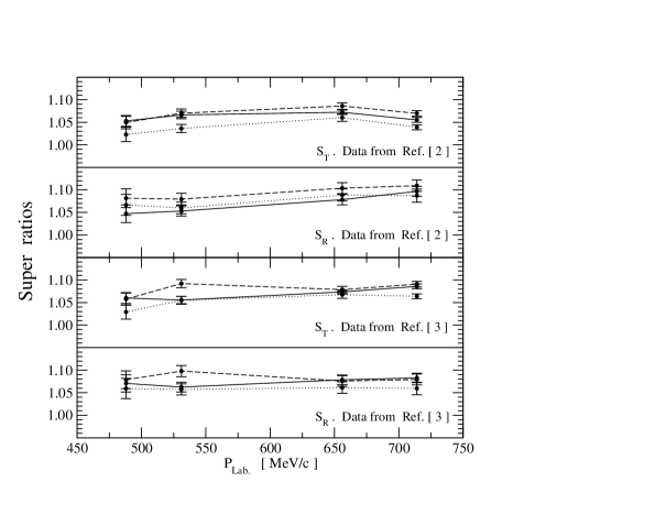
Figure 12: Super ratios for total and reaction cross sections based on data from Refs. Fri97 ; Fri97b and the full-folding approach. The solid, dashed and dotted curves represent results for ¹²C, ²⁸Si and ⁴⁰Ca, respectively.

The study of total cross sections for $N=Z$ nuclei have also been of some interest as a means to gauge the role of medium effects in the propagation of kaons through the nucleus. Weiss and collaborators Wei94 found that the ratio $\sigma_{T}/A$ for ⁶Li and deuterium are nearly the same, suggesting that multiple steps contributions are rather weak in these light targets. Such is not the case for the heavier targets. In order to quantify this feature, Friedman et al. have introduced the super ratios, i.e. the ratio $\sigma_{\textrm{Exp.}}(A)\sigma_{\textrm{Calc.}}(^{6}\textrm{Li})/\sigma_{\textrm{Calc.}}(A)\sigma_{\textrm{Exp.}}(^{6}\textrm{Li})$. Although it is correct that this quantity would diminish normalization uncertainties, its departure from one may not only indicate medium effects but also the level of disagreement between theory and experiment. Indeed, their reported values for each target exhibit distinctive curves as function of the momentum, with values ranging between 1.15 and 1.25. Although limited by the fact that the optical model used to extract the data in Refs. Fri97 ; Fri97b differs from the full-folding model used here, we have also calculated the super ratios using the results in Table I. In Fig. 12 we plot the total ($S_{T}$) and reaction ($S_{R}$) super ratios considering the data from Ref. Fri97 (upper two frames) and Ref. Fri97b (lower two frames), against the full-folding results. Notice that all super ratios are nearly constant as functions of the momentum, with variations between 1.0 and 1.1, consistent with the level of agreement shown in Figs. 9 and 10. Nonetheless, definite analyses of these super ratios requires the use of full-folding $K^{+}A$ optical potentials to extract the cross section data from transmission experiments, an endeavor beyond the scope this work.

V Conclusions

We have studied $K^{+}$-nucleus elastic scattering from light nuclei in the momentum range 400-1000 MeV/$c$ within the full-folding optical model potential framework. To this purpose we have used the $t$ matrix based on a $K^{+}N$ potential model with absolute match of the phase shift analyses reported by the GWU group. The emphasis here has been placed on a strict connection between the bare $K^{+}N$ potential -consistent with the current phase shift analysis- and the $K^{+}$-nucleus scattering process. This feature is achieved by adding a separable term to a local reference potential obtained within the Gel’fand-Levitan-Marchenko quantum inversion. The $t$ matrix, based on this bare potential model, is convoluted with the nuclear mixed density leading to a nonlocal $K^{+}A$ optical potential. The scattering observable were compared with those obtained within off-shell and two alternative versions of on-shell $t\rho$ approximations, which we have named of the $s-$ and $k-$type, respectively. Considering the differential cross-sections, we observe moderate differences among the calculated results from all four approaches. However, reaction and total cross-sections for transmission experiments show a clear sensitivity to the way the Fermi motion is treated, being this more notorious at the lower momenta, i.e. P${}_{\textrm{Lab}}\lesssim$ 600 MeV/$c$. Furthermore, an excellent account of the total cross sections reported by Krauss et al. Kra92 is provided by the full-folding approach for momenta between 450 MeV/$c$ $\lesssim$ P${}_{\textrm{Lab}}\lesssim$ 750 MeV/$c$. These results demonstrate that definite conclusions about the ability of any microscopic approach to describe total cross section data must include the genuine off-shell behavior of the effective interaction and its energy dependence. These conventional medium effects become essential before any conclusive assessment about the manifestation of subhadronic degrees of freedom in KA collisions, particularly a possible manifestation of $\Theta^{+}$(1540) in the collision of $K^{+}$ with nuclei Gal05 .

Table 1: Experimental and calculated reaction and total cross sections (in mb) for $K^{+}$-nucleus scattering at the specified momenta. The data in the first and second block are from Refs. Fri97 ; Fri97b and their corresponding errors are quoted between parentheses.

		Reaction					Total
Source	P${}_{\textrm{Lab}}$
	[MeV/$c$]	6Li	12C	28Si	40Ca		6Li	12C	28Si	40Ca
Data Fri97	488	65.0(1.3)	120.4(2.3)	265.5(5.1)	349.9(7.7)		76.6(1.1)	162.4(1.9)	366.5(4.8)	494.4(7.7)
	531	69.8(0.8)	129.3(1.4)	280.4(3.4)	367.1(4.5)		78.8(0.7)	166.6(1.3)	374.8(3.3)	500.2(4.4)
	656	75.6(1.1)	141.8(1.5)	306.1(3.4)	401.1(5.0)		84.3(0.7)	174.9(0.8)	396.1(2.7)	531.9(4.2)
	714	79.3(1.2)	149.3(1.5)	317.5(3.6)	412.9(5.5)		87.0(0.6)	175.6(0.9)	396.5(2.3)	528.4(2.8)
Data Fri97b	488	67.8(1.3)	128.4(2.3)	276.2(5.1)	362.5(7.7)		77.5(1.1)	165.4(1.9)	373.7(4.8)	503.2(7.7)
	531	73.2(0.8)	136.8(1.4)	299.1(3.4)	384.0(4.5)		80.7(0.7)	168.9(1.3)	391.7(3.3)	521.6(4.4)
	656	79.0(1.1)	148.2(1.5)	311.8(3.4)	408.6(5.0)		86.4(0.7)	179.5(0.8)	403.2(2.7)	548.8(4.2)
	714	82.2(1.2)	152.8(1.5)	320.2(3.6)	417.1(5.5)		88.5(0.6)	183.8(0.9)	411.3(2.3)	550.4(2.8)
Full-folding	488	68.2	120.7	257.7	344.4		83.3	167.7	379.9	525.8
	531	71.8	126.4	267.3	356.4		85.8	170.1	381.2	525.4
	656	78.7	136.8	288.5	383.3		91.1	176.3	394.1	542.0
	714	81.4	139.8	293.9	390.0		93.3	178.5	397.6	545.5
Off-shell $t\rho$	488	70.1	124.8	265.1	353.7		86.3	175.8	396.5	548.4
	531	73.5	129.9	274.0	364.7		88.3	176.9	395.7	545.3
	656	79.9	139.6	293.0	388.7		92.9	181.2	403.2	554.0
	714	83.0	141.9	298.2	395.2		94.7	182.5	405.8	556.3
$t\rho$ $k-$type	488	67.7	118.5	252.4	336.8		82.7	164.4	369.3	508.5
	531	71.2	124.1	262.7	349.8		85.0	166.4	371.6	510.3
	656	78.3	135.0	284.9	378.4		90.5	173.4	386.8	530.8
	714	80.3	138.6	291.3	386.2		92.2	176.3	391.5	535.9
$t\rho$ $s-$type	488	69.2	122.6	260.4	347.4		84.9	170.9	382.9	527.6
	531	72.7	128.0	270.2	359.7		87.0	172.2	383.6	527.0
	656	79.5	138.3	291.1	386.6		92.0	177.6	395.9	543.5
	714	81.4	141.6	297.1	393.8		93.4	180.1	399.7	547.4

Figure 5: The radial dependence of the isospin-zero $K^{+}N$ reference potentials.

Figure 6: The radial dependence of the isospin-one $K^{+}N$ reference potentials.

Figure 10: The same as Fig. 9, but with the data taken from Ref. Fri97b .