The generalised relativistic Lindhard functions

Abstract

We present here analytic expressions for the generalised Lindhard function, also referred to as Fermi Gas polarisation propagator, in a relativistic kinematic framework and in the presence of various resonances and vertices. Particular attention is payed to its real part, since it gives rise to substantial difficulties in the definition of the currents entering the dynamics.

1 Introduction

The linear response theory, whose key ingredient is the Lindhard function (LF), is usually formulated in many-body frameworks like RPA, Landau quasi-particle theory and the like (see, e.g., Ref. [1]). Noteworthy, these simple approaches are often able to describe successfully a quite involved physics.

The LF [2], as originally defined, is just the particle-hole polarisation propagator for a non-relativistic free Fermi gas (FFG) of electrons, and reads

$$\Pi^{0}(q_{0},{|{\bf q}|})=-2i\int\frac{d^{4}p}{(2\pi)^{4}}G_{0}(p+q)G_{0}(p)~{},$$ (1)

where

$$G_{0}(p)=\frac{\theta({|{\bf p}|}-k_{F})}{p_{0}-\dfrac{{|{\bf p}|}^{2}}{2m}+i\eta}+\frac{\theta(k_{F}-{|{\bf p}|})}{p_{0}-\dfrac{{|{\bf p}|}^{2}}{2m}-i\eta}$$ (2)

is the Green’s function of the free electron. The factor 2 in front of (1) comes from the spin traces and is replaced by a factor 4 in nuclear physics (spin plus isospin).

The explicit form of (1) is known since 1954 [2] and, more recently [3, 4], has been expressed according to

$$\Pi^{0}(q_{0},{|{\bf q}|})=2m\left[I[y({|{\bf q}|},q_{0}+i\eta{\rm\ sgn}q_{0}),{|{\bf q}|}]+I[y({|{\bf q}|},-q_{0}-i\eta{\rm\ sgn}q_{0}),{|{\bf q}|}]\right]\;,$$ (3)

where

$$I[y,{|{\bf q}|}]=\frac{1}{(2\pi)^{2}{|{\bf q}|}}\left\{yk_{F}+\frac{1}{2}(y^{2}-k_{F}^{2})\log\frac{y-k_{F}}{y+k_{F}}\right\}~{},$$ (4)

$$y({|{\bf q}|},q_{0})=\frac{mq_{0}}{{|{\bf q}|}}-\frac{{|{\bf q}|}}{2}$$ (5)

being the West’s scaling variable [5]. The analytic extension when the arguments of the logarithms become negative is prescribed to be

$$\log(x\pm i\eta)=\log|x|\pm i\pi\theta(-x)$$ (6)

and the imaginary part of the LF, namely the response to a scalar(-isoscalar) probe, is thus obtained.

Actually many calculations of a fermionic relativistic response function are available — and hence a number of relativistic many-body computations have been performed. Still the need of analytic expressions for the relativistic generalisation of the LF, as an useful input for a variety of calculations, is felt: indeed the results presently available (see, e.g., Ref. [6], which completes a previous result [7], and Ref. [8]) mostly refer to the electroweak case. However we are also interested to the relativistic response to pions and $\rho$-mesons, which lead to different generalisations of the LF. Further, the excitation of nucleonic resonances need to be accounted for and, last but not least, in the quark-gluon plasma the case of massless particles (or one massive — an $s$ or a $c$ quark — and one massless) deserves some attention.

In this paper we address a number of the above cases, showing that they can be handled algebraically in terms of only a few explicit functions.

The scope we pursue is to provide, as a hopefully useful tool for people involved in the field, a rather comprehensive description of the generalised LF in the relativistic case for nucleons and for 1/2 and 3/2 spin resonances. The limiting case quoted above will also be examined in detail.

2 Setting the problem

The channel dependence of the FFG polarisation propagator in a relativistic framework is more pronounced than in the non-relativistic case. We start with the generalised LF for a non interacting nucleonic system

$$\Pi^{0}_{xy}({|{\bf q}|},q_{0})=-i{\rm Tr}\int\frac{d^{4}p}{(2\pi)^{4}}S_{m}(p+q){\cal O}^{x}S_{m}(p){\cal O}^{y}~{},$$ (7)

where

$$\begin{split}S_{m}(p)&=\frac{\not\hskip-3.0ptp+m}{2E_{p}}\left\{\frac{\theta(|{\bf p}|-k_{F})}{p_{0}-E_{p}+i\eta}+\frac{\theta(k_{F}-|{\bf p}|)}{p_{0}-E_{p}-i\eta}-\frac{1}{p_{0}+E_{p}-i\eta}\right\}\\ &=(\not\hskip-3.0ptp+m)\mathfrak{S}_{m}(p)\\ &=S_{0}(p)+\frac{\not\hskip-3.0ptp+m}{2E_{p}}2i\pi\delta(p_{0}-E_{p})\theta(k_{F}-|{\bf p}|)\end{split}$$ (8)

is the nucleon [electron, quark…] propagator in the medium, with

$$E_{p}=\sqrt{p^{2}+m^{2}}~{},$$ (9)

the indices $x$ and $y$ label the incoming and outgoing channel (not necessarily coincident) and ${\cal O}^{x}$, ${\cal O}^{y}$ are some combinations of $\gamma$ matrices and momenta embodying the vertices characterising the channels. Moreover, $S_{0}$ is the analogous of $S_{m}$ in the vacuum.

We have also introduced a “reduced” fermion propagator $\mathfrak{S}_{m}(p)$ spoiled of the Dirac matrix structure, its inverse reading

$$\mathfrak{D}(p)=p^{2}-m^{2}~{}.$$ (10)

Although $\Pi^{0}_{xy}$ as given in Eq. (7) is ill-defined since it is expressed by a divergent integral, we will not require renormalisability, since one may also be interested in effective theories. However, a regularisation procedure is needed in order to cancel the divergences. In the case of (7) (one-loop level) the vacuum subtraction is sufficient [9].

Thus, defining the following polynomial in the relativistic invariants $p^{2}$, $p\cdot q$ and $q^{2}$

$$f_{xy}(p,q)={\rm Tr}(\not\hskip-3.0ptp+m){\cal O}^{x}(\not\hskip-3.0ptp+\not\hskip-3.0ptq+m){\cal O}^{y}~{},$$ (11)

$\Pi^{0}_{xy}$ will read

$$\Pi^{0}_{xy}({|{\bf q}|},q_{0})=-i\int\frac{d^{4}p}{(2\pi)^{4}}\left[\mathfrak{S}_{m}(p+q)\mathfrak{S}_{m}(p)-\mathfrak{S}_{0}(p+q)\mathfrak{S}_{0}(p)\right]f_{xy}(p,q)~{},$$ (12)

where $\mathfrak{S}_{0}=(\not\hskip-3.0ptp+m)^{-1}S_{0}$.

The frequency integration in (12) then reduces to the evaluation of the residua in the (say) lower half-plane, because along the half-circle at infinity the $\pm i\eta$ in the denominators become irrelevant and the integrand vanishes. Thus the regularised $\Pi^{0}_{xy}$ is given by

$$\begin{split}\Pi^{0}_{xy}&({|{\bf q}|},q_{0})=\int\frac{d^{3}p}{(2\pi)^{3}}\frac{1}{4E_{p}E_{p+q}}\\ &\times\left\{\frac{\theta(|{\bf p+q}|-k_{F})\theta(k_{F}-|{\bf p}|)}{q_{0}-E_{p+q}+E_{p}+i\eta}f_{xy}(p,q)\bigm{|}_{p_{0}=E_{p+q}-q_{0}}\right.\\ &-\frac{\theta(k_{F}-|{\bf p+q}|)\theta(|{\bf p}|-k_{F})}{q_{0}-E_{p+q}+E_{p}-i\eta}f_{xy}(p,q)\bigm{|}_{p_{0}=E_{p}}\\ &+\frac{\theta(k_{F}-|{\bf p+q}|)}{q_{0}-E_{p+q}-E_{p}+i\eta}f_{xy}(p,q)\bigm{|}_{p_{0}=E_{p+q}-q_{0}}\\ -&\frac{\theta(k_{F}-{|{\bf p}|})}{q_{0}+E_{p+q}+E_{p}-i\eta}f_{xy}(p,q)\bigm{|}_{p_{0}=E_{p}}\\ &+\theta(|{\bf p+q}|-k_{F})\theta(|{\bf p}|-k_{F})\left.\frac{f_{xy}(p,q)\bigm{|}_{p_{0}=E_{p+q}-q_{0}}-f_{xy}(p,q)\bigm{|}_{p_{0}=E_{p}}}{q_{0}-E_{p+q}+E_{p}}\right\}\end{split}$$ (13)

(note that the term in the last line is never singular).

Now in each denominator the factor $\pm i\eta$ can be replaced by $+i\eta{\rm\ sgn}(q_{0})$. In fact the denominators in the first and third term can only vanish when $q_{0}>0$ so here the replacement $i\eta\to i\eta{\rm\ sgn}(q_{0})$ is immaterial, while the second and fourth ones can vanish for $q_{0}<0$ so that the term $-i\eta$ plays the same role of $i\eta{\rm\ sgn}(q_{0})$.

Since, as we shall see, the explicit form of $f_{xy}$ is inessential for the following discussion, we consider the case $f_{xy}(p,q)=1$. Then, with some manipulations of the $\theta$ functions and a change of variable, Eq. (13) simplifies to

$$\begin{split}\Pi^{0}({|{\bf q}|},q_{0})&=\int\frac{d^{3}p}{(2\pi)^{3}}\frac{\theta(k_{F}-|{\bf p}|)}{2E_{p}}\\ &\hskip-20.0pt\Biggl{\{}\frac{1}{(q_{0}+i\eta{\rm\ sgn}(q_{0})+E_{p})^{2}-E_{p+q}^{2}}+\frac{1}{(q_{0}+i\eta{\rm\ sgn}(q_{0})-E_{p})^{2}-E_{p+q}^{2}}\Biggr{\}}~{}.\end{split}$$ (14)

Eq. (14) displays a great advantage from a practical point of view since

1. each term contains only one $\theta$ function, hence the analytic calculation of the integrals is simplified;

2. $\Pi^{0}$ can be evaluated in a region where it is real and then its imaginary part follows by analytic extension by suitably approaching the real axis in the complex plane of $q_{0}$;

3. it is manifestly even in $q_{0}$.

The same procedure led to the form (3) for the non-relativistic LF.

Now consider a $N^{*}$ excitation of mass $M$. In this case the polarisation propagator at the lowest order is built up by two non-coincident Feynman diagrams, namely (the star will always denote quantities involving a resonance or a resonance-hole pair)

$$\Pi^{*}_{xy}({|{\bf q}|},q_{0})=-i\Biggl{[}\int\frac{d^{4}p}{(2\pi)^{4}}\mathfrak{S}^{*}(p+q)\mathfrak{S}_{m}(p)f^{*xy}(p,q)\\ +\int\frac{d^{4}p}{(2\pi)^{4}}\mathfrak{S}^{*}(p-q)\mathfrak{S}_{m}(p)f^{*xy}(p,-q)\Biggr{]}~{},$$ (15)

where

$$\mathfrak{S}^{*}(p)=\left[{p^{2}-M^{2}+i\eta}\right]^{-1}~{}.$$ (16)

For later purposes we also introduce the inverse of $\mathfrak{S}^{*}$, namely

$$\mathfrak{D}^{*}(p)=p^{2}-M^{2}~{}.$$ (17)

The explicit form of $f^{*xy}$ will be specified later.

Clearly, each term in (15) contains only one $\theta$-function because there is no Pauli blocking. Convergence is ensured by vacuum subtraction and, at variance of the nucleon-hole case, Eq. (8) (third line) tells us that $p_{0}$ can be replaced everywhere by $E_{p}$, since $S_{0}$ never contributes.

3 Structure of the Lindhard functions

In this Section we set up the general structure of the relativistic LFs, which will be later evaluated in some specific cases.

Before presenting the detailed calculation, we observe that the Lorentz covariance is broken by the presence of an infinite medium like the FFG, since this naturally selects a privileged frame of reference, namely the one in which the FFG is at rest. Indeed in this system the nuclear matter has zero momentum, while any boost, no matter how small the velocity is, generates a state with infinite momentum.

If we instead consider a system with mass $M$ and finite momentum ${\bf p}$, then any response function $f$ to a probe carrying a four-momentum $q_{\mu}=(q_{0},{\bf q})$ can only depend upon Lorentz scalars, namely $f=f(p^{2}=M^{2},p\cdot q,q^{2})$; however in the $M\to\infty$ limit $p\cdot q=q_{0}\sqrt{p^{2}+M^{2}}-{\bf p\cdot q}\to q_{0}M$, so that the Lorentz covariance is broken since $f$ will depend upon $q_{0}$ and ${\bf q}$ separately.

3.1 The ingredients

Having clarified the functional dependence of the LFs, we now introduce the ingredients needed to their evaluation. We define the functions

$$U^{*[n]}_{rel}(M;{|{\bf q}|},q_{0})=\int\frac{d^{3}p}{(2\pi)^{3}}\frac{E^{n}_{p}}{2E_{p}}\frac{\theta(k_{F}-{|{\bf p}|})}{(p+q)^{2}-M^{2}+i\eta}\Biggm{|}_{p_{0}=E_{p}}~{},$$ (18)

to be computed in the next Section. The quantities of direct physical interest are the even and odd parts (in $q_{0}$) of $U^{*[n]}_{rel}$, namely

$$\Upsilon^{*[n]}_{\pm}(M;{|{\bf q}|},q_{0})=U^{*[n]}_{rel}(M;{|{\bf q}|},q_{0})\pm U^{*[n]}_{rel}(M;{|{\bf q}|},-q_{0})~{}.$$ (19)

We shall consider in the following a variety of functions $f_{xy}$, each one giving rise to its own LF: remarkably these all are expressed in terms of few basic cases. Note that when $f_{xy}=1$ then Eq. (14) becomes

$$\Pi^{0}({|{\bf q}|},q_{0})=\Upsilon^{[0]}_{+}(m;{|{\bf q}|},q_{0}+i{\rm\ sgn}q_{0})~{}.$$ (20)

The above functions display a complex analytic structure (logarithmic cuts) and have a well defined imaginary part and a well defined asymptotic behaviour (in $q_{0}$), namely $\Upsilon^{*[n]}_{\pm}\simeq q_{0}^{-2}$: this means that the real part of $\Upsilon^{*[n]}_{\pm}$, hence of the LF, can be univoquely recovered from its imaginary part via dispersion relations.

However in general $f_{xy}$ is a polynomial in $q_{0}^{2}$. Each term of this polynomial generates contributions to $\Pi^{0}$ with the same imaginary part (up to trivial coefficients), but with different asymptotic behaviour, so that the evaluation of the real part will require subtracted dispersion relations. The subtracted parts will be called contact terms. These can be expressed in terms of the $k_{F}$-dependent function

$$\begin{split}{\mathfrak{T}}^{[0]}=-i\int\frac{d^{4}p}{(2\pi)^{4}}\mathfrak{S}_{m}(p)&\begin{CD}@>{\text{renormalisation}}>{}>\end{CD}\int\frac{d^{3}p}{(2\pi)^{3}}\dfrac{\theta(k_{F}-{|{\bf p}|})}{2E_{p}}\\ &=\frac{1}{8\pi^{2}}\left[k_{F}E_{F}-m^{2}\log\frac{k_{F}+E_{F}}{m}\right]~{},\end{split}$$ (21)

where $E_{F}=\sqrt{k_{F}^{2}+m^{2}}$ and, more generally,

$${\mathfrak{T}}^{[n]}=\int\frac{d^{3}p}{(2\pi)^{3}}\dfrac{\theta(k_{F}-{|{\bf p}|})}{2}E_{p}^{n-1}=\frac{k_{F}^{3}}{12\pi^{2}}m^{n-1}{}_{2}F_{1}\left(\frac{3}{2},\frac{1}{2}-\frac{n}{2};\frac{5}{2};-\frac{k_{F}^{2}}{m^{2}}\right)~{},$$ (22)

where ${}_{2}F_{1}$ is an hypergeometric function.

Note that contact terms are also indirectly related to the renormalizability of a theory, because their presence alter the power counting in a bosonic loop entering in an RPA-dressed bosonic propagator closed on itself or on a fermionic line.

Now we are in a position to deal with the general structure of the LFs. Since we shall consider (pseudo-)scalar and (pseudo-)vector couplings, our LFs will carry 0, 1 or 2 vector indices only. Tensor couplings could bring into play other functions ($U^{*[3]}_{rel}$ and $U^{*[4]}_{rel}$), but they seem not to be, at present, of physical interest.

3.2 Scalar case: 0-index functions

Here ${\cal O}^{x}$ and ${\cal O}^{y}$ have no vector structure, hence $f^{*}_{xy}=f^{*}_{xy}(p^{2},p\cdot q,q^{2})$, in general a polynomial, is a Lorentz scalar. Replacing then $p^{2}$ with $\mathfrak{D}(p)+m^{2}$ and using the identity

$$\begin{split}p\cdot q&=\frac{1}{2}\left[(p+q)^{2}-M^{2}\right]-\frac{1}{2}(p^{2}-m^{2})-\frac{1}{2}\rho q^{2}\\ &=\frac{1}{2}\mathfrak{D}^{*}(p+q)-\frac{1}{2}\mathfrak{D}(p)-\frac{1}{2}\rho q^{2}~{},\end{split}$$ (23)

we can rewrite $f^{*}_{xy}$ in the form

$$f^{*}_{xy}=A_{xy}^{S}(q^{2})+\sum_{mn}\lambda_{mn}^{S}(q^{2})\left\{\mathfrak{D}^{*}(p+q)\right\}^{m}\left\{\mathfrak{D}(p)\right\}^{n}~{},$$ (24)

being $A^{S}(q^{2})$ and $\lambda_{mn}^{S}(q^{2})$’s Lorentz scalars (hence the superscript $S$). In (23) we have introduced, as in [11], the dimensionless quantity

$$\rho=1-\frac{M^{2}-m^{2}}{q^{2}}~{}.$$ (25)

In the case $M=m$ we have $f^{*}_{xy}\to f_{xy}$ and $\rho=1$. Further, in Eq. (24) the summed indices $m$, $n$ must satisfy $m+n\geq 1$.

If we consider the resonance-hole case, we have to insert (24) into (15). Then the first term on the r.h.s. of Eq. (24) yields $A_{xy}^{S}(q^{2})\Upsilon^{*[0]}_{+}(M;{|{\bf q}|},q_{0})$ and the second generates the contact terms, which in the present case can be expressed in terms of the following functions

$$T^{*[m,n]}_{S\pm}({|{\bf q}|},q_{0})=-i\int\frac{d^{4}p}{(2\pi)^{4}}\left\{\mathfrak{D}^{*}(p+q)\right\}^{m-1}\left\{\mathfrak{D}(p)\right\}^{n-1}\\ \mp i\int\frac{d^{4}p}{(2\pi)^{4}}\left\{\mathfrak{D}^{*}(p-q)\right\}^{m-1}\left\{\mathfrak{D}(p)\right\}^{n-1}~{}.$$ (26)

Then, because of the vacuum subtraction, only the $n=0$ term survives in (24) (otherwise any dependence upon $k_{F}$ is lost) and of course it must be $m\geq 1$.

The 3/2-spin resonance generates an additional complication due to the possible presence of projection operators, as discussed in Sec. 8 (see Eq. (99) for details): these will require the addition of a function $B^{S}(q^{2})$, whose role will be clarified later. In conclusion, the most general 0-index LF has the structure

$$\begin{split}\Pi^{*(0)}_{xy}(M;{|{\bf q}|},q_{0})&\equiv\Pi^{*S}_{xy\pm}(M;{|{\bf q}|},q_{0})=A_{xy}^{S}(q^{2})\Upsilon^{*[0]}_{\pm}(M;{|{\bf q}|},q_{0})\\ &+B_{xy}^{S}(q^{2})\Upsilon^{*[0]}_{\pm}(M=0;{|{\bf q}|},q_{0})+\sum_{m\geq 1}\lambda_{m0}^{S}(q^{2})T^{*[m,0]}_{S\pm}({|{\bf q}|},q_{0})\end{split}$$ (27)

with $A_{xy}^{S}(q^{2})$, $B_{xy}^{S}(q^{2})$ and $\lambda_{m0}^{S}(q^{2})$ to be specified according to the problem one deals with (however $B_{xy}^{S}(q^{2})=0$ for spin-1/2 particles).

The functions $T^{*[m,0]}_{S\pm}({|{\bf q}|},q_{0})$, linked to the functions $\mathfrak{T}$ of Eq. (22), are not Lorentz invariant. Those entering our calculations are explicitly given in Appendix A.

The nucleon-hole case is more involved. Eq. (24) still holds valid, provided $\mathfrak{D}^{*}=\mathfrak{D}$, but the subtraction scheme will be different, since $\mathfrak{D}(p+q)$ also depends upon $k_{F}$. Thus the contact terms will also be different because both the cases $m=0,n\not=0$ and $m\not=0,n=0$ contribute in this instance after the vacuum subtraction.

3.3 Vector case: 1-index functions

Vector-like LFs can only arise through the combination of a scalar and a vector vertex. Lorentz invariance would forbid such transitions, because scalar and vectors belong to different representations of the Lorentz group but, since the infinite nuclear medium violates covariance due to the presence of the $\theta$-functions, these terms may occur. Hence in the nuclear medium a vector meson (the $\omega$, for instance) can be converted into a $\sigma$.

By covariance the functions $f_{xy}^{\mu}$ must have the structure

$$f_{xy}^{\mu}=\alpha t^{\mu}+\beta q^{\mu}~{},$$ (28)

where the transverse momentum

$$t^{\mu}=p^{\mu}-\frac{p\cdot q}{q^{2}}q^{\mu}$$ (29)

has been introduced ($t\cdot q=0$). The second term on the r.h.s. of Eq. (28) is immediately handled, since the vector $q^{\mu}$ factors out of the integral and the scheme of the previous subsection applies, but it gives rise to a $\Pi^{*(1)\mu}_{xy}$ which is not gauge invariant.

Instead, the vector-like LF generated by the first term of $f_{xy}^{\mu}$ (to be called $\Pi^{*(1)\mu~{}\rm cons}_{xy}$) obeys the conservation law $q_{\mu}\Pi^{*(1)\mu~{}\rm cons}_{xy}=0$ and can be cast into the form

$$\Pi^{*(1)\mu~{}\rm cons}_{xy}=\Pi^{*(1)0~{}\rm cons}_{xy}\mathfrak{N}^{\mu}~{},$$ (30)

where we have introduced the four-component object (not a vector)

$$\mathfrak{N}^{\mu}=\left(1,\dfrac{q_{0}q^{i}}{{|{\bf q}|}^{2}}\right)~{}.$$ (31)

Hence it is sufficient to compute the 0 component of $\Pi^{*(1)\mu}_{xy}$ only. Defining

$$\mathfrak{Q}^{*V}_{\pm}(M;{|{\bf q}|},q_{0})=-i\int\frac{d^{4}p}{(2\pi)^{4}}t^{0}\left\{\mathfrak{S}^{*}(p+q)\mathfrak{S}_{m}(p)\pm\mathfrak{S}^{*}(p-q)\mathfrak{S}_{m}(p)\right\}$$ (32)

and

$$T^{*[m,n]}_{V\pm}({|{\bf q}|},q_{0})=-i\int\frac{d^{4}p}{(2\pi)^{4}}t^{0}\;\{\mathfrak{D}^{*}(p+q)\}^{m-1}\{\mathfrak{D}(p)\}^{n-1}\pm(q_{0}\leftrightarrow-q_{0})$$ (33)

the 0 component of the vector-like LF, using again (23), takes the form

$$\begin{split}\Pi^{*(1)0~{}\rm cons}_{xy\pm}&\equiv\Pi^{*V}_{xy\pm}=A^{V}_{xy}(q^{2})\mathfrak{Q}^{*V}_{\pm}(M;{|{\bf q}|},q_{0})+B^{V}_{xy}(q^{2})\mathfrak{Q}^{*V}_{\pm}(M=0;{|{\bf q}|},q_{0})\\ &+\sum_{m}\lambda^{V}_{m0}T^{*[m,0]}_{V\pm}({|{\bf q}|},q_{0})~{},\end{split}$$ (34)

where we have accounted for the projection operators (99) and the parity is not specified. Again the functions $A$, $B$ and $\lambda$ have to be specified according to the problem.

The new function $\mathfrak{Q}^{*V}_{\pm}$ is expressible in terms of the $\Upsilon^{*[n]}$ as follows

$$\mathfrak{Q}^{*V}_{\pm}(M;{|{\bf q}|},q_{0})=\Upsilon^{*[1]}_{\pm}(M;{|{\bf q}|},q_{0})+\frac{1}{2}\rho q_{0}\Upsilon^{*[0]}_{\mp}(M;{|{\bf q}|},q_{0})-\begin{cases}0\\ \dfrac{q_{0}}{q^{2}}\mathfrak{T}^{[0]}\end{cases}~{},$$ (35)

while the $T^{*[m,n]}_{V}$ relevant to us are listed in Appendix A. In conclusion the general structure of the 1-index LF reads

$$\Pi^{*(1)\mu}_{xy}(M;{|{\bf q}|},q_{0})=\Pi^{*V}_{xy+}(M;{|{\bf q}|},q_{0})\mathfrak{N}^{\mu}+q^{\mu}\Pi^{*S}_{xy-}(M;{|{\bf q}|},q_{0})~{}.$$ (36)

Again the nucleonic case is more tricky, because we must first replace (32) with

$$\mathfrak{Q}^{V}({|{\bf q}|},q_{0})=-i\int\frac{d^{4}p}{(2\pi)^{4}}t^{0}\mathfrak{S}_{m}(p+q)\mathfrak{S}_{m}(p)~{},$$ (37)

next express $p\cdot q$ according to (23) and finally use directly the expression (13). Following exactly the same path leading to Eq. (14) we obtain the limiting case ($M=m$) of Eq. (35).

3.4 Tensor case: 2-indices functions

The 2-indices functions, which require two vector-type vertices, can be split into a symmetric and antisymmetric part that need to be studied separately.

3.4.1 Symmetric case

In the symmetric case, since $f^{\mu\nu}_{xy}$ is a true tensor, Lorentz covariance imposes the structure

$$f^{\mu\nu}_{xy~{}{\rm symm}}=a_{1}\left(q^{2}g^{\mu\nu}-q^{\mu}q^{\nu}\right)+a_{2}t^{\mu}t^{\nu}+a_{3}(t^{\mu}q^{\nu}+q^{\mu}t^{\nu})+a_{4}q^{\mu}q^{\nu}$$ (38)

the $a_{i}$ being Lorentz invariants.

The first two terms of (38) correspond to a conserved current. Let us denote the associated LF by $\Pi^{*(2)\mu\nu~{}\rm cons}_{xy~{}\rm symm}(M;{|{\bf q}|},q_{0})$, which can be split into a longitudinal ($\Pi^{*L}_{xy}$) and a transverse ($\Pi^{*T}_{xy}$) polarisation propagators, defined according to

$$\Pi^{*L}(M;{|{\bf q}|},q_{0})&=\Pi^{*(2)00~{}\rm cons}_{xy~{}\rm symm}(M;{|{\bf q}|},q_{0})~{},\\ \Pi^{*T}(M;{|{\bf q}|},q_{0})=\left(\delta_{ij}-\frac{q_{i}q_{j}}{{|{\bf q}|}^{2}}\right)\Pi^{*(2)ij~{}\rm cons}_{xy~{}\rm symm}(M;{|{\bf q}|},q_{0})$$ (39)

and, in a compact notation,

$$\Pi^{*(2)\mu\nu~{}\rm cons}_{xy~{}\rm symm}(M;{|{\bf q}|},q_{0})=\\ \left(\begin{tabular}[]{c|c}$\Pi^{*L}$&$\frac{q_{0}q_{i}}{{|{\bf q}|}^{2}}\Pi^{*L}$\\ \hline\cr$\frac{q_{0}q_{j}}{{|{\bf q}|}^{2}}\Pi^{*L}$&$\frac{q_{0}^{2}}{{|{\bf q}|}^{2}}\Pi^{*L}\frac{q_{i}q_{j}}{{|{\bf q}|}^{2}}+\frac{1}{2}\Pi^{*T}\left(\delta_{ij}-\frac{q_{i}q_{j}}{{|{\bf q}|}^{2}}\right)$\end{tabular}\right)~{}.$$ (40)

The first term in the r.h.s. of (38) is easily handled, since it reduces to the 0-index case. The second instead requires the introduction of two new quantities with the associated contact terms. We thus define

$$\mathfrak{Q}^{*L}_{\pm} (M;{|{\bf q}|},q_{0})=\int\frac{d^{3}p}{(2\pi)^{3}}\frac{(t^{0})^{2}}{2E_{p}}\frac{\theta(k_{F}-{|{\bf p}|})}{(p+q)^{2}-M^{2}+i\eta}\Biggm{|}_{p_{0}=E_{p}}\pm~{}(q\longleftrightarrow-q)$$

$$=\Upsilon^{*[2]}_{\pm}(M;{|{\bf q}|},q_{0})+q_{0}\rho\Upsilon^{*[1]}_{\mp}(M;{|{\bf q}|},q_{0})$$

$$+\frac{1}{4}q_{0}^{2}\rho^{2}\Upsilon^{*[0]}_{\pm}(M;{|{\bf q}|},q_{0})-\begin{cases}\dfrac{q_{0}^{2}\rho}{2q^{2}}\mathfrak{T}^{[0]}\\ \dfrac{q_{0}}{q^{2}}\left(1-\frac{{|{\bf q}|}^{2}}{q^{2}}\right)\mathfrak{T}^{[1]}\end{cases}$$ (41)

and

$$\mathfrak{Q}^{*T}_{\pm} (M;{|{\bf q}|},q_{0})$$

$$=\frac{1}{{|{\bf q}|}^{2}}\int\frac{d^{3}p}{(2\pi)^{3}}\frac{{|{\bf p}|}^{2}{|{\bf q}|}^{2}-({\bf p}\cdot{\bf q})^{2}}{2E_{p}}\frac{\theta(k_{F}-{|{\bf p}|})}{(p+q)^{2}-M^{2}+i\eta}\Biggm{|}_{p_{0}=E_{p}}$$

$$\pm~{}(q\longleftrightarrow-q)$$

$$=-\frac{q^{2}}{{|{\bf q}|}^{2}}\Biggl{\{}\Upsilon^{*[2]}_{\pm}(M;{|{\bf q}|},q_{0})+q_{0}\rho\Upsilon^{*[1]}_{\mp}(M;{|{\bf q}|},q_{0})$$

$$+\left(\frac{1}{4}q^{2}\rho^{2}+\frac{m^{2}{|{\bf q}|}^{2}}{q^{2}}\right)\Upsilon^{*[0]}_{\pm}(M;{|{\bf q}|},q_{0})\Biggr{\}}+\begin{cases}\dfrac{q^{2}\rho}{2{|{\bf q}|}^{2}}\mathfrak{T}^{[0]}\\ ~{}\\ \dfrac{q_{0}}{q^{2}}{\mathfrak{T}}^{[1]}\end{cases}$$ (42)

together with the contact terms

$$T^{*[m,n]}_{L\pm}({|{\bf q}|},q_{0}) =-i\int\frac{d^{4}p}{(2\pi)^{4}}(t^{0})^{2}\;\{\mathfrak{D}^{*}(p+q)\}^{m-1}\{\mathfrak{D}(p)\}^{n-1}\pm(q_{0}\leftrightarrow-q_{0})$$ (43)

and

$$T^{*[m,n]}_{T\pm}({|{\bf q}|},q_{0}) =\frac{-i}{{|{\bf q}|}^{2}}\int\frac{d^{4}p}{(2\pi)^{4}}\left[{|{\bf p}|}^{2}{|{\bf q}|}^{2}-({\bf p}\cdot{\bf q})^{2}\right]\times$$ (44)

$$\{\mathfrak{D}^{*}(p+q)\}^{m-1}\{\mathfrak{D}(p)\}^{n-1}\pm(q_{0}\leftrightarrow-q_{0})~{}.$$

Thus, applying (23) and (27), we obtain

$$\Pi^{*L}_{xy}(M;{|{\bf q}|},q_{0}) =-{|{\bf q}|}^{2}\Pi^{*S}_{xy}(M;{|{\bf q}|},q_{0})+A^{LT}_{xy}(q^{2})\mathfrak{Q}^{*L}_{+}(M;{|{\bf q}|},q_{0})$$ (45)

$$+B^{LT}_{xy}(q^{2})\mathfrak{Q}^{*L}_{+}(M=0;{|{\bf q}|},q_{0})+\sum_{m}\lambda_{m0}^{LT}(q^{2})T^{*[m,0]}_{L+}({|{\bf q}|},q_{0})$$

$$\Pi^{*T}_{xy}(M;{|{\bf q}|},q_{0}) =-2q^{2}\Pi^{*S}_{xy}(M;{|{\bf q}|},q_{0})+A^{LT}_{xy}(q^{2})\mathfrak{Q}^{*T}_{+}(M;{|{\bf q}|},q_{0})$$ (46)

$$+B^{LT}_{xy}(q^{2})\mathfrak{Q}^{*T}_{+}(M=0;{|{\bf q}|},q_{0})+\sum_{m}\lambda_{m0}^{LT}(q^{2})T^{*[m,0]}_{T+}({|{\bf q}|},q_{0})$$

(note that the same coefficients $A^{LT}$, $B^{LT}$ and $\lambda^{LT}$ enter in both $\Pi^{*L}$ and $\Pi^{*T}$). The above relations give the structure of the longitudinal and transverse LFs and thus fully describe $\Pi^{*(2)\mu\nu~{}\rm cons}_{xy~{}\rm symm}$ through (40). Finally, the remaining terms of (38) can be reduced to simpler cases and one gets the final result

$$\begin{split}\Pi^{*(2)\mu\nu}_{xy~{}\rm symm}(M;{|{\bf q}|},q_{0})&=\Pi^{*(2)\mu\nu~{}\rm cons}_{xy~{}\rm symm}(M;{|{\bf q}|},q_{0})\\ &+(q^{\mu}\mathfrak{N}^{\nu}+q^{\nu}\mathfrak{N}^{\mu})\Pi^{*V}_{xy-}(M;{|{\bf q}|},q_{0})\\ &+q^{\mu}q^{\nu}\tilde{\Pi}^{*S}_{xy+}(M;{|{\bf q}|},q_{0})~{}.\end{split}$$ (47)

The last term on the r.h.s. of (47), namely $\tilde{\Pi}^{*S}_{xy+}$, corresponds to a LF with the same structure of $\Pi^{*S}_{xy+}$ but with different ingredients: these will be called $\tilde{A}^{S}$, $\tilde{B}^{S}$ and $\tilde{\lambda}^{S}_{m0}$, respectively, to avoid confusion.

Again the nucleon-hole case must be handled separately, by using the analogous of Eq. (37). Clearly now, at variance of the resonance case, only the $\mathfrak{Q}^{*L,T}_{+}$ terms exist, and a straightforward calculation shows that Eqs. (41) and (42) still hold valid.

3.4.2 Antisymmetric case

An antisymmetric tensor should have the form

$$f^{*\mu\nu}_{xy~{}\rm antisymm}=b_{1}(t^{\mu}q^{\nu}-q^{\mu}t^{\nu})+b_{2}\epsilon^{\mu\nu\lambda\rho}p_{\lambda}q_{\rho}$$ (48)

and the general structure of $\Pi^{*(2)\mu\nu}_{xy~{}\rm antisymm}$ will accordingly be

$$\Pi^{*(2)\mu\nu}_{xy~{}\rm antisymm}(M;{|{\bf q}|},q_{0})=(q^{\mu}\mathfrak{N}^{\nu}-q^{\nu}\mathfrak{N}^{\mu})\Pi^{*V}_{xy-}(M;{|{\bf q}|},q_{0})\\ +q_{\lambda}\mathfrak{N}^{\sigma}g_{\sigma\rho}\epsilon^{\mu\nu\rho\lambda}\tilde{\Pi}^{*V}_{xy-}(M;{|{\bf q}|},q_{0})~{}.$$ (49)

Again the function $\tilde{\Pi}^{*V}_{xy-}$ entering the above has the same structure given by Eq. (34), but with the functions $A^{V}$, $B^{V}$ and $\lambda^{V}_{m0}$ replaced by $\tilde{A}^{V}$, $\tilde{B}^{V}$ and $\tilde{\lambda}^{V}_{m0}$.

4 Analytic evaluation of $U^{*[0]}_{rel}(M;{|{\bf q}|},q_{0})$

In this section we explicitly compute the function $U^{*[0]}_{rel}$ defined by Eq. (18) (the other two functions $U^{*[1]}_{rel}$ and $U^{*[2]}_{rel}$ can be obtained along the same path and the results are reported in Appendix B).

Assuming here $\Im~{}q_{0}\not=0$ we get

$$\begin{split}U^{*[0]}_{rel}&=\int\frac{d^{3}p}{(2\pi)^{3}}\frac{1}{2E_{p}}\frac{\theta(k_{F}-{|{\bf p}|})}{2E_{p}q_{0}-2{\bf p}\cdot{\bf q}+q^{2}\rho}\\ &=\frac{1}{16\pi^{2}{|{\bf q}|}}\int\limits_{0}^{k_{F}}\frac{p\,dp}{E_{p}}\log\frac{q^{2}\rho+2p{|{\bf q}|}+2q_{0}E_{p}}{q^{2}\rho-2p{|{\bf q}|}+2q_{0}E_{p}}~{}.\end{split}$$ (50)

Note that the dependence upon $M$ is fully embodied in the inelasticity parameter $\rho$. Integration by parts yields

$$\begin{split}U^{*[0]}_{rel}&=\frac{1}{16\pi^{2}{|{\bf q}|}}E_{F}\log\frac{q^{2}\rho+2k_{F}{|{\bf q}|}+2E_{F}q_{0}}{q^{2}\rho-2k_{F}{|{\bf q}|}+2E_{F}q_{0}}\\ &-\frac{1}{4\pi^{2}}\int\limits_{0}^{k_{F}}dp\;\frac{q^{2}\rho E_{p}+2m^{2}q_{0}}{\left(q^{2}\rho-2p{|{\bf q}|}+2E_{p}q_{0}\right)\left(q^{2}\rho+2p{|{\bf q}|}+2E_{p}q_{0}\right)}~{}.\end{split}$$ (51)

The integrand in (51) displays four poles, located at $p=\pm y^{*}_{\pm}$. Defining

$$Q_{\pm}=(M\pm m)^{2}-q^{2}$$ (52)

and

$$\Delta^{*}=\sqrt{\rho^{2}-\frac{4m^{2}}{q^{2}}}=-\frac{\sqrt{Q_{+}Q_{-}}}{q^{2}}=-\frac{\sqrt{\left[(M-m)^{2}-q^{2}\right]\left[(M+m)^{2}-q^{2}\right]}}{q^{2}}$$ (53)

(with the chosen sign $\Delta^{*}$ is positive in the space-like region) we obtain for the poles the expression

$$y_{\pm}^{*}=\frac{{|{\bf q}|}}{2}\rho\pm\frac{q_{0}}{2}\Delta^{*}~{}.$$ (54)

The $\pm y^{*}_{\pm}$ are the branch points defining the region where, for real $q_{0}$, (51) develops an imaginary part. In particular the lowest positive branch point is just the lowest possible longitudinal momentum for the occurrence of a resonance-hole pair and consequently coincides (up to a sign) with the $y$ scaling variable. Indeed $-y^{*}_{-}$, taken at $M=m$, is just the $y$ scaling variable for the relativistic Fermi gas [10].

The integrand of (51) can be split according to

$$\frac{E_{p}}{32\pi^{2}{|{\bf q}|}}\left\{\frac{1}{p+y^{*}_{-}}+\frac{1}{p+y^{*}_{+}}-\frac{1}{p-y^{*}_{-}}-\frac{1}{p-y^{*}_{+}}\right\}\\ +\frac{1}{32\pi^{2}{|{\bf q}|}}\left\{\frac{R^{*}_{-}}{p+y^{*}_{-}}-\frac{R^{*}_{+}}{p+y^{*}_{+}}-\frac{R^{*}_{-}}{p-y^{*}_{-}}+\frac{R^{*}_{+}}{p-y^{*}_{+}}\right\}~{},$$ (55)

where

$$R_{\pm}^{*}=\frac{{|{\bf q}|}}{2}\Delta^{*}\pm\frac{q_{0}}{2}\rho$$ (56)

has the property

$$(R_{\pm}^{*})^{2}=m^{2}+(y_{\pm}^{*})^{2}$$ (57)

and is trivially linked to the scaling variable $\psi^{*}$ used in Refs. [11, 12, 13, 14] by

$$R^{*}_{-}=m+(E_{F}-m){\psi^{*}}^{2}~{}.$$ (58)

We can now easily compute explicitly (51), getting

$$\begin{split}&U^{*[0]}_{rel}(M;{|{\bf q}|},q_{0})=-\frac{\rho}{(4\pi)^{2}}\log\frac{k_{F}+E_{F}}{m}\\ &-\frac{E_{F}}{16\pi^{2}{|{\bf q}|}}\log\frac{q^{2}\rho-2k_{F}{|{\bf q}|}+2E_{F}q_{0}}{q^{2}\rho+2k_{F}{|{\bf q}|}+2E_{F}q_{0}}\\ &+\frac{q_{0}\rho}{64\pi^{2}{|{\bf q}|}}\log\frac{(k_{F}-y_{-}^{*})^{2}(m^{2}+k_{F}y_{+}^{*}+E_{F}R^{*}_{+})(m^{2}-k_{F}y_{+}^{*}-E_{F}R^{*}_{+})}{(k_{F}+y_{+}^{*})^{2}(m^{2}+k_{F}y_{-}^{*}+E_{F}R^{*}_{-})(m^{2}-k_{F}y_{-}^{*}-E_{F}R^{*}_{-})}\\ &-\frac{\Delta^{*}}{64\pi^{2}}\log\frac{m^{4}(k_{F}-y_{-}^{*})^{2}(k_{F}+y_{+}^{*})^{2}}{\left[m^{4}-(k_{F}y^{*}_{-}+E_{F}R^{*}_{-})^{2}\right]\left[m^{4}-(k_{F}y^{*}_{+}+E_{F}R^{*}_{+})^{2}\right]}\end{split}$$ (59)

or, with some algebra,

$$\begin{split}&U^{*[0]}_{rel}(M;{|{\bf q}|},q_{0})=-\frac{y^{*}_{-}+y^{*}_{+}}{16\pi^{2}{|{\bf q}|}}\log\frac{k_{F}+E_{F}}{m}+\frac{R^{*}_{+}-R^{*}_{-}+2E_{F}}{64\pi^{2}{|{\bf q}|}}\times\\ &\times\log\frac{(k_{F}-y_{-}^{*})^{2}(m^{2}+k_{F}y_{+}^{*}+E_{F}R^{*}_{+})(m^{2}-k_{F}y_{+}^{*}-E_{F}R^{*}_{+})}{(k_{F}+y_{+}^{*})^{2}(m^{2}+k_{F}y_{-}^{*}+E_{F}R^{*}_{-})(m^{2}-k_{F}y_{+}^{*}-E_{F}R^{*}_{+})}\\ &-\frac{R^{*}_{+}+R^{*}_{-}}{64\pi^{2}{|{\bf q}|}}\log\frac{m^{4}(k_{F}-y_{-}^{*})^{2}(k_{F}+y_{+}^{*})^{2}}{\left[m^{4}-(k_{F}y^{*}_{-}+E_{F}R^{*}_{-})^{2}\right]\left[m^{4}-(k_{F}y^{*}_{+}+E_{F}R^{*}_{+})^{2}\right]}~{},\end{split}$$ (60)

which depends, but for the overall factor ${|{\bf q}|}^{-1}$, only upon the two scaling variables $y^{*}_{\pm}$.

Finally, with $E^{*}_{p}=\sqrt{M^{2}+p^{2}}$ (hence $E^{*}_{k_{F}\pm q}=\sqrt{M^{2}+(k_{F}\pm q)^{2}}$) and bringing back $q_{0}$ to the real axis, Eq. (59) reduces to the compact form

$$U^{*[0]}_{rel}(M;{|{\bf q}|},q_{0})=-\frac{\rho}{16\pi^{2}}l_{1}+\frac{2E_{F}+\rho q_{0}}{32\pi^{2}{|{\bf q}|}}l_{2}-\frac{\Delta^{*}}{64\pi^{2}}l_{3}~{},$$ (61)

having defined the logarithmic functions

$$l_{1}&=\log\frac{k_{F}+E_{F}}{m}\\ l_{2}=\log\left|\frac{q_{0}+E^{*}_{k_{F}-q}+E_{F}}{q_{0}+E^{*}_{k_{F}+q}+E_{F}}\right|+\log\left|\frac{q_{0}-E^{*}_{k_{F}-q}+E_{F}}{q_{0}-E^{*}_{k_{F}+q}+E_{F}}\right|+i\pi k_{2}\\ l_{3}=\log\left|\frac{(2k_{F}+q_{0}\Delta^{*})^{2}-{|{\bf q}|}^{2}\rho^{2}}{(2k_{F}-q_{0}\Delta^{*})^{2}-{|{\bf q}|}^{2}\rho^{2}}\right|+\log\left|\frac{(\rho k_{F}-E_{F}\Delta^{*})^{2}-\dfrac{4{|{\bf q}|}^{2}m^{4}}{q^{4}}}{(\rho k_{F}+E_{F}\Delta^{*})^{2}-\dfrac{4{|{\bf q}|}^{2}m^{4}}{q^{4}}}\right|\\ +i\pi k_{3}$$ (62)

if $\Delta^{*}$ is real and

$$l_{3} =2i\arctan\frac{4k_{F}q_{0}|\Delta^{*}|}{d_{1}}-2i\arctan\frac{2k_{F}E_{F}\rho|\Delta^{*}|}{d_{2}}$$ (63)

$$-2i\pi\theta(d_{1})\biggl{\{}\theta(q_{0})+\theta(-q_{0})\theta(M^{2}+m^{2}-2k_{F}^{2}+{|{\bf q}|}^{2})$$

$$\qquad\qquad\times{\rm sgn}(q_{0}+\sqrt{M^{2}+m^{2}-2k_{F}^{2}+{|{\bf q}|}^{2}})\biggr{\}}$$

$$+2i\pi\theta\left(d_{2}\right)\left\{\theta(q_{0})+{\rm sgn}\left(q_{0}-\sqrt{M^{2}+{|{\bf q}|}^{2}+\frac{m^{4}}{m^{2}+2k_{F}^{2}}}\right)\right\}$$

$$d_{1} =4k_{F}^{2}-q_{0}^{2}|\Delta^{*}|^{2}-{|{\bf q}|}^{2}\rho^{2}$$ (64)

$$d_{2} =\rho^{2}k_{F}^{2}+E_{F}^{2}|\Delta^{*}|^{2}-\frac{4m^{4}{|{\bf q}|}^{2}}{q^{4}}$$ (65)

if $\Delta^{*}=i|\Delta^{*}|$ is purely imaginary (i.e., for $(Q^{T}_{-})^{2}<q_{0}^{2}<(Q^{T}_{+})^{2}$, see Eq. (66)). In this case the function $U^{*[0]}_{rel}$ is manifestly real. The two $\theta$ functions force $l_{3}$ to be continuous. In Eqs. (62) $k_{2}$ and $k_{3}$ are integer that can be fixed by analytic extension or by checking the integral in some suitable points. They will be specified in the next section and found to depend only upon the analytic structure of the logarithms and thus remain the same for the whole set of functions $U^{*[n]}_{rel}$.

5 The response region

As previously mentioned, the singularities of (59), independent of $f_{xy}$, fully determine the response regions for particle(resonance)-hole(antiparticle) excitations. Further, the values of the $k_{i}$ in (62) are also independent of $f_{xy}$ and will be determined in this section, where we consider a real $q_{0}$ up to a vanishingly small imaginary part $\pm i\eta$.

To set the response regions first consider the branch points associated with the excitation of a resonance in the free space. They are located at

$$Q^{T}_{\pm}=\sqrt{{|{\bf q}|}^{2}+(M\pm m)^{2}}~{},$$ (66)

which define the boundaries of the regions where the production of an antiresonance-particle plus the emission ($q_{0}<-Q^{T}_{+}$) or the absorption ($q_{0}>Q^{T}_{+}$) of a probe or the excitation of a particle to a resonance ($-Q^{T}_{-}<q_{0}<Q^{T}_{-}$) are allowed. Accordingly $Q^{T}_{+}$ and $Q^{T}_{-}$ are usually referred to as the threshold and pseudo-threshold, respectively. These singularities clearly stem from the presence of the Dirac sea.

Next we discuss the domain where the response of the system to a probe accounts for the effect of the medium, hence the effect of the Fermi sea. This is fixed by the logarithmic singularities of $U^{*}_{rel}$, which turn out to be located at

$$Q^{B}_{\pm,\pm}(p)=\pm E^{*}_{p\pm q}-E_{p}~{},$$ (67)

that, for $p=k_{F}$, fix the boundaries (hence the label $B$) of the resonance-hole and antiresonance-hole regions. An easy check yields the ordering

$$(Q^{B}_{-+})^{2}>(Q^{B}_{--})^{2}\geq(Q^{T}_{+})^{2}>(Q^{T}_{-})^{2}\geq(Q^{B}_{++})^{2}>(Q^{B}_{+-})^{2}$$ (68)

(uniformly in $p$). Also, it is found that

$$Q^{B}_{+\pm}(p)>-{|{\bf q}|}~{},\qquad\qquad Q^{B}_{-\pm}(p)<-{|{\bf q}|}\qquad\forall p$$ (69)

and

$$(Q^{T}_{\pm})^{2}>{|{\bf q}|}^{2}~{}.$$ (70)

Note that six critical values of ${|{\bf q}|}$ exist, corresponding to the various intersections of the boundaries. We have

$$(Q^{B}_{--})^{2}=(-Q^{T}_{+})^{2}&\qquad\text{for}\qquad q=q_{\rm cr}^{(1)}=\frac{M+m}{m}k_{F}~{},\\ (Q^{B}_{++})^{2}=(Q^{T}_{-})^{2}\qquad\text{for}\qquad q=q_{\rm cr}^{(2)}=\frac{M-m}{m}k_{F}~{}.$$ (71)

Concerning the sign of the singularities one finds that $Q^{B}_{-\pm}<0$ and $Q^{B}_{++}>0$ for any value of $k_{F}$. Instead, one has $Q^{B}_{+-}>0$ if $k_{F}<k_{F}^{\rm cr}$ with

$$k_{F}^{\rm cr}=\sqrt{M^{2}-m^{2}}~{},$$ (72)

while, when $k_{F}>k_{F}^{\rm cr}$, $Q^{B}_{-+}$ is negative in the interval $q_{\rm cr}^{(3)}<q<q_{\rm cr}^{(4)}$, being

$$q_{\rm cr}^{(3)}=&k_{F}-\sqrt{m^{2}-M^{2}+k_{F}^{2}}=k_{F}-\sqrt{k_{F}^{2}-(k_{F}^{\rm cr})^{2}}~{},\\ q_{\rm cr}^{(4)}=k_{F}+\sqrt{m^{2}-M^{2}+k_{F}^{2}}=k_{F}+\sqrt{k_{F}^{2}-(k_{F}^{\rm cr})^{2}}~{}.$$ (73)

This occurrence deserves a comment: in fact, in the limiting case $M=m$, $k_{F}^{\rm cr}=0$ and we are always in the second case, with $q_{\rm cr}^{(3)}=0$ and $q_{\rm cr}^{(4)}=2k_{F}$. In this region the response function at fixed ${|{\bf q}|}$ and as a function of $q_{0}$ has a discontinuity in the derivative.

Finally other critical points arise in connection with the light cone. It is obvious that $(Q^{T}_{\pm})^{2}>{|{\bf q}|}^{2}$, hence we must only inquire about $Q^{B}_{+\pm}$. We find

$$Q^{B}_{+-}\begin{cases}>{|{\bf q}|}&\text{for $q<q_{\rm cr}^{(5)}$}\\ <{|{\bf q}|}&\text{for $q>q_{\rm cr}^{(5)}$}\end{cases}$$ (74)

$$Q^{B}_{++}\begin{cases}>{|{\bf q}|}&\text{for $q<q_{\rm cr}^{(6)}$}\\ <{|{\bf q}|}&\text{for $q>q_{\rm cr}^{(6)}$}~{},\end{cases}$$ (75)

where two new critical points appear, namely

$$q_{\rm cr}^{(5)} = \frac{(M^{2}-m^{2})(E_{F}-k_{F})}{2m^{2}}~{},$$ (76)

$$q_{\rm cr}^{(6)} = \frac{(M^{2}-m^{2})(E_{F}+k_{F})}{2m^{2}}~{}.$$ (77)

Now we discuss the response regions in the $(q+0,|{|{\bf q}|}|)$ plane and fix the corresponding values of $k_{2}$ and $k_{3}$ appearing in (62).

Consider first the negative time-like region. Here for $q_{0}<-Q^{T}_{+}$ the antiresonance-particle production is allowed in the vacuum, but is ruled out by the renormalisation, which subtracts out the vacuum effects. It is, in any case, Pauli-blocked by the Fermi sea in the region spanned by $q_{0}=-\sqrt{({\bf p}+{\bf q})^{2}+M^{2}}-E_{p}$ for ${|{\bf p}|}<k_{F}$, namely

$$\max\{Q^{B}_{--}(p)\}>q_{0}>\min\{Q^{B}_{-+}(p)\}~{}.$$

The boundaries of the permitted response region are then found to be

$$Q^{B}_{-+}(k_{F})<q_{0}<\begin{cases}Q^{T}_{+}\qquad&\text{for~{}}q<q_{\rm cr}^{(1)}\\ Q^{B}_{--}(k_{F})&\text{for~{}}q>q_{\rm cr}^{(1)}\end{cases}~{}~{}.$$ (78)

The resonance-hole region instead corresponds to $q_{0}>-{|{\bf q}|}$ and lives partly in the space-like region and partly in the time-like one. The allowed values of $q_{0}$ span the interval

$$\min\{Q^{B}_{+-}(p)\}<q_{0}<\max\{Q^{B}_{++}(p)\}~{},$$

again with ${|{\bf p}|}<k_{F}$, the associated boundaries being

$$Q^{B}_{+-}(k_{F})<q_{0}<\begin{cases}Q^{T}_{-}\qquad&\text{for~{}}q<q_{\rm cr}^{(2)}\\ Q^{B}_{++}(k_{F})&\text{for~{}}q>q_{\rm cr}^{(2)}~{}.\end{cases}$$ (79)

In order to fix $k_{2}$ and $k_{3}$, which are integer and constant inside all the response regions, it is then sufficient to evaluate the imaginary part of $U^{*}_{rel}$ in some particularly simple point of the response regions.

Consider first the regions $Q^{B}_{++}<q_{0}<Q^{T}_{-}$ and $Q^{B}_{-+}<q_{0}<-Q^{T}_{+}$. Here a convenient point is ${|{\bf q}|}=0$, where

$$\Im~{}U^{*[0]}_{rel}=\mp\pi\int\frac{d^{3}p}{(2\pi)^{3}}\frac{1}{2E_{p}}\theta(k_{F}-p)\delta(2E_{p}q_{0}+\rho q_{0}^{2})\Biggm{|}_{|{\mathbf{q}}|=0}~{},$$

which is non-vanishing only in the regions quoted above, its value being

$$\Im~{}U^{*[0]}_{rel}=\mp\frac{|\Delta^{*}|}{16\pi}\Biggm{|}_{|{\mathbf{q}}|=0}~{}.$$

This result deserves a few comments. First, from the definition it follows that the imaginary part of $U^{*[0]}_{rel}$ must have the sign $\mp$ according to whether $q_{0}\to q_{0}\pm i\eta$, in accord with the above outcome. Then, since $\Delta^{*}$ is negative in the time-like region, we obtain

$$k_{2}&=0\\ k_{3}=\mp 4$$ (80)

for $Q^{B}_{++}<q_{0}<Q^{T}_{-}$ or $Q^{B}_{-+}<q_{0}<-Q^{T}_{+}$.

Next we consider the region $Q^{B}_{+-}<q_{0}<Q^{B}_{++}$. Here, choosing a very small value for $k_{F}$, the point $q_{0}=\sqrt{M^{2}+{|{\bf q}|}^{2}}-m$ surely lies in the desired region, and one gets

$$\Im~{}U^{*[0]}_{rel}=\mp\frac{1}{4\pi^{2}}\int\limits_{0}^{k_{F}}\frac{p^{2}dp}{2E_{p}}\int\limits_{-1}^{1}dx\delta(2(E^{*}_{q}-m)(E_{p}-m)-2pqx)~{}.$$

Being $k_{F}$ (and hence $p$) small, the argument of the $\delta$-function vanishes at

$$\bar{x}=\frac{p}{2{|{\bf q}|}}\left(\frac{E^{*}_{q}}{m}-1\right)$$

which is less than one. Thus the angular integration becomes trivial and we get

$$\Im~{}U^{*}[0]_{rel}=\mp\frac{E_{F}-m}{16\pi{|{\bf q}|}}~{}.$$

Since this result should be a combination of the coefficients of $l_{2}$ and $l_{3}$ then

$$k_{2}&=\mp 1\\ k_{3}=\mp 2~{}.$$ (81)

Finally we consider the region $Q^{B}_{-+}<q_{0}<Q^{B}_{--}$. Here we choose $q_{0}=-E^{*}_{q}-m$ and, following the same steps as before, under the same assumptions, we find that Eqs. (81) hold again.

The singularities, and the response regions, in the plane ${|{\bf q}|},q_{0}$ are displayed in Fig. 1 (left and right panels) for two different values of $k_{F}$, one below (left) and one well above (right) the critical value of $k_{F}$.

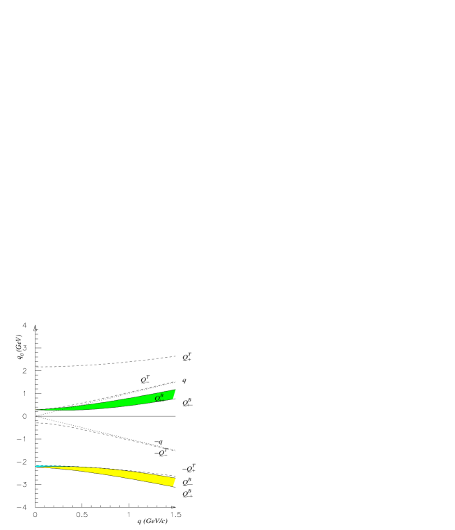
Figure 1: The singularities $Q^{B}$ and $Q^{T}$ of the function $U^{*[0]}_{rel}$ in the $({|{\bf q}|},q_{0})$ plane. Here, having in mind nucleons and $\Delta$’s, we have $m=0.938$ GeV and $M=1.232$ GeV. Solid lines denote the four singularities $Q^{B}_{\pm\pm}$ and dashed lines the $\pm Q^{T}_{\pm}$. Dotted lines denote the light cone. $k_{F}=0.264$ GeV/c. Light grey (yellow if in colors) region: $Q^{B}_{--}>q_{0}>Q^{B}_{-+}$; medium grey (cyan) region: $-Q^{T}_{-}>q_{0}>Q^{B}_{--}$; dark grey (green) region: $Q^{B}_{++}>q_{0}>Q^{B}_{+-}$; very dark (red) region (not visible in this figure): $Q^{T}_{-}>q_{0}>Q^{B}_{++}$.

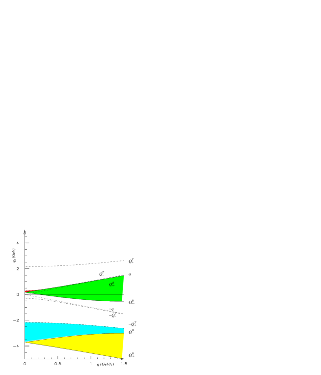
Figure 2: As fig. 1 but with $k_{F}=1.5$ GeV/c, in order to emphasize the region $Q^{T}_{-}>q_{0}>Q^{B}_{++}$, otherwise invisible.

6 The limiting cases

Having determined the response regions and the integers $k_{2}$ and $k_{3}$ we are now able to derive the response functions in the most general case. In this section we consider some specific limiting cases.

6.1 The case $M=m$

Here

$$Q^{T}_{-} = {|{\bf q}|}~{},$$ (82)

$$Q^{T}_{+} = \sqrt{4m^{2}+{|{\bf q}|}^{2}}$$ (83)

and the critical points $q_{\rm cr}^{(1)}$ and $q_{\rm cr}^{(2)}$ occur at $2k_{F}$ and $0$ respectively. Furthermore, $k_{F}^{\rm cr}=0$ and thus $Q^{B}_{+-}(k_{F})=E_{k_{F}-q}-E_{F}$ is always negative between $q_{\rm cr}^{3}=0$ and $q_{\rm cr}^{4}=2k_{F}$. Finally the $Q^{B}_{+\pm}(k_{F})$ always live in the space-like region.

The expressions for $U^{*}_{rel}$ given in Sec. 4 are still valid, provided we set $M=m$, which implies $\Delta\equiv\Delta^{*}=\sqrt{\frac{q^{2}-4m^{2}}{q^{2}}}$ and $\rho=1$. Concerning the imaginary parts, nothing changes in the particle-antiparticle domain, while in the particle-hole region, since $q_{\rm cr}^{2}$ vanishes, the response is confined to the range

$$Q^{B}_{+-}(k_{F})<q_{0}<Q^{B}_{++}(k_{F})$$

and $k_{2}$ and $k_{3}$ are given by (81).

6.2 The case $m=0$

This case may correspond to the excitation of a light quark to an $s$ or $c$ quark in a Quark Gluon Plasma.

Here

$$Q^{T}_{\pm}\equiv E^{*}_{q}~{},$$ (84)

while $q_{\rm cr}^{(1)}$ and $q_{\rm cr}^{(2)}$ tend to infinity: accordingly $Q^{T}_{\pm}$ and $Q^{B}_{+-}$ never coincide. Furthermore $k_{F}^{\rm cr}=M$. Finally it is immediately seen that $q_{\rm cr}^{(6)}\to\infty$, implying $Q^{B}_{++}>{|{\bf q}|}~{}\forall k_{F},~{}M$, while $q_{\rm cr}^{(5)}=M^{2}/(4k_{F})$. Thus the response region is represented by the intervals

$$Q^{B}_{+-}(k_{F}) <q_{0}< Q^{B}_{++}(k_{F})$$

$$Q^{B}_{-+}(k_{F}) <q_{0}< Q^{B}_{--}(k_{F})~{},$$

where Eq. (81) holds, and by

$$Q^{B}_{++}(k_{F}) <q_{0}< Q^{T}_{-}$$

$$Q^{B}_{--}(k_{F}) <q_{0}< -Q^{T}_{+}~{},$$

where instead (80) is valid.

Concerning the LF, since now $\rho=\Delta^{*}=1-\frac{M^{2}}{q^{2}}$ and $y^{*}_{\pm}=\frac{1}{2}\left(1-\frac{M^{2}}{q^{2}}\right)({|{\bf q}|}\pm q_{0})$, we end up with the expression

$$\begin{split}U^{*[0]}_{rel}\bigm{|}_{m=0}&=\frac{(2k_{F}+q_{0})q^{2}-M^{2}q_{0}}{32\pi^{2}{|{\bf q}|}q^{2}}\left\{\log\left|\frac{M^{2}-2k_{F}(q_{0}+{|{\bf q}|})-q^{2}}{M^{2}-2k_{F}(q_{0}-{|{\bf q}|})-q^{2}}\right|+i\pi k_{2}\right\}\\ &-\frac{q^{2}-M^{2}}{32\pi^{2}q^{2}}\left\{\log\left|\frac{(M^{2}-2k_{F}q_{0}-q^{2})^{2}-4k_{F}^{2}{|{\bf q}|}^{2}}{(M^{2}-q^{2})^{2}}\right|+i\pi k_{3}\right\}~{}.\end{split}$$ (85)

6.3 The case $M=m=0$.

Finally we consider the extreme situation where both masses vanish. Here the values $Q^{T}_{\pm}$ coincide with the light cone, while $Q^{B}_{\pm\pm}=\pm|k_{F}\pm{|{\bf q}|}|-k_{F}$ and inside the response region only the case of Eq. (81) occurs.

The expression of $U^{*}_{rel}$ further simplifies to

$$\begin{split}U^{*[0]}_{rel}\bigm{|}_{m=0}&=\frac{2k_{F}+q_{0}}{32\pi^{2}{|{\bf q}|}}\left\{\log\left|\frac{q^{2}+k_{F}(q_{0}+{|{\bf q}|})}{q^{2}+2k_{F}(q_{0}-{|{\bf q}|})}\right|+i\pi k_{2}\right\}\\ &-\frac{1}{32\pi^{2}}\left\{\log\left|\frac{{|{\bf q}|}^{2}-(2k_{F}+q_{0})^{2}}{q^{2}}\right|+i\pi k_{3}\right\}~{}.\end{split}$$ (86)

7 The spin 1/2 resonances

In this Section we explore the LFs associated to the excitations of the nucleon, addressing first the simpler case of the spin 1/2 resonances (e.g. the Roper ($N^{*}1440$) resonance). For sake of simplicity we disregard isospin, which simply yields a numerical factor.

7.1 The 0-index functions

Here the vertices we consider, beyond the identity, carry some $\gamma$-matrix structure of the type $\not\hskip-3.0ptp$ or $\not\hskip-3.0ptq$ times, eventually, a $\gamma_{5}$. Owing to the mass shell condition for the nucleon, $\not\hskip-3.0ptp=(\not\hskip-3.0ptp-m)+m$ can be replaced by $m$, since $\not\hskip-3.0ptp-m$ cancels with the nucleon propagator, leaving a $k_{F}$-independent term subtracted out by the renormalisation. The nucleon-hole case requires a separate discussion.

Similarly, $\not\hskip-3.0ptq=(\not\hskip-3.0ptp+\not\hskip-3.0ptq-M)-(\not\hskip-3.0ptp-m)-(M-m)$ leaves us with the identity times $M-m$ plus, however, a contact term, an occurrence reflecting our ignorance about the off-shell reaction mechanisms. Actually the $\not\hskip-3.0ptq$ vertex is redundant as far as the imaginary part of the LFs, and hence the response functions, are concerned. The real parts instead are altered by an extra contact term that matters in the response when higher orders (say, a RPA series) are accounted for.

In attempting to account for the different off-shell behaviour one meets a proliferation of complicated and mostly irrelevant terms. Thus here we confine ourselves to consider only the vertices ${\cal O}=I$ ($\sigma$-meson absorption), $\gamma_{5}$ and $\not\hskip-3.0ptq\gamma_{5}$ (pion absorption within the pseudoscalar and the pseudovector coupling). This last, at variance of the pseudoscalar coupling, correctly describes the $\pi^{0}$ suppression in the photo-production process and respects the chiral limit, owing to a further contact term added to the pseudoscalar vertex. Notice that the vertices containing a $\gamma_{5}$ are derived from the corresponding parity-conserving ones (up to, eventually, a sign) by replacing $m$ with $-m$.

For the 0-index LFs Eq. (27) applies and we only need to specify $A^{S}$ and $\lambda^{S}_{mn}$ in the various cases.

Considering first a scalar probe, the function $f_{ss}$ reads

$$\begin{split}f_{ss}(p,q)&={\rm Tr}(\not\hskip-3.0ptp+\not\hskip-3.0ptq+M)(\not\hskip-3.0ptp+m)=4(p^{2}+p\cdot q+Mm)\\ &=2\mathfrak{D}^{*}(p+q)-2\mathfrak{D}(p)+2Q_{+}~{},\end{split}$$ (87)

where use has been made of the identity (23) in the second line. Thus we get $A^{S}(q^{2})=2Q_{+}$ and $\lambda^{S}_{10}=2$. The term $2\mathfrak{D}(p)$ is cancelled by the renormalisation when studying the resonance-hole case, but it survives in the nucleon-hole one. In conclusion

$$\Pi^{*(0)}_{ss}(M;{|{\bf q}|},q_{0})=2T_{S+}^{*[1,0]}+2Q_{+}\Upsilon^{*[0]}_{+}(M;{|{\bf q}|},q_{0})~{}.$$ (88)

The other vertices are decoupled from the identity by parity conservation. For the pseudoscalar coupling ($\gamma_{5}$) we find

$$\Pi^{*(0)}_{psps}(M;{|{\bf q}|},q_{0})=-\Pi^{*(0)}_{ss}(M;{|{\bf q}|},q_{0})\biggm{|}_{m\to-m}~{}.$$ (89)

For the pseudovector coupling, introducing the notations

$$M_{T}=M+m\qquad\qquad\qquad\delta m=M-m~{},$$ (90)

we find $A^{S}=2M_{T}^{2}Q_{-}$ and $\lambda^{S}_{10}=2(\delta mM_{T}-q^{2}\rho)$, $\lambda^{S}_{20}=2$. As already outlined, in going from the pseudoscalar to the pseudovector LF the coefficient $A^{S}$ is multiplied by the expected factor $M_{T}^{2}$, but the contact term does not.

The pseudovector coupling conserves the axial current (or alternatively the existence of the Goldstone boson). Covariance would entail $\Pi^{*}_{PV}\sim q^{2}$, but, since it is broken, the Goldstone theorem only requires

$$\lim_{\begin{subarray}{c}q_{0}\to 0\\ {|{\bf q}|}\to 0\end{subarray}}\Pi^{*}_{PV}(M;{|{\bf q}|},q_{0})=0~{}.$$ (91)

Now we observe that

$$\Upsilon_{+}^{[0]}(M;0,0)=2U_{+}^{[0]}(M;0,0)=2\int\frac{d^{3}p}{(2\pi)^{3}}\frac{1}{2E_{p}}\frac{\theta(k_{F}-{|{\bf p}|})}{m^{2}-M^{2}}=-\frac{2}{M^{2}-m^{2}}\mathfrak{T}^{[0]}$$ (92)

and it is easily verified that the contact terms are tailored in such a way to exactly cancel $A^{S}\Upsilon_{+}^{[0]}$ in the limit $q\to 0$.

Finally the mixed pseudoscalar-pseudovector LF also exists: it has $A^{S}=2M_{T}Q_{-}$ and $\lambda^{S}_{10}=2\delta m$ while the pseudovector-pseudoscalar function has the opposite sign.

The nucleon-hole case must be considered aside because of the different structure of the contact terms. For example, the scalar-scalar response, owing to (87) leads to the manifestly vanishing contact term

$$-2i\int\frac{d^{4}p}{(2\pi)^{4}}\mathfrak{S}_{m}(p)+2i\int\frac{d^{4}p}{(2\pi)^{4}}\mathfrak{S}_{m}(p+q)~{}.$$

It is found that the only existing contact term pertains to the pseudovector-pseudovector case and is given by $4q^{2}\mathfrak{T}^{[0]}$.

7.2 The scalar-vector interference

In infinite nuclear matter a scalar probe can be transformed, through a resonance (nucleon)-hole propagator, into a vector one. Thus we shall consider, as before, the scalar-type vertices $I$ and $\gamma_{5}$. Concerning the vector-like vertices, 24 independent currents exist, 12 of them parity conserving and 12 parity-violating (see, e.g., Ref. [15]). However, currents embodying a $q^{\mu}$ (that can be extracted out of the integral) times a (pseudo-)scalar structure reduce to a 0-index LF, already handled in Sec. 7.1, times $q^{\mu}$. Further, neglecting contact terms, $\not\hskip-3.0ptp$ and $\not\hskip-3.0ptq$ are redundant and the Gordon identity

$$p^{\mu}=-\frac{1}{2}q^{\mu}+\frac{1}{4}(\not p+\not q-M)\gamma^{\mu}+\frac{1}{4}\gamma^{\mu}(\not p-m)\\ +\frac{1}{4}(M+m)\gamma^{\mu}-\frac{i}{4}\sigma^{\mu\nu}q_{\nu}$$ (93)

allows us to express the current $p^{\mu}$ in terms of the usual currents $\gamma^{\mu}$ and $\sigma^{\mu\nu}q_{\nu}$ only on the mass shell, while the off-mass-shell extension of the currents remains unpredictable.

Disregarding the huge variety of contact terms and $q^{\mu}$, only four independent currents survive, and they may be forced to be conserved by adding some suitable terms proportional to $q^{\mu}$. They read

$$j_{1}^{\mu}&=\gamma^{\mu}-\frac{\not\hskip-3.0ptqq^{\mu}}{q^{2}}\\ j_{2}^{\mu}=\frac{i}{2m}q_{\nu}\sigma^{\mu\nu}\\ j_{3,4}^{\mu}=j_{1,2}^{\mu}\gamma_{5}~{}.$$ (94)

Furthermore $j_{4}^{\mu}$ is expressible in terms of the other three currents by exploiting the charge conjugation symmetry.

Since all these current are conserved, only the first term of Eq. (36) is required. The functions $A^{V}_{xy}(q^{2})$ are listed, with a self-explanatory notation, in Table 1.

	$I\to j_{1}^{\mu}$	$I\to j_{2}^{\mu}$	$\gamma_{5}\to j_{3}^{\mu}$	$\gamma_{5}\to j_{4}^{\mu}$
$A^{(1)}_{xy}(q^{2})$	$4M_{T}$	$\dfrac{2}{m}q^{2}$	$4\delta m$	$-\dfrac{2}{m}q^{2}$

Table 1: The function $A^{V}_{xy}(q^{2})$ for the scalar-vector Lindhard function

7.3 The 2-indices response

	$j_{1}^{\mu}$	$j_{2}^{\mu}$
$j_{1}^{\nu}$	$-\dfrac{2Q_{-}}{q^{2}}$	$\dfrac{M_{T}}{mq^{2}}Q_{-}$
$j_{2}^{\nu}$	$-\dfrac{M_{T}}{mq^{2}}Q_{-}$	$\dfrac{M_{T}^{2}}{2m^{2}q^{2}}Q_{-}$

Table 2: The functions $A^{S}(q^{2})$ for the vector-vector parity conserving currents

	$j_{1}^{\mu}$	$j_{2}^{\mu}$
$j_{1}^{\nu}$	$8$	0
$j_{2}^{\nu}$	0	$2\dfrac{q^{2}}{m^{2}}$

Table 3: The functions $A^{LT}(q^{2})$ for the vector-vector parity conserving currents

We consider now the vector-vector response and distinguish between three different sets of LFs.

1. First we examine the parity conserving-parity conserving LFs (set up by the conserved currents $j_{1}^{\mu}$ and $j_{2}^{\mu}$), which are symmetric tensors. Thus only the functions $\Pi^{*L}$ and $\Pi^{*T}$ are required, that in turn need the knowledge of $A^{S}$, $A^{LT}$ and of the corresponding $\lambda$’s, according to (45) and (46). The $A^{S}$ are summarised in Table 3 and the $A^{LT}$ in 3. The contact terms $\lambda^{S}_{10}$ pertaining to $\Pi^{*S}$ are displayed in Table 5. The other contributions, namely the $\lambda^{LT}_{i0}(q^{2})$ are all vanishing. Instead a coefficient $\lambda^{S}_{20}$ survives for the $j_{2}^{\mu}j_{2}^{\nu}$ case and the relation $\lambda^{S}_{20}(j_{2}^{\mu}j_{2}^{\nu})=1/(2m^{2}q^{2})$ holds.

   	$j_{1}^{\mu}$	$j_{2}^{\mu}$
   $j_{1}^{\nu}$	$-\dfrac{2}{q^{2}}$	$\dfrac{\delta m}{mq^{2}}$
   $j_{2}^{\nu}$	$-\dfrac{\delta m}{mq^{2}}$	$-\dfrac{q^{2}\rho-M_{T}\delta m}{2m^{2}q^{2}}$

   Table 4: The contact terms $\lambda^{S}_{10}(q^{2})$ for the vector-vector parity conserving currents

   	$j_{1}^{\mu}$	$j_{2}^{\mu}$
   $j_{3}^{\nu}$	$4i$	$-2i\dfrac{M_{T}}{m}$
   $j_{4}^{\nu}$	$-2i\dfrac{\delta m}{m}$	$i\dfrac{M_{T}\delta m}{m^{2}}$

   Table 5: The functions $A^{*V}(q^{2})$ for the vector-vector parity conserving-parity violating currents

2. Next we consider parity conserving-parity violating LFs (currents $j_{1}^{\mu}$ and $j_{2}^{\mu}$ at the incoming vertex, $j_{3}^{\mu}$ and $j_{4}^{\mu}$ at the outgoing one). Here the tensors are antisymmetric and Eq. (49) applies with the second term only, namely

   $$q_{\lambda}\mathfrak{N}^{\sigma}g_{\sigma\rho}\epsilon^{\mu\nu\rho\lambda}\Pi^{*V}_{xy-}(M;{|{\bf q}|},q_{0})~{},$$

   with $\Pi^{*V}_{xy-}$ defined by Eq. (34). The required functions $A^{*V}(q^{2})$ are displayed in Table 5. No contact term exists. The case $j_{2}^{\mu}j_{4}^{\nu}$ would provide a non-vanishing function $\lambda^{V}_{10}$, but actually $T^{[1,0]}_{x-}=0$. Finally if we reverse the vertices the following relation holds:

   $$\Pi^{(2)\mu\nu}_{j_{n}^{\mu}j_{m}^{\nu}}=(-1)^{m+1}\Pi^{(2)\mu\nu}_{j_{m}^{\mu}j_{n}^{\nu}}~{},~{}~{}~{}~{}~{}m=1,2~{},~{}~{}~{}~{}~{}n=3,4~{}.$$ (95)

3. The parity violating-parity violating LFs are derived from the parity conserving-parity conserving ones through the simple relations

   $$\Pi^{*}_{j_{3},j_{3,4}}&=\Pi^{*}_{j_{1},j_{1,2}}|_{m\to-m}~{},\\ \Pi^{*}_{j_{4},j_{3,4}}=-\Pi^{*}_{j_{2},j_{1,2}}|_{m\to-m}~{}.$$ (96)

Again the nucleon-hole case differs from the above only for the contact terms, because a direct evaluation shows that the various $\mathfrak{Q}$ are just the limits of the $\mathfrak{Q}^{*}$ for $M\to m$. Only one contact term exists for the case $j_{1}^{\mu}j_{1}^{\nu}$, with $\lambda_{10}^{S}=-2/q^{2}$.

8 The spin 3/2 resonances

We consider now the excitation of a nucleon to a spin 3/2 resonance (specifically the $\Delta(1232)$ ), assumed to be stable. The resonance is described by a vector-spinor field $\psi_{\mu}$ obeying the Rarita-Schwinger equations

$$(i\not\hskip-3.0pt\partial-m)\psi_{\mu}&=0\\ \gamma^{\mu}\psi_{\mu}=0\\ \partial^{\mu}\psi_{\mu}=0$$ (97)

(the last line is, more properly, a constraint) which can be deduced from the Lagrangian [16]

$${\cal L}=\bar{\psi}_{\mu}\Bigl{\{}(i\not\hskip-3.0pt\partial-M)g^{\mu\nu}+i\omega(\gamma^{\mu}\partial^{\nu}+\partial^{\mu}\gamma^{\nu})\\ +\frac{i}{2}\left(3\omega^{2}+2\omega+1\right)\gamma^{\mu}\not\hskip-3.0pt\partial\gamma^{\nu}+\left(3\omega^{2}+3\omega+1\right)M\gamma^{\mu}\gamma^{\nu}\Bigr{\}}\psi_{\nu}~{},$$ (98)

$\omega$ ($\not=-1/2$) being a free parameter. Each value of $\omega$ leads to the equations of motion (97), but does not prevent the occurrence of a spin 1/2 component in the $\omega$-dependent vector-spinor $\psi_{\mu}$. Thus, to rule out these unwanted components, one usually introduces the projection operator on the spin 3/2 space, which reads (in momentum space)

$$P_{3/2}^{\mu\nu}=g^{\mu\nu}-\frac{1}{3}\gamma^{\mu}\gamma^{\nu}-\frac{1}{3p^{2}}\left(\not\hskip-3.0ptp\gamma^{\mu}p^{\nu}+p^{\mu}\gamma^{\nu}\not\hskip-3.0ptp\right)~{},$$ (99)

or, sometimes, its on-shell reduction

$$P_{3/2}^{\mu\nu}\rightarrow P_{3/2}^{\mu\nu}\bigm{|}_{p^{2}\to M^{2}}~{}.$$ (100)

The most common choices are $\omega=-1/3$, that leads to the Rarita-Schwinger result, and $\omega=-1$, that corresponds to the Lagrangian

$${\cal L}=\bar{\psi}_{\mu}\left\{-\epsilon^{\mu\nu\lambda\rho}\gamma^{5}\gamma_{\lambda}\partial_{\rho}-iM\sigma^{\mu\nu}\right\}\psi_{\nu}~{}.$$ (101)

Another Lagrangian has been recently proposed, namely [17]

$${\cal L}=\bar{\psi}_{\mu}\left\{-\epsilon^{\mu\nu\lambda\rho}\gamma^{5}\gamma_{\lambda}\partial_{\rho}-Mg^{\mu\nu}\right\}\psi_{\nu}$$ (102)

in order to solve the so-called Velo-Zwanziger disease [18, 19]. However we do not discuss such a Lagrangian here, as it describes a resonance propagating in an external electro-magnetic field with the (minimally coupled) $\Delta\Delta\gamma$ vertex, while we only consider non-minimal $N$-$\Delta$ transitions. Furthermore, the proposal (102) is seriously plagued by the occurrence of a pole at $p^{2}=M^{2}/4$, as the evaluation of the propagator (the inverse of $\Gamma^{\mu\nu}$) shows.

Sticking to the more sound form (98), observe that different values of $\omega$ not only alter the mixing between 3/2 and 1/2 spin, but also affect the off-shell behaviour of the $\Delta$-hole propagator, that in fact reads

$$\Delta^{\mu\nu}=\frac{\not\hskip-3.0ptp+M}{p^{2}-M^{2}}\left\{g^{\mu\nu}-\frac{1}{3}\gamma^{\mu}\gamma^{\nu}-\frac{1}{3M}(\gamma^{\mu}p^{\nu}-\gamma^{\nu}p^{\mu})-\frac{2}{3M^{2}}p^{\mu}p^{\nu}\right\}\\ +\frac{1+\omega}{6M^{2}(1+2\omega)^{2}}\Bigl{\{}(1+3\omega)(\gamma^{\mu}p^{\nu}+\gamma^{\nu}p^{\mu})+(1+\omega)(\gamma^{\mu}p^{\nu}-\gamma^{\nu}p^{\mu})\\ -2M\omega\gamma^{\mu}\gamma^{\nu}+(1+\omega)\not\hskip-3.0ptp\gamma^{\mu}\gamma^{\nu}\Bigr{\}}$$ (103)

Remarkably the choice $\omega=-1$ cancels in (103) all the terms with no analytic structure, which would otherwise contribute to the contact terms in the $\Delta$-hole LF.

8.1 The 0-index $\Delta$-hole Lindhard functions

Here the vertices have the form $\bar{\psi}j^{\mu}\psi_{\mu}$ or $\bar{\psi}j^{\mu}P_{3/2}^{\mu\nu}\psi_{\nu}$, where $j^{\mu}$ could be taken from Eq. (94) plus the non-conserved $q^{\mu}$ and $\gamma_{5}q^{\mu}$. Clearly

$$f_{xy}(p,q)={\rm Tr}(\not\hskip-3.0ptp+m){j_{x}}_{\mu}\Delta^{\mu\nu}{j_{y}}_{\nu}$$ (104)

or, alternatively,

$$f_{xy}(p,q)={\rm Tr}(\not\hskip-3.0ptp+m){j_{x}}_{\mu}P_{3/2}^{\mu\lambda}\Delta^{\lambda}_{\ \rho}P_{3/2}^{\rho\nu}{j_{y}}_{\nu}~{}.$$ (105)

However, the vector $\gamma^{\mu}$ is constrained by (97b) so that this current, when contracted with $\Delta^{\mu\nu}$, is vanishing on shell, does not develop an imaginary part and consequently it can only contribute to the contact terms. The same occurs for $\gamma^{\mu}\gamma_{5}$. Furthermore $\sigma^{\mu\lambda}q_{\lambda}$ can be replaced by $q^{\mu}$ because

$$\sigma^{\mu\nu}q_{\nu}\psi_{\mu}=iq^{\mu}\psi_{\mu}~{}.$$

Thus only the two currents

$$j_{1}(N\Delta)^{\mu}&=q^{\mu}\\ j_{2}(N\Delta)^{\mu}=q^{\mu}\gamma_{5}$$ (106)

actually matter, at least for the part carrying analytic structure. Since we are dealing with a 0-index LF, the structure is given by (27). With self-explanatory notations the non-vanishing $A^{S}$ are found to be

$$A^{S}_{j_{1}^{\mu}j_{1}^{\nu}}=-\frac{Q_{-}Q_{+}^{2}}{3M^{2}}~{},~{}~{}~{}~{}~{}A^{S}_{j_{2}^{\mu}j_{2}^{\nu}}=\frac{Q_{-}^{2}Q_{+}}{3M^{2}}~{}.$$ (107)

Concerning the contact terms, we will not give a detailed list for all the 24 currents, because they all explicitly depend upon $\omega$ and display a double pole at $\omega=-1/2$: hence they can diverge and the real part of the LFs becomes unpredictable. As a consequence, the RPA series based on the $\Delta$-hole excitation (and, similarly, any calculation beyond the bare Free Fermi Gas) becomes unreliable.

The same happens if we use the expression (105) taking however the projection operator in the form (100). We get indeed Eqs. (107) for the functions $A^{S}$, but again the contact terms display a double pole in $\omega$.

Finally we can take the projection operator in the form (99). Now the expressions (107) are again valid, but the contact terms are independent of $\omega$ and, furthermore, they do not change in replacing $q^{\mu}$ with $i\sigma^{\mu\nu}q_{\nu}$. They display however a factor $(p+q)^{-2}$ coming from the projection operator Eq. (99). For instance, in the current $j_{1}{(N\Delta)}^{\mu}$ they take the form

$$\int\frac{d^{3}p}{(2\pi)^{3}}\frac{1}{2E_{p}}\Biggl{\{}\frac{(m^{2}-q^{2})^{2}(m^{2}+2mM-q^{2})}{3M^{2}(p+q)^{2}}\Bigm{|}_{p^{2}=m^{2}}\\ +\frac{1}{3}(2q^{2}-2p\cdot q-M^{2}-2mM)\Biggr{\}}\theta(k_{F}-{|{\bf p}|})+(q_{0}\longleftrightarrow-q_{0})~{}.$$

Here the first term is just the function $U^{*[0]}_{\rm rel}$ evaluated at $M=0$, thus explaining the introduction of the factor $B_{xy}^{S}(q^{2})\Upsilon^{*[0]}_{\pm}(M=0;{|{\bf q}|},q_{0})$ in Eq. (27). Explicitly the case $(j_{1}^{\mu}j_{1}^{\nu})$ requires

$$B^{S}_{j_{1}^{\mu}j_{1}^{\nu}}=\frac{(m^{2}-q^{2})^{2}(m^{2}+2mM-q^{2})}{3M^{2}}$$ (108)

and furthermore $\lambda^{S}_{10}=(m^{2}-2mM-2M^{2}+3q^{2})/3$ and $\lambda^{S}_{20}=-1/3$. Finally,

$$\Pi^{*(0)}_{j_{2}^{\mu}j_{2}^{\nu}}=-\Pi^{*(0)}_{j_{1}^{\mu}j_{1}^{\nu}}\bigm{|}_{m\to-m}~{}.$$ (109)

8.2 The 1-index function

Now we consider the case of the transition from a scalar to a vector term, which leads to a 1-index LF. Here, besides the vectors discussed in the previous subsection, we also need a tensor operator yielding a vector when contracted with the $\Delta$ propagator. Again one can set up a vast amount of tensors: we limit ourselves to those which give LFs with the same analytic structure, ignoring extra contact terms.

We are thus left with eight possible currents, namely

$$j^{\nu}_{X}=\overline{\psi}\Gamma^{\mu\nu}_{X}\psi_{\mu}+{\rm h.~{}c.}$$ (110)

with

$$\Gamma^{\mu\nu}_{M(V)}&=-\frac{3}{2}\frac{\mu+1}{Q_{+}}\epsilon^{\mu\nu\alpha\beta}p_{\alpha}q_{\beta}\\ \Gamma^{\mu\nu}_{E(V)}=-\Gamma^{\mu\nu}_{M(V)}-i\frac{3}{2}\frac{\mu+1}{Q_{+}Q_{-}}4\epsilon^{\mu\sigma\alpha\beta}p_{\alpha}q_{\beta}\epsilon^{\nu}_{\;\sigma\gamma\delta}p^{\gamma}q^{\delta}\gamma_{5}\\ \Gamma^{\mu\nu}_{C(V)}=-i\frac{3}{2}\frac{\mu+1}{Q_{+}Q_{-}}2q^{\mu}\left(q^{2}p^{\nu}-p\cdot qq^{\nu}\right)\gamma_{5}\\ \Gamma^{\mu\nu}_{M(A)}=-i\frac{3}{2}\frac{\mu-1}{Q_{-}}\left[-2\gamma_{5}\epsilon^{\mu\nu\alpha\beta}p_{\alpha}q_{\beta}-\frac{2}{Q_{+}}\epsilon^{\mu\sigma\alpha\beta}p_{\alpha}q_{\beta}\epsilon^{\nu}_{\;\sigma\gamma\delta}p^{\gamma}q^{\delta}\right]\\ \Gamma^{\mu\nu}_{E(A)}=-i\frac{3}{2}\frac{\mu-1}{Q_{+}Q_{-}}2\epsilon^{\mu\sigma\alpha\beta}p_{\alpha}q_{\beta}\epsilon^{\nu}_{\;\sigma\gamma\delta}p^{\gamma}q^{\delta}\\ \Gamma^{\mu\nu}_{C(A)}=i\frac{3}{2}\frac{\mu-1}{Q_{+}Q_{-}}2q^{\mu}\left(q^{2}p^{\nu}-p\cdot qq^{\nu}\right)\\ \Gamma^{\mu\nu}_{S(V)}=g^{\mu\nu}\gamma_{5}\\ \Gamma^{\mu\nu}_{S(A)}=g^{\mu\nu}$$ (111)

(here $\mu=M/m$). We have followed in the above the work of Devenish et al. [20]: these author show that, for a transition from a nucleon to a higher spin resonance (not necessarily 3/2), only three conserved currents enter the parity-conserving sector and as many the parity-violating one. In the low momentum regime tensors associated to these six currents correspond to the multipoles M1, E2, C2, M2, E1, C1 (the first three parity conserving, the other parity violating). We have added two other currents, which are not conserved, thus exhausting all the possibilities.

We see that again LFs with only one vector index exists, but they only occur between a Coulomb multipole and the non-conserved currents (106). The case $(j_{2}^{\mu}\Gamma_{C(V)})$ contains only a $t^{\mu}$ in the integrand, thus the expression (34) applies (first term in (36)) with

$$A^{V}_{j_{2}^{\mu}\Gamma_{C(V)}}&=-i\frac{M_{T}}{mM^{2}}Q_{-}\\ B^{V}_{j_{2}^{\mu}\Gamma_{C(V)}}=i\frac{M_{T}}{mM^{2}}\frac{(m^{2}-q^{2})^{2}(m^{2}-2mM-q^{2})q^{2}}{Q_{+}Q_{-}}\\ \lambda^{V}_{10}=\frac{iM_{T}q^{2}}{m}\frac{m^{2}+2mM-2M^{2}+3q^{2}}{Q_{+}Q_{-}}\\ \lambda^{V}_{20}=-\frac{iM_{T}q^{2}}{mQ_{+}Q_{-}}~{}.$$ (112)

The case $(j_{2}^{\mu}\Gamma_{S(V)})$ requires the full expression (36) and we find (since $T^{[1,0]}_{S-}=0$)

$$A^{V}_{j_{2}^{\mu}\Gamma_{S(V)}}&=\frac{2Q_{-}}{3M^{2}}(q^{2}+M^{2}-m^{2})\\ B^{V}_{j_{2}^{\mu}\Gamma_{S(V)}}=\frac{2}{3M^{2}}(m^{2}-2mM-q^{2})(m^{2}-q^{2})\\ \lambda^{V}_{10}=\frac{2}{3}\\ A^{S}_{j_{2}^{\mu}\Gamma_{S(V)}}=\frac{Q_{-}^{2}Q_{+}q^{2}}{3M^{2}}\\ B^{S}_{j_{2}^{\mu}\Gamma_{S(V)}}=-\frac{1}{3M^{2}q^{2}}(m^{2}-2mM-q^{2})(m^{2}-q^{2})^{2}\\ \lambda^{S}_{20}=\frac{1}{3q^{2}}~{}.$$ (113)

The LFs with opposite parity simply obtain as

$$\Pi^{*(1)\mu}_{j_{1},\Gamma_{x(A)}}({|{\bf q}|},q_{0})=-\Pi^{*(1)\mu}_{j_{2},\Gamma_{x(V)}}({|{\bf q}|},q_{0})\bigm{|}_{m\to-m}~{}.$$ (114)

8.3 The 2-indices functions

8.3.1 Parity conserving-parity conserving Lindhard functions

We consider first of all the couplings $M1$, $E2$ and $C2$ (parity conserving) in both vertices. These currents being conserved, we can directly apply Eqs. (45) and (46). Hence the functions $A_{xy}^{S}$, $A_{xy}^{LT}$ and the corresponding $\lambda$’s are needed. Remarkably, $A_{xy}^{S}$ and $A_{xy}^{LT}$ are diagonal with respect to the channel indices and are quoted in Tables 7 and 7 respectively.

$\Gamma_{M(V)}$	$\Gamma_{E(V)}$	$\Gamma_{C(V)}$
$\dfrac{3M_{T}^{2}}{4m^{2}q^{2}}Q_{-}$	$\dfrac{9M_{T}^{2}}{4m^{2}q^{2}}Q_{-}$	$0$

Table 6: The $A^{S}(q^{2})$ functions for the vector-vector $\Delta$-$N$ parity conserving currents

$\Gamma_{M(V)}$	$\Gamma_{E(V)}$	$\Gamma_{C(V)}$
$\dfrac{3M^{2}_{T}q^{2}}{m^{2}Q_{+}}$	$\dfrac{9M_{T}^{2}q^{2}}{m^{2}Q_{+}}$	$-\dfrac{3M_{T}^{2}q^{4}}{m^{2}M^{2}Q_{+}}$

Table 7: The $A^{LT}(q^{2})$ functions for the vector-vector $\Delta$-$N$ parity conserving currents

Instead, a contact term coupling the multipoles $M1$ and $E2$ exists (it is reported in Appendix C together with all the other contact terms).

Both the multipoles $M1$ and $E2$ display the structure of Eqs. (45) and (46) with, however, $B^{x}=0$, while in the Coulomb multipole $C2$ the contribution proportional to $\Pi^{*S}$ is absent. $A^{LT}$ is given in Table 7 and furthermore

$$B^{LT}_{C(V)C(V)}(q^{2})=\frac{3M_{T}^{2}q^{4}}{m^{2}M^{2}Q_{+}^{2}Q_{-}^{2}}(m^{2}-q^{2})^{2}(m^{2}-2mM-q^{2})~{}.$$ (115)

Observe also that in this sector $\Pi^{*(2)\mu\nu}_{xy}=\Pi^{*(2)\mu\nu}_{yx}$.

8.3.2 Parity conserving-parity violating Lindhard functions

This kind of LF is antisymmetric in the indices $\mu$, $\nu$ and takes the form

$$q_{\lambda}\mathfrak{N}^{\sigma}g_{\sigma\rho}\epsilon^{\mu\nu\rho\lambda}\Pi^{*V}_{xy-}(M;{|{\bf q}|},q_{0})$$

(see Eq. (34)). We thus need to specify the functions $A^{V}_{xy}$ and the contact terms. The only non-vanishing $A^{V}_{xy}$ are

$$A^{V}_{E(V)M(A)}(q^{2})=3A^{V}_{M(V)E(A)}(q^{2})=-\frac{9iM_{T}\delta m}{2m^{2}}$$ (116)

and for the relevant contact terms (not $\lambda^{V}_{10}$ $T^{[1,0]}_{V-}=0$) we refer the reader to Appendix C. Moreover,

$$\Pi^{0\mu\nu}_{x(A)y(V)}=-\Pi^{0\mu\nu}_{x(V)y(A)}$$ (117)

(with $x,y=M,E,C$).

8.3.3 Parity violating-parity violating Lindhard functions

The functions $A^{S}$, $A^{LT}$ and $B^{LT}$ follow from the parity conserving-parity conserving case with the replacements

$$A^{x}_{E(A)E(A)}(q^{2})=-A^{x}_{M(V)M(V)}(q^{2})\bigm{|}_{m\to-m}~{},\\ A^{x}_{M(A)M(A)}(q^{2})=-A^{x}_{E(V)E(V)}(q^{2})\bigm{|}_{m\to-m}~{},\\ A^{LT}_{C(A)C(A)}=-A^{LT}_{C(V)C(V)}\bigm{|}_{m\to-m}~{},B^{LT}_{C(A)C(A)}=-B^{LT}_{C(V)C(V)}\bigm{|}_{m\to-m}~{}.$$ (118)

As for the parity conserving-parity conserving case the rule (involving contact terms) $\Pi^{*(2)\mu\nu}_{xy}=\Pi^{*(2)\mu\nu}_{yx}$ holds. The contact terms (see Appendix C) have a quite involved structure.

8.3.4 Lindhard functions involving non-conserved currents

A LF having the first vertex $M(V)$ or $E(V)$ and the second $S(V)$ (this last corresponds to a non-conserved current) is non-vanishing and has the structure of Eq. (40) (a symmetric LF obeying the current conservation law). Thus it can be expressed in terms of Eqs. (39) with

$$3A^{S}_{M(V)S(V)}=A^{S}_{E(V)S(V)}=\frac{3iM_{T}Q_{-}}{2mq^{2}}$$ (119)

and

$$3A^{LT}_{M(V)S(V)}=A^{LT}_{E(V)S(V)}=\frac{6iM_{T}q^{2}}{mQ_{+}}~{}.$$ (120)

The same happens for $\Pi^{*(2)\mu\nu}_{E(A)S(A)}$ with

$$A^{S}_{E(A)S(A)}=-i\frac{\delta mQ_{+}}{mq^{2}}~{},~{}~{}~{}~{}~{}~{}~{}A^{LT}_{E(A)S(A)}=-4i\frac{\delta mq^{2}}{mQ_{-}}~{},$$ (121)

while $\Pi^{*(2)\mu\nu}_{M(A)S(A)}$ only displays contact terms (see Appendix C).

The LF $\Pi^{*(2)\mu\nu}_{C(V)S(V)}$ has a different structure: it contains a symmetric current-conserving term, as in Eq. (40), with $A^{S}_{C(V)S(V)}=0$ and

$$A^{LT}_{C(V)S(V)}&=\frac{2iM_{T}q^{2}}{mM^{2}Q_{+}}\left[m^{2}-M^{2}-q^{2}\right]\\ B^{LT}_{C(V)S(V)}=-\frac{2iM_{T}q^{2}}{mM^{2}Q_{+}Q_{-}}(m^{2}-q^{2})(m^{2}-2mM-q^{2})$$ (122)

plus the following term proportional to $q^{\nu}$

$$\mathfrak{N}^{\mu}q^{\nu}\Bigl{[}-\frac{iM_{T}Q_{-}}{mM^{2}}\mathfrak{Q}^{*V}_{-}\\ +\frac{iM_{T}}{mM^{2}Q_{+}Q_{-}}(m^{2}-q^{2})^{2}(m^{2}-2mM-q^{2})\mathfrak{Q}^{*V}_{-}(M=0)\\ +\sum_{m}\lambda^{V}_{m0}T^{*[m-1,0]}_{V-}({|{\bf q}|},q_{0})\Bigr{]}~{},$$ (123)

with the contact terms given in Appendix C. The symmetry relation

$$\Pi^{*(2)\mu\nu}_{C(A)S(A)}=-\Pi^{*(2)\mu\nu}_{C(V)S(V)}\bigm{|}_{m\to-m}$$ (124)

holds.

The functions with initial vertex $M(A)$ and $E(A)$ and final vertex $S(V)$, as well as $\Pi^{*(2)\mu\nu}_{M(V)S(A)}$ and $\Pi^{*(2)\mu\nu}_{S(V)S(A)}$ are antisymmetric and are given by the second term of Eq. (49), namely

$$q_{\lambda}\mathfrak{N}^{\sigma}g_{\sigma\rho}\epsilon^{\mu\nu\rho\lambda}\Pi^{*V}_{xy-}(M;{|{\bf q}|},q_{0})~{},$$

with

$$A^{V}_{M(A)S(V)} =3A^{V}_{E(A)S(V)}=-3\frac{\delta m}{m}~{},$$ (125)

$$A^{V}_{M(V)S(A)} =\frac{2M_{T}}{m}$$ (126)

and

$$A^{V}_{S(V)S(A)} =\frac{4i}{3}~{},$$ (127)

while $\Pi^{*(2)\mu\nu}_{E(V)S(A)}$ has only contact terms and $\Pi^{*(2)\mu\nu}_{C(A)S(V)}=\Pi^{*(2)\mu\nu}_{C(V)S(A)}=0$.

Next we consider the symmetric function $\Pi^{*(2)\mu\nu}_{S(V)S(V)}$. Since the current is not conserved, it is contributed to by all the terms in Eq. (47). Thus it displays a conserved part, which has

$$A^{S}_{S(V)S(V)}&=-\frac{4Q_{-}}{3q^{2}}\\ A^{LT}_{S(V)S(V)}=\frac{4Q_{-}}{3M^{2}}\\ B^{LT}_{S(V)S(V)}=\frac{4(q^{2}-m^{2}+2mM)}{3M^{2}}$$ (128)

plus a non-conserved one (last two terms in (47)). The latter requires the knowledge of $\Pi^{*V}_{S(V)S(V)-}$ - in turn fixed by (see Eq. (34))

$$A^{V}_{S(V)S(V)} = \frac{2Q_{-}}{3M^{2}q^{2}}(M^{2}-m^{2}+q^{2})$$ (129)

$$B^{V}_{S(V)S(V)} = \frac{2(m^{2}-q^{2})(m^{2}-2mM-q^{2})}{3M^{2}q^{2}}~{}.$$ (130)

Finally for the third term, which, being proportional to $q^{\mu}q^{\nu}$, is associated to a scalar quantity, as in Eq. (27), we get

$$\tilde{A}^{S}_{S(V)S(V)} = \frac{Q_{-}^{2}Q_{+}}{3M^{2}q^{4}}$$ (131)

$$B^{S}_{S(V)S(V)} = -\frac{(m^{2}-q^{2})^{2}(m^{2}-2mM-q^{2})}{3M^{2}q^{4}}~{}.$$ (132)

Again the symmetry relation

$$\Pi^{*(2)\mu\nu}_{S(A)S(A)}=-\Pi^{*(2)\mu\nu}_{S(V)S(V)}\bigm{|}_{m\to-m}$$ (133)

holds.

Note that the interchange of the initial and final vertex entails an interchange also of the indices $\mu$ and $\nu$.

Appendix A The elementary functions $T^{*[m,n]}$

The functions defined in Eq. (26) are given by

$$T^{*[1,0]}_{S+} = 2\mathfrak{T}^{[0]}$$ (134)

$$T^{*[2,0]}_{S+} = 2q^{2}\rho\mathfrak{T}^{[0]}$$ (135)

$$T^{*[2,0]}_{S-} = 4q_{0}\mathfrak{T}^{[1]}$$ (136)

$$T^{*[3,0]}_{S+} = -\frac{2}{3}(4m^{2}{|{\bf q}|}^{2}-3\rho^{2}q^{4})\mathfrak{T}^{[0]}+\frac{8}{3}(3q_{0}^{2}+{|{\bf q}|}^{2})\mathfrak{T}^{[2]}$$ (137)

$$T^{*[4,0]}_{S+} = 2\rho q^{2}(\rho^{2}q^{4}-4m^{2}{|{\bf q}|}^{2})\mathfrak{T}^{[0]}+8\rho q^{2}(3q_{0}^{2}+{|{\bf q}|}^{2})\mathfrak{T}^{[2]}$$ (138)

$$T^{*[5,0]}_{S+} = 2\left[\left(q^{4}\rho^{2}-4m^{2}{|{\bf q}|}^{2}\right)^{2}-\frac{64}{5}m^{4}{|{\bf q}|}^{4}\right]\mathfrak{T}^{[0]}$$

$$+ \left[16q^{4}\rho^{2}(3q_{0}^{2}+{|{\bf q}|}^{2})-\frac{64}{5}m^{2}{|{\bf q}|}^{2}(5q_{0}^{2}+{|{\bf q}|}^{2})\right]\mathfrak{T}^{[2]}$$

$$+ 32\left[\left(q_{0}^{2}+{|{\bf q}|}^{2}\right)^{2}-\frac{4}{5}{|{\bf q}|}^{4}\right]\mathfrak{T}^{[4]}$$

$$T^{*[1,0]}_{V+} = -2\frac{{|{\bf q}|}^{2}}{q^{2}}\mathfrak{T}^{[1]}$$ (140)

$$T^{*[2,0]}_{V+} = -2\rho{|{\bf q}|}^{2}\mathfrak{T}^{[1]}$$ (141)

$$T^{*[2,0]}_{V-} = \frac{4q_{0}{|{\bf q}|}^{2}}{3q^{2}}\left(m^{2}\mathfrak{T}^{[0]}-4\mathfrak{T}^{[2]}\right)$$ (142)

$$T^{*[3,0]}_{V-} = 2\rho{|{\bf q}|}^{2}T^{*[2,0]}_{V-}$$ (143)

$$T^{*[4,0]}_{V-} = \frac{4m^{2}q_{0}{|{\bf q}|}^{2}}{q^{2}}\left(q^{4}\rho^{2}-\frac{4}{5}m^{2}{|{\bf q}|}^{2}\right)\mathfrak{T}^{[0]}$$

$$- \frac{16q_{0}{|{\bf q}|}^{2}}{q^{2}}\left[q^{4}\rho^{2}-m^{2}\left(q_{0}^{2}+\frac{7}{5}{|{\bf q}|}^{2}\right)\right]\mathfrak{T}^{[2]}$$

$$- \frac{32q_{0}{|{\bf q}|}^{2}}{q^{2}}\left[q_{0}^{2}+\frac{3}{5}{|{\bf q}|}^{2}\right]\mathfrak{T}{[4]}$$

$$T^{*[1,0]}_{L+} = -\frac{2{|{\bf q}|}^{2}}{3q^{4}}\left[m^{2}q_{0}^{2}\mathfrak{T}^{[0]}-(q^{2}+4{|{\bf q}|}^{2})\mathfrak{T}^{[2]}\right]$$ (145)

$$T^{*[2,0]}_{L+} = q^{2}\rho T^{*[1,0]}_{L+}$$ (146)

$$T^{*[3,0]}_{L+} = -\frac{2}{3}\frac{m^{2}q_{0}^{2}{|{\bf q}|}^{2}}{q^{4}}\left[q^{4}\rho^{2}-\frac{12}{5}m^{2}{|{\bf q}|}^{2}\right]\mathfrak{T}^{[0]}$$

$$+ \frac{2}{3}\frac{{|{\bf q}|}^{2}}{q^{4}}\left[(q_{0}^{2}+3{|{\bf q}|}^{2})q^{4}\rho^{2}-\frac{4}{5}m^{2}(q_{0}^{2}+5{|{\bf q}|}^{2})({|{\bf q}|}^{2}+5q_{0}^{2})\right]\mathfrak{T}^{[2]}$$

$$+ \frac{8}{3}\frac{{|{\bf q}|}^{2}}{q^{4}}\left[q^{4}+\frac{48}{5}q_{0}^{2}q^{2}\right]\mathfrak{T}{[4]}$$

$$T^{*[1,0]}_{T+} = -\frac{4}{3}m^{2}\mathfrak{T}^{[0]}+\frac{4}{3}\mathfrak{T}^{[2]}$$ (148)

$$T^{*[2,0]}_{T+} = q^{2}\rho T^{*[1,0]}_{T+}$$ (149)

$$T^{*[3,0]}_{T+} = -\frac{4}{3}m^{2}\left[q^{4}\rho^{2}-\frac{4}{5}m^{2}{|{\bf q}|}^{2}\right]\mathfrak{T}^{[0]}$$

$$+ \frac{4}{3}\left[q^{4}\rho^{2}-4m^{2}\left(q_{0}^{2}+\frac{2}{5}{|{\bf q}|}^{2}\right)\right]\mathfrak{T}^{[2]}$$

$$+ \frac{16}{3}\left[q_{0}^{2}+\frac{1}{5}{|{\bf q}|}^{2}\right]\mathfrak{T}^{[4]}~{}.$$

Appendix B The elementary functions $U^{*[n]}$

In Sec. 4 we have derived the functions $U^{*[0]}_{rel}$. Actually we also need $U^{*[1]}_{rel}$ and $U^{*[2]}_{rel}$, which be be provided in this appendix. It is clear from the derivation of $U^{*[0]}_{rel}$ that the entire class of functions defined by Eq. (18) has a common structure, namely

$$U^{*[n]}_{rel}=\alpha_{0}^{[n]}+\alpha_{1}^{[n]}l_{1}+\alpha_{2}^{[n]}l_{2}+\alpha_{3}^{[n]}l_{3}~{}.$$ (152)

The coefficients are given by

$$\alpha_{0}^{[0]}&=0\\ \alpha_{1}^{[0]}=-\frac{\rho}{16\pi^{2}}\\ \alpha_{2}^{[0]}=\frac{q_{0}\rho+2E_{F}}{32\pi^{2}{|{\bf q}|}}\\ \alpha_{3}^{[0]}=-\frac{\Delta^{*}}{64\pi^{2}}\\ \alpha_{0}^{[1]}=-\dfrac{\rho k_{F}}{32\pi^{2}}\\ \alpha_{1}^{[1]}=\frac{q_{0}}{32\pi^{2}}\left[\rho^{2}-\frac{2m^{2}}{q^{2}}\right]\\ \alpha_{2}^{[1]}=\frac{1}{128\pi^{2}{|{\bf q}|}}\left[4k_{F}^{2}-({|{\bf q}|}^{2}+q_{0}^{2})\rho^{2}+\frac{4m^{2}q_{0}^{2}}{q^{2}}\right]\\ ~{}\\ \alpha_{3}^{[1]}=\frac{q_{0}}{128\pi^{2}}\rho\Delta^{*}\\ \alpha_{0}^{[2]}=\dfrac{k_{F}q_{0}}{48\pi^{2}}\left[\rho^{2}-\frac{\rho E_{F}}{2q_{0}}-\dfrac{2m^{2}}{q^{2}}\right]\\ \alpha_{1}^{[2]}=-\frac{\rho}{192\pi^{2}}\left[\rho^{2}({|{\bf q}|}^{2}+3q_{0}^{2})-\frac{6m^{2}}{q^{2}}({|{\bf q}|}^{2}+q_{0}^{2})\right]\\ \alpha_{2}^{[2]}=\frac{1}{384\pi^{2}{|{\bf q}|}}\left\{\rho q_{0}\left[(3{|{\bf q}|}^{2}+q_{0}^{2})\rho^{2}-\frac{12m^{2}{|{\bf q}|}^{2}}{q^{2}}\right]+8E_{F}^{3}\right\}\\ \alpha_{3}^{[2]}=\frac{\Delta^{*}}{768\pi^{2}}\left[\frac{4m^{2}{|{\bf q}|}^{2}}{q^{2}}-({|{\bf q}|}^{2}+3q_{0}^{2})\rho^{2}\right]$$ (153)

Appendix C The contact terms for the 2-indices $\Delta$-$N$ functions

In this Appendix we list the 69 non-vanishing contact terms associated to the two-indices LFs of Sec. 3.4. We use the notation $\lambda^{\alpha}_{mnX_{1}(Y_{1})X_{2}(Y_{2})}$, where $\alpha=S,V,LT$ is associated to the Lorentz components, $X_{i}=M,E,C,S$ to the magnetic, electric, Coulomb or scalar nature of the two currents $(i=1,2)$ and $Y_{i}=V,A$ to the their vector or axial parts, respectively. They are given by:

1) vertices $$M(V)M(V)$$

$$\lambda^{S}_{10M(V)M(V)} =-\frac{3M_{T}^{2}}{4m^{2}q^{2}}\left(1-4\frac{M^{2}-q^{2}}{Q_{+}}\right)$$ (155)

$$\lambda^{S}_{20M(V)M(V)} =-\frac{3M_{T}^{2}}{4m^{2}q^{2}Q_{+}^{2}}\left(Q_{-}-4(M^{2}-q^{2})\right)$$ (156)

$$\lambda^{S}_{30M(V)M(V)} =-\frac{3M_{T}^{2}}{4m^{2}q^{2}Q_{+}^{2}}$$ (157)

$$\lambda^{LT}_{10M(V)M(V)} =\frac{3M_{T}^{2}q^{2}}{m^{2}Q_{+}^{2}}$$ (158)

2) vertices $$M(V)E(V)$$

$$\lambda^{S}_{10M(V)E(V)} =\frac{3M_{T}^{2}}{4m^{2}q^{2}}\left(1-\frac{4m^{2}}{Q_{+}}\right)$$ (159)

$$\lambda^{S}_{20M(V)E(V)} =\frac{3M_{T}^{2}}{4m^{2}q^{2}Q_{+}^{2}Q_{-}}\left(3q^{4}\rho^{2}-4mMq^{2}\rho-4m^{2}M_{T}\delta m\right)$$ (160)

$$\lambda^{S}_{30M(V)E(V)} =\frac{3M_{T}^{2}}{4m^{2}q^{2}Q_{+}^{2}Q_{-}}\left[3Q_{+}-4m(2m+M)\right]$$ (161)

$$\lambda^{S}_{40M(V)E(V)} =\frac{3M_{T}^{2}}{4m^{2}q^{2}Q_{+}^{2}Q_{-}}$$ (162)

$$\lambda^{LT}_{10M(V)E(V)} =\frac{3M_{T}^{2}q^{2}}{m^{2}Q_{+}^{2}Q_{-}}\left(Q_{+}-4m^{2}\right)$$ (163)

$$\lambda^{LT}_{20M(V)E(V)} =\frac{3M_{T}^{2}q^{2}}{m^{2}Q_{+}^{2}Q_{-}}$$ (164)

3) vertices $$E(V)E(V)$$

$$\lambda^{S}_{10E(V)E(V)} =\frac{3M_{T}^{2}}{4m^{2}q^{2}Q_{+}}\left[15Q_{+}-4m(5m+6M)\right]$$ (165)

$$\lambda^{S}_{20E(V)E(V)} =\frac{3M_{T}^{2}}{4m^{2}q^{2}Q_{+}^{2}Q_{-}}\left[31q^{4}\rho^{2}-28m(2m+M)q^{2}\rho-20m^{2}M_{T}\delta m\right]$$ (166)

$$\lambda^{S}_{30E(V)E(V)} =\frac{3M_{T}^{2}}{4m^{2}q^{2}Q_{+}^{2}Q_{-}^{2}}[33q^{4}\rho^{2}$$ (167)

$$-4m(13m-5M)q^{2}\rho-4m^{2}(9m+7M)\delta m]$$

$$\lambda^{S}_{40E(V)E(V)} =\frac{3M_{T}^{2}}{2m^{2}q^{2}Q_{+}^{2}Q_{-}^{2}}(9Q_{-}+16m\delta m)$$ (168)

$$\lambda^{S}_{50E(V)E(V)} =\frac{3M_{T}^{2}}{m^{2}q^{2}Q_{+}^{2}Q_{-}^{2}}$$ (169)

$$\lambda^{LT}_{10E(V)E(V)} =\frac{3M_{T}^{2}q^{2}}{m^{2}Q_{+}^{2}Q_{-}}[9Q_{-}-8m(m-3M)]$$ (170)

$$\lambda^{LT}_{20E(V)E(V)} =\frac{6M_{T}^{2}q^{2}}{m^{2}Q_{+}^{2}Q_{-}^{2}}(5Q_{-}+8m\delta m)$$ (171)

$$\lambda^{LT}_{30E(V)E(V)} =\frac{12M_{T}^{2}q^{2}}{m^{2}Q_{+}^{2}Q_{-}^{2}}$$ (172)

4) vertices $$C(V)C(V)$$

$$\lambda^{LT}_{10C(V)C(V)} =\frac{3M_{T}^{2}q^{4}}{m^{2}Q_{+}^{2}Q_{-}^{2}}(Q_{+}-3M^{2}+4q^{2})$$ (173)

$$\lambda^{LT}_{20C(V)C(V)} =-\frac{3M_{T}^{2}q^{4}}{m^{2}Q_{+}^{2}Q_{-}^{2}}$$ (174)

5) vertices $$M(V)M(A)$$

$$\lambda^{V}_{20M(V)M(A)} =-\frac{3iM_{T}\delta m}{m^{2}Q_{+}^{2}Q_{-}}q^{2}\rho$$ (175)

$$\lambda^{V}_{30M(V)M(A)} =\frac{3iM_{T}\delta m}{2m^{2}Q_{+}^{2}Q_{-}}$$ (176)

6) vertices $$M(V)E(A)$$

$$\lambda^{V}_{20M(V)E(A)} =-\frac{3iM_{T}\delta m}{2m^{2}Q_{+}^{2}Q_{-}}\left[3Q_{-}+4m(2M-m)\right]$$ (177)

$$\lambda^{V}_{30M(V)E(A)} =-\frac{3iM_{T}\delta m}{2m^{2}Q_{+}^{2}Q_{-}}$$ (178)

7) vertices $$E(V)M(A)$$

$$\lambda^{V}_{20E(V)M(A)} =\frac{6iM_{T}\delta m}{m^{2}Q_{+}^{2}Q_{-}^{2}}$$ (179)

$$\times\left\{-2q^{4}\rho^{2}+m(5m+3M)q^{2}\rho+2m^{2}q^{2}\right\}$$

$$\lambda^{V}_{30E(V)M(A)} =-\frac{3iM_{T}\delta m}{2m^{2}Q_{+}^{2}Q_{-}^{2}}\left[Q_{+}+4m(2m+M)\right]$$ (180)

$$\lambda^{V}_{40E(V)M(A)} =\frac{3iM_{T}\delta m}{2m^{2}Q_{+}^{2}Q_{-}^{2}}$$ (181)

8) vertices $$E(V)E(A)$$

$$\lambda^{V}_{20E(V)E(A)} =-\frac{3iM_{T}\delta m}{2m^{2}Q_{+}^{2}Q_{-}^{2}}\left[3q^{4}\rho^{2}-4m\delta mq^{2}\rho-4m^{2}q^{2}\right]$$ (182)

$$\lambda^{V}_{30E(V)E(A)} =-\frac{3iM_{T}\delta m}{2m^{2}Q_{+}^{2}Q_{-}^{2}}\left\{3Q_{+}-4m(2m+M)\right\}$$ (183)

$$\lambda^{V}_{40E(V)E(A)} =-\frac{3iM_{T}\delta m}{2m^{2}Q_{+}^{2}Q_{-}^{2}}$$ (184)

9) vertices $$M(A)M(A)$$

$$\lambda^{S}_{10M(A)M(A)} =-\frac{3\delta m^{2}}{4m^{2}q^{2}Q_{-}}\left[9Q_{-}-8m(m-3M)\right]$$ (185)

$$\lambda^{S}_{20M(A)M(A)} =\frac{3\delta m^{2}}{2m^{2}q^{2}Q_{+}Q_{-}^{2}}\left\{-5q^{4}\rho^{2}+4m(3m+M)q^{2}\rho+4m^{2}q^{2}\right\}$$ (186)

$$\lambda^{S}_{30M(A)M(A)} =-\frac{3\delta m^{2}}{2m^{2}q^{2}Q_{+}^{2}Q_{-}^{2}}$$ (187)

$$\times\left\{3q^{4}\rho^{2}-4m(2m+M)q^{2}\rho+4m^{2}M_{T}(3m+M)\right\}$$ (188)

$$\lambda^{S}_{40M(A)M(A)} =-\frac{3\delta m^{2}}{4m^{2}q^{2}Q_{+}^{2}Q_{-}^{2}}\left\{3Q_{+}-8mM_{T}\right\}$$ (189)

$$\lambda^{S}_{50M(A)M(A)} =-\frac{3\delta m^{2}}{4m^{2}Q_{+}^{2}Q_{-}^{2}}$$ (190)

$$\lambda^{LT}_{10M(A)M(A)} =-\frac{3\delta m^{2}q^{2}}{m^{2}Q_{+}^{2}Q_{-}^{2}}$$ (191)

$$\times\left\{3q^{4}\rho^{2}-4m(4m+3M)q^{2}\rho+4m^{2}M_{T}(5m+3M)\right\}$$ (192)

$$\lambda^{LT}_{20M(A)M(A)} =-\frac{3\delta m^{2}q^{2}}{m^{2}Q_{+}^{2}Q_{-}^{2}}\left\{Q_{-}-4m^{2}\right\}$$ (193)

$$\lambda^{LT}_{30M(A)M(A)} =-\frac{3\delta m^{2}q^{2}}{m^{2}Q_{+}^{2}Q_{-}^{2}}$$ (194)

10) vertices $$M(A)E(A)$$

$$\lambda^{S}_{10M(A)E(A)} =\frac{3\delta m^{2}}{4m^{2}q^{2}}$$ (195)

$$\lambda^{S}_{20M(A)E(A)} =-\frac{3\delta m^{2}\rho}{m^{2}Q_{+}Q_{-}}$$ (196)

$$\lambda^{S}_{30M(A)E(A)} =\frac{3\delta m^{2}}{2m^{2}Q_{+}^{2}Q_{-}^{2}}\left\{3q^{2}\rho^{2}-4m^{2}\right\}$$ (197)

$$\lambda^{S}_{40M(A)E(A)} =-\frac{3\delta m^{2}\rho}{m^{2}Q_{+}^{2}Q_{-}^{2}}$$ (198)

$$\lambda^{S}_{50M(A)E(A)} =\frac{3\delta m^{2}}{4m^{2}q^{2}Q_{+}^{2}Q_{-}^{2}}$$ (199)

$$\lambda^{LT}_{10M(A)E(A)} =\frac{3\delta m^{2}q^{2}}{m^{2}Q_{+}Q_{-}}$$ (200)

$$\lambda^{LT}_{20M(A)E(A)} =-\frac{6\delta m^{2}q^{4}\rho}{m^{2}Q_{+}^{2}Q_{-}^{2}}$$ (201)

$$\lambda^{LT}_{30M(A)E(A)} =\frac{3\delta m^{2}q^{2}}{m^{2}Q_{+}^{2}Q_{-}^{2}}$$ (202)

11) vertices $$E(A)E(A)$$

$$\lambda^{S}_{10E(A)E(A)} =-\frac{3\delta m^{2}}{4m^{2}q^{2}Q_{-}}\left[5Q_{-}+8m\delta m\right]$$ (203)

$$\lambda^{S}_{20E(A)E(A)} =-\frac{3\delta m^{2}}{2m^{2}q^{2}Q_{+}Q_{-}^{2}}\left[5q^{4}\rho^{2}-4m(2m-M)q^{2}\rho-4m^{2}M_{T}\delta m\right]$$ (204)

$$\lambda^{S}_{30E(A)E(A)} =-\frac{3\delta m^{2}}{2m^{2}q^{2}Q_{+}^{2}Q_{-}^{2}}\left[5q^{4}\rho^{2}-4m(2m+M)q^{2}\rho-4m^{2}M_{T}\delta m\right]$$ (205)

$$\lambda^{S}_{40E(A)E(A)} =-\frac{3\delta m^{2}}{4m^{2}q^{2}Q_{+}^{2}Q_{-}^{2}}\left[5Q_{-}-4m(2m-3M)\right]$$ (206)

$$\lambda^{S}_{50E(A)E(A)} =-\frac{3\delta m^{2}}{4m^{2}q^{2}Q_{-}^{2}Q_{+}^{2}}$$ (207)

$$\lambda^{LT}_{10E(A)E(A)} =-\frac{3\delta m^{2}q^{2}}{m^{2}Q_{+}Q_{-}^{2}}\left[3Q_{-}+4m\delta m\right]$$ (208)

$$\lambda^{LT}_{20E(A)E(A)} =-\frac{3\delta m^{2}q^{2}}{m^{2}Q_{-}^{2}Q_{+}^{2}}\left[3Q_{+}-4mM_{T}\right]$$ (209)

$$\lambda^{LT}_{30E(A)E(A)} =-\frac{3\delta m^{2}q^{2}}{m^{2}Q_{-}^{2}Q_{+}^{2}}$$ (210)

12) vertices $$C(A)C(A)$$

$$\lambda^{LT}_{10C(A)C(A)} =\frac{3\delta m^{2}q^{4}}{m^{2}Q_{-}^{2}Q_{+}^{2}}\left[3Q_{+}-(2m+M)^{2}\right]$$ (211)

$$\lambda^{LT}_{20C(A)C(A)} \frac{3\delta m^{2}q^{4}}{m^{2}Q_{-}^{2}Q_{+}^{2}}$$ (212)

13) vertices $$M(V)S(V)$$

$$\lambda^{S}_{10M(V)S(V)} =-\frac{iM_{T}\rho}{mQ_{+}}$$ (213)

$$\lambda^{S}_{20M(V)S(V)} =\frac{iM_{T}}{2mq^{2}Q_{+}}$$ (214)

14) vertices $$E(V)S(V)$$

$$\lambda^{S}_{10E(V)S(V)} =\frac{iM_{T}}{mq^{2}Q_{+}}\left[Q_{+}-6mM_{T}\right]$$ (215)

$$\lambda^{S}_{20E(V)S(V)} =\frac{iM_{T}}{2mq^{2}Q_{+}Q_{-}}\left[11Q_{-}+16m\delta m\right]$$ (216)

$$\lambda^{S}_{30E(V)S(V)} =\frac{2iM_{T}}{mq^{2}Q_{+}Q_{-}}$$ (217)

$$\lambda^{LT}_{10E(V)S(V)} =\frac{8iM_{T}q^{2}}{mQ_{+}Q_{-}}$$ (218)

15) vertices $$C(V)S(V)$$

$$\lambda^{LT}_{10C(V)S(V)} =-\frac{2iM_{T}q^{2}}{mQ_{+}Q_{-}}$$ (219)

$$\lambda^{V}_{20C(V)S(V)} =-\frac{iM_{T}}{mQ_{+}Q_{-}}$$ (220)

16) vertices $$M(A)S(V)$$

$$\lambda^{V}_{20M(A)S(V)} =\frac{\delta m}{mQ_{+}Q_{-}}$$ (221)

17) vertices $$E(A)S(V)$$

$$\lambda^{V}_{20E(A)S(V)} =-\frac{\delta m}{mQ_{+}Q_{-}}$$ (222)

18) vertices $$S(V)S(V)$$

$$\lambda^{S}_{10S(V)S(V)} =-\frac{4}{3q^{2}}$$ (223)

$$\tilde{\lambda}^{S}_{10S(V)S(V)} =-\frac{m^{2}+2mM-2M^{2}+3q^{2}}{3q^{4}}$$ (224)

$$\tilde{\lambda}^{S}_{10S(V)S(V)} =\frac{1}{3q^{4}}$$ (225)

19) vertices $$E(V)S(A)$$

$$\lambda^{V}_{20E(V)S(A)} =\frac{2M_{T}}{mQ_{+}Q_{-}}$$ (226)

20) vertices $$M(A)S(A)$$

$$\lambda^{S}_{10M(A)S(A)} =i\frac{\delta m}{mq^{2}}$$ (227)

$$\lambda^{S}_{20M(A)S(A)} =-\frac{2i\delta m\rho}{mQ_{+}Q_{-}}$$ (228)

$$\lambda^{S}_{30M(A)S(A)} =\frac{i\delta m}{mq^{2}Q_{+}Q_{-}}$$ (229)

$$\lambda^{LT}_{10M(A)S(A)} =\frac{4i\delta mq^{2}}{mQ_{+}Q_{-}}$$ (230)

21) vertices $$E(A)S(A)$$

$$\lambda^{S}_{10E(A)S(A)} =-i\frac{\delta m}{mq^{2}Q_{-}}(3Q_{-}+4m\delta m)$$ (231)

$$\lambda^{S}_{20E(A)S(A)} =-i\frac{\delta m}{mq^{2}Q_{+}Q_{-}}\left[3Q_{-}+4m(2M-m)\right]$$ (232)

$$\lambda^{S}_{30E(A)S(A)} =-i\frac{\delta m}{mq^{2}Q_{+}Q_{-}}$$ (233)

$$\lambda^{LT}_{10E(A)S(A)} =-4i\frac{\delta mq^{2}}{mQ_{+}Q_{-}}~{}.$$ (234)

References

- [1] A. L. Fetter and J. D. Walecka, Quantum Theory of Many-Particle Systems, McGraw-Hill, New York, 1971.
- [2] J. Lindhard, Kgl. Danske Videnskab. Selskab, Mat.-Fys. Medd., 28:n. 8, 1954.
- [3] R. Cenni and P. Saracco, Nucl. Phys., A487:279, 1988.
- [4] R. Cenni, F. Conte, A. Cornacchia and P. Saracco, La Rivista del Nuovo Cimento, 15 n. 12: , 1992.
- [5] G. B. West, Phys. Rept., 18:263, 1975.
- [6] A. Facco-Bonetti et al., Phys. Rev., A58:993, 1998.
- [7] H. Kurasawa and T. Suzuki, Nucl Phys., A445:685, 1985.
- [8] J. E. Amaro, M. B. Barbaro, J. A. Caballero, T. W. Donnelly and A. Molinari, Phys. Rept.. 368:317, 2002.
- [9] W. M. Alberico, R. Cenni, A. Molinari and P. Saracco, Phys. Rev., C38:2389, 1988.
- [10] R. Cenni, T. W. Donnelly and A. Molinari, Phys. Rev., C56:276, 1997.
- [11] J. E. Amaro, M. B. Barbaro, J. A. Caballero, T. W. Donnelly and A. Molinari, Nucl. Phys., A657:161, 1999.
- [12] L.Alvarez-Ruso, M. B. Barbaro, T. W. Donnelly and A. Molinari, Phys. Lett., B497:214, 2001.
- [13] L.Alvarez-Ruso, M. B. Barbaro, T. W. Donnelly and A. Molinari, Nucl. Phys., A724:157, 2003.
- [14] M. B. Barbaro, J. A. Caballero, T. W. Donnelly and C. Maieron, Phys. Rev, C69:035502, 2004.
- [15] J. Bernstein, Elementary Particles and their Currents, W. H. Freeman and Company, San Francisco, London, 1968.
- [16] P. A. Moldauer and K. M. Case, Phys. Rev., 102:279, 1956.
- [17] M. Kirchbach and M. Napsuciale, hep-ph/0407179 preprint.
- [18] G. Velo and D. Zwanziger, Phys. Rev., 186:1337, 1969.
- [19] G. Velo and D. Zwanziger, Phys. Rev., 188:2218, 1969.
- [20] R. C. E. Devenish, T.S. Eisenschitz and J. G. Körner, Phys. Rev., D14:3063, 1976.