thermodynamical consistent CJT calculation in studying nuclear matter

Abstract

We have attempted to apply the CJT formalism to study the nuclear matter. The thermodynamic potential is calculated in Hartree-Fock approximation in the CJT formalism. After neglecting the medium effects to the mesons, the numerical results are found very consistent with those obtained from the mean field calculation. In our calculation the thermodynamical consistency is also preserved.

I Introduction

Mean field theory (MFT) of quantum hadrodynamics (QHD) is very successful in describing many nuclear phenomena a ; b ; b1 . The idea of MFT, in a simple description, is that at high enough nuclear density, fluctuations in the meson fields could be ignored, and the meson fields could be replaced by their classical expectation values or mean fields b2 . However, mean fields are insufficient for a detail understanding of short-distance nuclear physics. The development of reliable techniques to go beyond mean field calculation is also required b . In a renormalizable field theory, through a Green’s function formalism, one can get relativistic Hartree approximation (RHA) by self-consistently summing all the tadpole graphs in the baryon self-energy c ; d . It turns out that RHA consists MFT result and the additional vacuum fluctuation corrections. Neglecting the vacuum corrections, RHA will return to MFT. If one further considers the meson emission and reabsorption (“exchange”) graphs in the baryon proper self-energy, the approximation is referred to Hartree-Fock approximation (HF) d ; e ; f . The inclusion of the exchange terms only makes a small correction to MFT. In fact, after renormalization to equilibrium nuclear matter properties, the binding energy curves in MFT and HF approximations are almost indistinguishable d . This match between MFT and RHA or HF approximations indicates that MFT is equivalent to calculate the lowest order diagrams in the proper nucleon self-energy in field theory. Thus one would expect to calculate higher order diagrams to get the results beyond mean field. In g , through an effective action formalism, the nuclear matter energy density was explicitly calculated at two loop lever. It was found that the higher order contributions were enormous, which altered the description of the nuclear ground state qualitatively. This is mainly because that an expansion in powers of loops is basically an expansion in the dimensionless coupling constants which are large in QHD. The quantum corrections are correspondingly large. So far there are no systematic, reliable calculations of field theory including higher order loop contributions in the study of the nuclear matter.

When we refer to the loop expansion, we think of that in the area of studying spontaneous symmetry breaking, the effective action $\Gamma(\phi)$, which is the generating functional of one particle irreducible graphs, had been systematically calculated by summing all the relevant Feynman graphs to a given order of the loop expansion h . The effective action formalism had been developed in several works i ; j ; k ; l . A notable development in this direction was the generalization of the effective action for composite operators initially studied by Cornwall, Jackiw and Tomboulis (CJT) m . According to this formalism the usually effective action $\Gamma(\phi)$ are generalized to depend not only on $\phi(x)$, a possible expectation value of the quantum field $\Phi(x)$, but also on $G(x,y)$, a possible expectation value of the time-ordered product $T\Phi(x)\Phi(y)$. $G(x,y)$ is also the propagator of the field. In this case the effective action $\Gamma(\phi,G)$ is the generating functional of the two particle irreducible vacuum graphs. An effective potential $V(\phi,G)$, which is an important theoretical tool in studying the symmetry breaking and phase transition, can be defined by removing an overall factor of space-time volume of the effective action. Physical solutions demand minimization of the effective action with respect to both $\phi$ and $G$ m . As a result the CJT effective potential should satisfy the stationary requirements

$$\frac{dV(\phi,G)}{d\phi}=0$$ (1)

and

$$\frac{dV(\phi,G)}{dG}=0.$$ (2)

This formalism was originally written at zero temperature. Then it had been extended at finite temperature by Amelino-Camelia and Pi where it was used for investigations of the effective potential of the $\lambda\phi^{4}$ theory n and gauge theories o . It was also applied to study the chiral symmetry breaking in effective chiral models and QCD-like theories p ; q ; r . In studying the spontaneous symmetry breaking system, like gauge symmetry breaking in the electroweak system o and chiral symmetry breaking in the strong interacting system p , $\phi$ is the order parameter of the transition and nonzero. While in the system without spontaneous symmetry breaking, this parameter is zero. Thus we find the diagram expansion of the effective potential is basically the same as that of the thermodynamic potential in a thermodynamic system. That is to say we can use the CJT formalism to study the thermodynamic system like the nuclear matter. In the CJT formalism all the fields are treated as operators and it is possible to sum a large class of ordinary perturbation-series diagrams to infinite order that contribute to the effective potential or the thermodynamic potential. The form of the propagators can be consistently determined by a variational technique, as in (2). This resummation scheme can be used to study non-perturbative physical effects. Substantially, the MFT or RHA is also a certain resummation scheme. In this sense, the CJT resummation scheme can be used to make calculations beyond MFT. In principle the higher order contributions can be self-consistently and clearly calculated. As well known, MFT is thermodynamical consistent b2 . To preserve the thermodynamical consistency in the study of the thermodynamic system in field theory is not a trivial problem. In s , the beyond mean field results was obtained by consistently calculating the one baryon loop in the proper meson self-energy. The results indicated a softer equation of state and a smaller compression modulus. However, the thermodynamical consistency had to be achieved by including additional compensatory term which needed to be properly fixed at zero temperature. In the CJT formalism, the thermodynamical consistency will be automatically guaranteed by the stationary conditions for the effective potential. However, this can be only fulfilled if the final physical results could be self-consistently worked out, which could be seen in our later discussion.

Our goal is to apply the CJT formalism to study the nuclear matter. As far as we know, no such investigations have been found in this direction as yet. In this paper, we will use the Walecka model (also called QHD-I model) d and illustrate how the thermodynamical potential can be consistently calculated in the CJT formalism. In our calculation, the CJT thermodynamic potential will be calculated at two-loop level with all the loop lines treated as the full propagators, which is called Hartree-Fock approximation in CJT formalism. However it should not be confused to the usual HF approximation in the study of the nuclear matter. In the CJT expansion of the thermodynamic potential, Hatree-Fock approximation is the lowest order in coupling constant m . Even in this approximation, the calculation is still very difficult. In this paper, as the first step, we will simplify the calculation by neglecting the medium effects to the mesons like in the RHA or HF calculation. The thermodynamical consistency will be achieved in our calculation. By a numerical study, we will reproduce the binding energy curve of the nuclear matter. The effective nucleon mass at finite temperature and the liquid-gas phase transitions are also discussed. These results are found very consistent with those of MFT.

The organization of the present paper is as follows. In section 2, we formulate the CJT formalism in studying the nuclear matter through the Walecka model. The gap equations are derived at Hartree-Fock approximation. In section 3, we solve the gap equations and thermodynamic potential consistently by neglecting the medium effects to the mesons. The pressure and density can be derived accordingly. We demonstrate how the thermodynamical consistency is ensured by the stationary conditions in our calculation. In section 4, we give our numerical results and make the comparisons to the results of MFT. The last section comprises a summary and discussion.

II CJT formalism in nuclear matter

We start from the QHD-I Lagrangian which can been written as

$${\cal L}=\bar{\psi}(i\gamma_{\mu}\partial^{\mu}-m_{N}+g_{\sigma}\sigma-g_{\omega}\gamma_{\mu}\omega^{\mu})\psi+\frac{1}{2}(\partial_{\mu}\sigma\partial^{\mu}\sigma-m_{\sigma}^{2}\sigma^{2})-\frac{1}{4}F_{\mu\nu}F^{\mu\nu}+\frac{1}{2}m_{\omega}^{2}\omega_{\mu}\omega^{\mu},$$ (3)

where $\psi$, $\sigma$ and $\omega$ are the fields of the nucleon, sigma meson and omega meson respectively and $F_{\mu\nu}=\partial_{\mu}\omega_{\nu}-\partial_{\nu}\omega_{\mu}$. According to the Lagrangian we can write down the free propagators of the nucleon, sigma meson and omega meson respectively as

$$G_{0}(p)=\frac{i}{/\!\!\!\!p-m_{N}},$$ (4)

$$\Delta_{0}(p)=\frac{i}{p^{2}-m_{\sigma}^{2}},$$ (5)

$$D_{0}^{\mu\nu}(p)=\frac{-ig^{\mu\nu}}{p^{2}-m_{\omega}^{2}}.$$ (6)

We will use the imaginary-time formalism to compute quantities at finite temperature s1 . Our notation is

$$\int_{p}f(p)\equiv\frac{i}{\beta}\sum_{n}\int\frac{d^{3}\bf p}{(2\pi)^{3}}f(p_{0}=i\omega_{n},{\bf p}),$$ (7)

where $\beta$ is the inverse temperature, $\beta=1/T$. We have $\omega_{n}=2n\pi T$ for boson and $\omega_{n}=(2n+1)\pi T$ for fermion, where $n=0,\pm 1,\pm 2,\cdots$. A baryon chemical potential $\mu$ can be introduced by replacing $p_{0}=i\omega_{n}$ with $p_{0}=i\omega_{n}+\mu$ in the nucleon propagator.

According to the CJT formalism m , the expansion of the effective potential or the thermodynamic potential in the nuclear matter can be written as

$$\Omega(G,\Delta,D)=i\int_{p}\ln G_{0}(p)G^{-1}(p) + i\int_{p}\left[G_{0}^{-1}(p)G(p)-1\right]-\frac{i}{2}\int_{p}\ln\Delta_{0}(p)\Delta^{-1}(p)-\frac{i}{2}\int_{p}\left[\Delta_{0}^{-1}(p)\Delta(p)-1\right]$$ (8)

$$- \frac{i}{2}\int_{p}\ln D_{0}(p)D^{-1}(p)-\frac{i}{2}\int_{p}\left[D_{0}^{-1}(p)D(p)-1\right]+\Omega_{2}(G,\Delta,D),$$

where $G$, $\Delta$ and $D$ are the full propagators of nucleon, $\sigma$ meson and $\omega$ meson respectively, which are determined by the stationary condition (2). $\Omega_{2}(G,\Delta,D)$ is given by all the two-particle irreducible vacuum graphs with all the propagators treated as the full propagators. In the CJT formalism at Hartree-Fock approximation $\Omega_{2}(G,\Delta,D)$ can be illustrated by the graphs of Fig.1, where the solid lines repent $G(p)$, the dashed line represents $\Delta(p)$ and the wavy line represents $D^{\mu\nu}(p)$. The vertices for $\sigma\psi\bar{\psi}$ and $\omega^{\mu}\psi\bar{\psi}$ are $-g_{\sigma}$ and $g_{\omega}\gamma^{\mu}$ respectively.

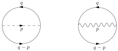
Figure 1: Hartree-Fock approximation to $\Omega_{2}(G,\Delta,D)$. The solid, dash and wavy lines are the nucleon propagator G, the $\sigma$ meson propagator $\Delta$ and the $\omega$ meson propagator $D$ respectively. $q$ and $p$ are the four momenta.

The analytic expression is

$$\Omega_{2}(G,\Delta,D)=\frac{ig_{\sigma}^{2}}{2}\int_{p}\int_{q}Tr\left[G(q)G(q-p)\Delta(p)\right]+\frac{ig_{\omega}^{2}}{2}\int_{p}\int_{q}Tr\left[\gamma^{\mu}G(q)\gamma^{\nu}G(q-p)D_{\mu\nu}(p)\right].$$ (9)

From the stationary condition (2) which demands that $\Omega(G,\Delta,D)$ be stationary against variations of $G$, $\Delta$ and $D$ respectively, we will have the following gap equations

$$G(q)^{-1} = G_{0}(q)^{-1}+g_{\sigma}^{2}\int_{p}G(q-p)\Delta(p)+g_{\omega}^{2}\int_{p}\gamma^{\mu}G(q-p)\gamma^{\nu}D_{\mu\nu}(p),$$ (10)

$$\Delta(p)^{-1} = \Delta_{0}(p)^{-1}-g_{\sigma}^{2}\int_{q}Tr\left[G(q)G(q-p)\right],$$ (11)

$$D_{\mu\nu}(p)^{-1} = D_{0,\mu\nu}(p)^{-1}-g_{\omega}^{2}\int_{q}Tr\left[\gamma_{\mu}G(q)\gamma_{\nu}G(q-p)\right].$$ (12)

The above equations can be also represented pictorially in Fig.2.

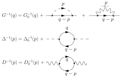
Figure 2: The gap equations satisfied by the nucleon, the $\sigma$ meson and the $\omega$ meson propagators at Hartree-Fock approximation. $q$ and $p$ are the four momenta.

These integration equations are nonlinear coupled and momentum dependent. Needless to say they are very difficult for computation. The certain approximations should be adopted.

III solving gap equations and thermodynamic potential

In this section we will solve the gap equations through certain approximations. The thermodynamic potential will be consistently determined. Then we will derive the pressure and the net baryon density and demonstrate how the thermodynamical consistency is achieved.

To solve the equations, we need first to decouple the equations. As in usual Hartree or Hartree-Fock approximation in studying the nuclear matter, the meson propagators are treated as the free propagators d . In this paper, as the first step, we will simplify the equations by replacing the meson propagators by the free ones. This also means we have neglected the medium effects to the mesons. We expect that under this approximation it could yield the results which are consistent with those of the MFT. The approximation means

$$\Delta(p)=\Delta_{0}(p),\ \ \ \ D_{\mu\nu}(p)=D_{0,\mu\nu}(p).$$ (13)

As a result the thermodynamic potential is reduced to

$$\Omega(G,\Delta_{0},D_{0})= i \int_{p}\ln G_{0}(p)G^{-1}(p)+i\int_{p}\left[G_{0}^{-1}(p)G(p)-1\right]$$ (14)

$$+ \frac{ig_{\sigma}^{2}}{2}\int_{p}\int_{q}Tr\left[G(q)G(q-p)\Delta_{0}(p)\right]+\frac{ig_{\omega}^{2}}{2}\int_{p}\int_{q}Tr\left[\gamma^{\mu}G(q)\gamma^{\nu}G(q-p)D_{0,\mu\nu}(p)\right].$$

The gap equations are much simplified accordingly. Only the nucleon gap equation (10) is left and needs to be solved. To proceed we take the following ansatz of the full nucleon propagator

$$G(q)=\frac{i}{\gamma_{\mu}q^{\mu}-m_{N}+\Sigma},$$ (15)

where $\Sigma$ is the proper nucleon self-energy which will be determined by the equation (10). It can be generally written as

$$\Sigma(q)=\Sigma_{s}(q)-\gamma^{0}\Sigma_{0}(q)+{\bm{\gamma}}{\bm{\cdot}}{\bf q}\Sigma_{v}(q).$$ (16)

Thus we can define an effective nucleon mass

$$M_{N}(q)=m_{N}-\Sigma_{s}(q),$$ (17)

which is momentum dependent. As the nuclear matter is a uniform system at rest, the $\Sigma_{v}$ term in equation (16) is usually neglected as in RHA calculation c . In the usual HF approximation in the study of the nuclear matter, the contribution of the $\Sigma_{v}$ term to the final physical result is also found to be very small d . In our discussion this term will be neglected. Substituting equations (15) and (16) into equation (10), after some calculations on separating the terms which are associated with and without $\gamma$ matrix, and then by comparing the two sides of the equation, we can obtain the following equations for the components of $\Sigma$

$$\Sigma_{s}(q)=ig_{\sigma}^{2}\int_{p}\frac{-M_{N}(q)}{\left[(q_{0}^{*}-p_{0})^{2}-E_{\bf q-p}^{2}\right]\left[p_{0}^{2}-E_{\sigma}({\bf p})^{2}\right]}+ig_{\omega}^{2}\int_{p}\frac{4M_{N}(q)}{\left[(q_{0}^{*}-p_{0})^{2}-E_{\bf q-p}^{2}\right]\left[p_{0}^{2}-E_{\omega}({\bf p})^{2}\right]},$$ (18)

$$\Sigma_{0}(q)=ig_{\sigma}^{2}\int_{p}\frac{q_{0}^{*}-p_{0}}{\left[(q_{0}^{*}-p_{0})^{2}-E_{\bf q-p}^{2}\right]\left[p_{0}^{2}-E_{\sigma}({\bf p})^{2}\right]}+ig_{\omega}^{2}\int_{p}\frac{2q_{0}^{*}-2p_{0}}{\left[(q_{0}^{*}-p_{0})^{2}-E_{\bf q-p}^{2}\right]\left[p_{0}^{2}-E_{\omega}({\bf p})^{2}\right]},$$ (19)

where $q_{0}^{*}=q_{0}-\Sigma_{0}(q)$, $E_{\sigma/\omega}({\bf p})=\sqrt{{\bf p^{2}}+m_{\sigma/\omega}^{2}}$ and $E_{\bf q-p}=\sqrt{({\bf q-p})^{2}+M_{N}(q)^{2}}$. After we perform the sums over the Matsubara frequencies, we obtain

$$\Sigma_{s}(q) = -g_{\sigma}^{2}\int\frac{d^{3}\bf p}{(2\pi)^{3}}\frac{M_{N}(q)}{2E_{\sigma}({\bf p})E_{\bf q-p}}\left[A_{\sigma}-B_{\sigma}\right]+g_{\omega}^{2}\int\frac{d^{3}\bf p}{(2\pi)^{3}}\frac{2M_{N}(q)}{E_{\omega}({\bf p})E_{\bf q-p}}\left[A_{\omega}-B_{\omega}\right],$$ (20)

$$\Sigma_{0}(q) = g_{\sigma}^{2}\int\frac{d^{3}\bf p}{(2\pi)^{3}}\frac{1}{2E_{\sigma}({\bf p})E_{\bf q-p}}\left[C_{\sigma}-D_{\sigma}\right]+g_{\omega}^{2}\int\frac{d^{3}\bf p}{(2\pi)^{3}}\frac{1}{E_{\omega}({\bf p})E_{\bf q-p}}\left[C_{\omega}-D_{\omega}\right],$$ (21)

where the expressions of $A_{i}$, $B_{i}$, $C_{i}$ and $D_{i}$ ($i=\sigma,\omega$) are given in the following,

$$A_{i}=\frac{n_{i}(q_{0}^{*}-E_{\bf q-p})-\tilde{n}_{+}E_{i}}{(q_{0}^{*}-E_{\bf q-p})^{2}-E_{i}^{2}},\ \ \ \ B_{i}=\frac{n_{i}(q_{0}^{*}+E_{\bf q-p})+\tilde{n}_{-}E_{i}}{(q_{0}^{*}+E_{\bf q-p})^{2}-E_{i}^{2}},$$ (22)

$$C_{i}=\frac{q_{0}^{*}(q_{0}^{*}-E_{\bf q-p})n_{i}-E_{i}^{2}n_{i}-E_{i}E_{\bf q-p}\tilde{n}_{+}}{(q_{0}^{*}-E_{\bf q-p})^{2}-E_{i}^{2}},\ \ \ \ D_{i}=\frac{q_{0}^{*}(q_{0}^{*}+E_{\bf q-p})n_{i}-E_{i}^{2}n_{i}-E_{i}E_{\bf q-p}\tilde{n}_{-}}{(q_{0}^{*}+E_{\bf q-p})^{2}-E_{i}^{2}},$$ (23)

in which $E_{i}=\sqrt{{\bf p}^{2}+m_{i}^{2}}$ and

$$n_{i}=\frac{1}{e^{\beta E_{i}}-1},\ \ \ \ \ \ \tilde{n}_{\pm}=\frac{1}{e^{\beta(E_{\bf q-p}\mp\mu^{*})}+1},$$ (24)

where $\mu^{*}=\mu-\Sigma_{0}(q)$ and $\mu$ is the baryon chemical potential. In obtaining equations (20) and (21), we have encountered the divergent terms which are independent of the distribution functions $n_{i}$ and $\tilde{n}_{\pm}$. In principle these divergent parts could be properly renormalized. However, in this rudimentary work, we simply neglect the divergent parts which are not explicit temperature dependent. This treatment is not strange in the literature p ; u .

Now the equations are finite but momentum dependent, which are still intractable. We note that in studying the nuclear matter, the effective mass is usually defined as the pole of the full propagator in the limit ${\bf q}\to 0$ v ; t . In light of this definition, the effective nucleon mass here can be defined by

$$\left.{q_{0}^{*}}^{2}-{\bf q}^{2}-M_{N}^{2}(|q_{0}^{*}|=M_{N},|{\bf q}|=0)\right|_{|{\bf q}|=0}=0.$$ (25)

This means in equations (20) and (21) we will take $|{\bf q}|=0$ and set $|q_{0}^{*}|=M_{N}$. The treatment is different from the usual pole approximation for that we will take $|{\bf q}|=0$ before the angular integration performed. This will greatly simplify the calculation. Furthermore, as $|q_{0}^{*}|=M_{N}$, $q_{0}^{*}$ can be set to either positive or negative value. In order to ensure that at $\mu=0$ the baryon density keeps zero which can be realized in our later discussion, here we will take $q_{0}^{*}=M_{N}$ in $A_{i}$ and $B_{i}$, while take $q_{0}^{*}=-M_{N}$ in $C_{i}$ and $D_{i}$. After these approximations and treatments, the equations (20) and (21) will be further simplified to

$$\Sigma_{s}=-g_{\sigma}^{2}\int\frac{d^{3}\bf p}{(2\pi)^{3}}\frac{M_{N}}{2E_{\sigma}E}\frac{2(M_{N}-E)n_{\sigma}-E_{\sigma}(\tilde{n}_{+}+\tilde{n}_{-})}{(M_{N}-E)^{2}-E_{\sigma}^{2}}+g_{\omega}^{2}\int\frac{d^{3}\bf p}{(2\pi)^{3}}\frac{2M_{N}}{E_{\omega}E}\frac{2(M_{N}-E)n_{\omega}-E_{\omega}(\tilde{n}_{+}+\tilde{n}_{-})}{(M_{N}-E)^{2}-E_{\omega}^{2}},$$ (26)

$$\Sigma_{0}=g_{\sigma}^{2}\int\frac{d^{3}\bf p}{(2\pi)^{3}}\frac{-(\tilde{n}_{+}-\tilde{n}_{-})}{2(M_{N}-E)^{2}-2E_{\sigma}^{2}}+g_{\omega}^{2}\int\frac{d^{3}\bf p}{(2\pi)^{3}}\frac{-(\tilde{n}_{+}-\tilde{n}_{-})}{(M_{N}-E)^{2}-E_{\omega}^{2}},$$ (27)

where $E=\sqrt{{\bf p}^{2}+M_{N}^{2}}$. Now $\Sigma_{s}$, $\Sigma_{0}$ and $M_{N}$ become momentum independent and can be numerically calculated.

In the next we will demonstrate how the thermodynamic potential, the pressure and net baryon density can be derived in a thermodynamical consistent way.

Considering equation (10), (13) and (15) we can have

$$G_{0}(q)^{-1}G(q)-1=i\Sigma(q)G(q),$$ (28)

$$\Sigma(q)=ig_{\sigma}^{2}\int_{p}G(q-p)\Delta_{0}(p)+ig_{\omega}^{2}\int_{p}\gamma_{\mu}G(q-p)\gamma_{\nu}D_{0}^{\mu\nu}(p).$$ (29)

Substituting the above equations into equation (14), the thermodynamic potential will be reduced to

$$\Omega=i\int_{p}\ln G_{0}(p)G(p)^{-1}-\frac{1}{2}\int_{q}Tr\left[G(q)\Sigma(q)\right].$$ (30)

The pressure can be obtained by the thermodynamic relation

$$P=-\Omega.$$ (31)

For the consistency of the calculation under our approximation, $\Sigma(q)$ in equation (30) will be also determined at $|{\bf q}|=0$ and $|q_{0}^{*}|=M_{N}$, which means $\Sigma$ becomes independent of the momentum in equation (30). After the frequency sums in equation (30) and considering equation (31) we can obtain the pressure as

$$P(\mu,T)=\frac{4}{3}\int\frac{d^{3}\bf p}{(2\pi)^{3}}\frac{\bf{p}^{2}}{E}\left[\frac{1}{e^{\beta(E-\mu^{*})}+1}+\frac{1}{e^{\beta(E+\mu^{*})}+1}\right]-2M_{N}\Sigma_{s}\int\frac{d^{3}\bf p}{(2\pi)^{3}}\frac{1}{E}\left[\frac{1}{e^{\beta(E-\mu^{*})}+1}+\frac{1}{e^{\beta(E+\mu^{*})}+1}\right]$$ (32)

$$+2\Sigma_{0}\int\frac{d^{3}\bf p}{(2\pi)^{3}}\left[\frac{1}{e^{\beta(E-\mu^{*})}+1}-\frac{1}{e^{\beta(E+\mu^{*})}+1}\right],$$

where $\Sigma_{s}$ and $\Sigma_{0}$ are determined by solving equations (26) and (27). In (32) we have also neglected the divergent terms which are independent of the distribution functions.

The thermodynamical consistency requires that at fixed $T$ and $\mu$ the pressure will be maximized with respect to $\Sigma_{s}$ or $\Sigma_{0}$, when $\Sigma_{s}$ and $\Sigma_{0}$ are independent variables. This requirement will be satisfied by the stationary condition in the CJT formalism. To make it clear, we assume that $P$ is still in its functional form of $G$, then from equation (15), which indicates $G$ is a function of $\Sigma$, and considering the stationary condition (2) we will have

$$\frac{dP(G(\Sigma))}{d\Sigma}=\frac{dP(G(\Sigma))}{dG}\frac{dG(\Sigma)}{d\Sigma}=0.$$ (33)

This equation ensures the thermodynamical consistency. So when the pressure or the thermodynamic potential is self-consistently determined by solving the gap equations, which are derived by the stationary conditions, the thermodynamical consistency will be automatically achieved. However, one should notice that the pressure in the form of equation (32) can not be maximized with respect to $\Sigma_{s}$ or $\Sigma_{0}$, because in obtaining equation (32), the gap equations have been already substituted into it, which makes that $\Sigma_{s}$ and $\Sigma_{0}$ are not independent variables in equation (32).

Next we will derive the net baryon density of the system. The density will be determined by the thermodynamic relation

$$\rho=\left.\frac{\partial P}{\partial\mu}\right|_{T}.$$ (34)

From a general expression of the pressure, which is a function of the independent variables $T$, $\mu$ and $\Sigma$, we can write down the partial derivative in the following expression

$$\left.\frac{\partial P(\Sigma,\mu,T)}{\partial\mu}\right|_{T}=\left.\frac{\partial P(\Sigma,\mu,T)}{\partial\mu}\right|_{\Sigma,T}+\left.\frac{\partial P(\Sigma,\mu,T)}{\partial\Sigma}\right|_{\mu,T}\left.\frac{\partial\Sigma}{\partial\mu}\right|_{T}.$$ (35)

According to equation (33) the second term on the r.h.s of equation (35) becomes to zero, which shows a fulfillment of the thermodynamical consistency. The partial derivative is reduced to

$$\left.\frac{\partial P(\Sigma,\mu,T)}{\partial\mu}\right|_{T}=\left.\frac{\partial P(\Sigma,\mu,T)}{\partial\mu}\right|_{\Sigma,T}.$$ (36)

Then from equation (14) and considering equation (31), the derivative can be formally evaluated as

$$\left.\frac{\partial P(\Sigma,\mu,T)}{\partial\mu}\right|_{T} = -i\frac{\partial}{\partial\mu}\int_{p}\ln\left[G_{0}(p)G(p)^{-1}\right]+\int_{q}Tr\left[\frac{\partial G(q)}{\partial\mu}\Sigma(q)\right]$$ (37)

$$- \int_{q}Tr\left\{\frac{\partial G(q)}{\partial\mu}\left[ig_{\sigma}^{2}\int_{p}G(q-p)\Delta_{0}(p)+ig_{\omega}^{2}\int_{p}\gamma_{\mu}G(q-p)\gamma_{\nu}D_{0}^{\mu\nu}(p)\right]\right\}.$$

From equation (29) we find that the second term and third term on r.h.s of equation (37) will cancel each other, thus the final result is

$$\left.\frac{\partial P(\Sigma,\mu,T)}{\partial\mu}\right|_{T}=-i\frac{\partial}{\partial\mu}\int_{p}\ln\left[G_{0}(p)G(p)^{-1}\right].$$ (38)

Then the net baryon density is given as

$$\rho=4\int\frac{d^{3}\bf p}{(2\pi)^{3}}\left[\frac{1}{e^{\beta(E-\mu^{*})}+1}-\frac{1}{e^{\beta(E+\mu^{*})}+1}\right].$$ (39)

This is the standard form of net density for quasi-particles, which also indicates that the thermodynamic functions could be calculated thermodynamical consistently.

Furthermore the energy density of the system can be derived by

$$\varepsilon=-P+\mu\rho+T\frac{\partial P}{\partial T}.$$ (40)

In the following we can study the thermodynamics of the nuclear matter.

IV numerical results and comparison to MFT

The coupling constants $g_{\sigma}$ and $g_{\omega}$ will be refitted by reproducing the correct saturation properties of the nuclear matter at zero temperature. The nucleon mass, sigma meson mass and omega meson mass are taken as $m_{N}=939MeV$, $m_{\sigma}=550MeV$ and $m_{\omega}=783MeV$. By setting $T=0$, from equation (32), (39) and (40) we can reproduce the correct binding energy curve of the nuclear matter which means at a saturation density of $0.16$ nucleons per $fm^{3}$ it has a binding energy of $16MeV$ per nucleon. The curve of energy per nucleon versus density is shown in Fig.3. The coupling constants thus are fixed at $g_{\sigma}^{2}=155.6$ and $g_{\omega}^{2}=521.5$. These values look a little greater than those of the MFT which are $g_{\sigma}^{2}=91.6$ and $g_{\omega}^{2}=136.2$ d .

Figure 3: The average energy per nucleon minus the nucleon mass $m_{N}$ as functions of baryon density at zero temperature in the CJT formalism (solid line) and MFT (dashed line).

Figure 4: The nuclear matter equations of state at zero temperature in the CJT formalism (solid line) and MFT (dashed line).

The binding energy curve of MFT is also plotted in Fig.3 in dashed line. We can see that the result of CJT is very close to that of MFT. At low density the energy curve of CJT is almost overlap with the energy curve of MFT; at high density the curve of CJT rises a little slower than that of MFT. The compressibility of nuclear matter at saturation density calculated in the CJT formalism turns out to be

$$K\equiv p_{F}^{2}\frac{d^{2}(\varepsilon/\rho)}{dp_{F}^{2}}=485MeV,$$ (41)

where $p_{F}$ is the Fermi momentum. It is smaller compared to that of the MFT which is $K=540MeV$. The equation of state $P$ vs. $\varepsilon$ for nuclear matter is shown in Fig.4. The CJT and MFT results are almost overlap. Note the approach from below to the casual limit $\varepsilon=P$ (where $c_{sound}=c_{light})$ at high density.

Figure 5: The effective nucleon mass as functions of temperature at zero density in the CJT formalism (solid line) and MFT (dashed line).

Figure 6: The isotherms of $P$ vs. $\rho$ at $T=10MeV$ and $T=15MeV$ in the CJT formalism (solid line) and MFT (dashed line).

At finite temperature, from equation (17) and considering (25), the effective nucleon mass as a function of temperature at zero density can be plotted in Fig.5 (solid line). When compared to that of MFT (dashed line), the effective mass from the CJT calculation drops a little more slowly at high temperature. The well-known liquid-gas phase transition of the nuclear matter at low temperature also exists by the CJT calculation. The isotherms of $P$ vs. $\rho$, which show the first order transitions, are plotted in Fig.6. The CJT results are again found very close to the MFT results. The critical temperature in the CJT calculation is about $19MeV$ which is almost the same as that in the MFT.

V summary

In this paper we have made an attempt to use the CJT formalism to study the nuclear matter. As the first step, we have neglected the medium effects to the mesons and obtained the results which are found very consistent with those from MFT. We have also demonstrated how the thermodynamical consistency has been achieved in the CJT formalism in studying the nuclear matter. In our discussion one can also see that the beyond mean field calculation of the nuclear matter can be carried out in the CJT formalism, at least by including the medium effects to the mesons. However it is obvious that the calculation will be quite involved. This topic will be studied in our further work.

- (1) B.D. Serot, J.D. Walecka, Int.J.Mod.Phys. E6 (1997) 515, nucl-th/9701058.
- (2) R.J. Furnstahl, B.D. Serot, Comments Nucl.Part.Phys. 2 (2000) A23, nucl-th/0005072.
- (3) B.D. Serot, Rep.Prog.Phys. 55 (1992) 1855.
- (4) J.D. Walecka, Theoretical Nuclear and Subnuclear Physics, Oxford Univ. Press, 1995.
- (5) S.A. Chin, Ann.Phys. 108 (1977) 301.
- (6) B.D. Serot, J.D. Walecka, Adv.Nucl.Phys. 16 (1986) 1.
- (7) A.L. Fetter, J.D. Walecka, Quantum Theory of Many-Particle System, McGraw-Hill, 1971.
- (8) C.J. Horowitz, B.D. Serot, Nucl.Phys. A399 (1983) 529.
- (9) R.J. Furnstahl, R.J. Perry, B.D. Serot, Phys.Rev. C40 (1989) 321.
- (10) R. Jackiw, Phys.Rev. D9 (1974) 1689.
- (11) L. Dolan, R. Jackiw, Phys.Rev. D9 (1974) 3320.
- (12) S. Coleman, E. Weinberg, Phys.Rev. D7 (1973) 1888.
- (13) L. Dolan, R. Jackiw, Phys.Rev. D9 (1974) 2904.
- (14) A. Linde, Rep.Prog.Phys. 42 (1979) 390.
- (15) J. Cornwall, R. Jackiw, E. Tomboulis, Phys.Rev. D10 (1974) 2428.
- (16) G. Amelino-Camelia, So-Young Pi, Phys.Rev. D47 (1993) 2356.
- (17) G. Amelino-Camelia, Phys.Rev. D49 (1994) 2740.
- (18) P. Nicholas, J.Phys. G25 (1999) 2225.
- (19) A. Barducci, R. Casalbuoni, etc., Phys.Rev. D38 (1988) 238.
- (20) A. Barducci, R. Casalbuoni, etc., Phys.Rev. D49 (1994) 426.
- (21) J.-S. Cheng, P.-F. Zhuang, J.-R. Li, Phys.Rev. C68 (2003) 045209-1.
- (22) J. Kapusta, Finite-Temperature Field Theory, Cambridge Univ. Press, 1989.
- (23) A. Ayala, P. Amore, A. Aranda, Phys.Rev. C66 (2002) 045205.
- (24) S. Gao, Y.-J. Zhang, R.-K. S, Phys.Rev. C52 (1995) 380.
- (25) C. Song, Phys.Rev. D48 (1993) 1375.