New inversion methods for the Lorentz Integral Transform

Abstract

The Lorentz Integral Transform approach allows microscopic calculations of electromagnetic reaction cross sections without explicit knowledge of final state wave functions. The necessary inversion of the transform has to be treated with great care, since it constitutes a so-called ill-posed problem. In this work new inversion techniques for the Lorentz Integral Transform are introduced. It is shown that they all contain a regularization scheme, which is necessary to overcome the ill-posed problem. In addition it is illustrated that the new techniques have a much broader range of application than the present standard inversion method of the Lorentz Integral Transform.

I Introduction

About a decade ago the Lorentz Integral Transform (LIT) method has been proposed in order to perform ab initio calculations of electroweak reactions with nuclei into the continuum LIT . The great advantage of the method lies in the fact that a calculation of continuum wave functions is not necessary. Indeed the LIT approach reduces a continuum state problem to a bound-state like problem and thus it is sufficient to use bound-state methods. Hence it is not surprising that the LIT method has been applied to microscopic calculations of quite a few electroweak cross sections of various nuclei ranging from A=2-7: inclusive electron scattering (see e.g. PRL1 ; ELOT04 ), total photoabsorption cross sections (see e.g. PRL2 ; PRL3 ; Sonia ), exclusive electromagnetic reactions Lapiana ; Sofia , photomeson production Christoph , and weak processes Nir . The list of application shows that the LIT approach has proven to be an important progress opening up the possibility to carry out microscopic calculations not only for reactions of classical few-body systems (deuteron, three-body nuclei), but also for reactions of more complex nuclei.

The LIT method proceeds in two steps. First one calculates an integral transform of the searched function $R(\omega)$ with a Lorentzian-shape kernel:

$$L(\sigma_{\rm R},\sigma_{\rm I})=\int d\omega{\frac{R(\omega)}{(\omega-\sigma_{\rm R})^{2}+\sigma_{\rm I}^{2}}}\,,\,\,\,\,\,\,\,\,\,\,\sigma_{\rm R}\,,\sigma_{\rm I}>0\,.$$ (1)

Then, in a second step, one inverts the obtained integral transform. The inversion, however, is in principle an ill-posed problem and the resulting consequences were already discussed in FBS . In order to introduce the reader to the problem we summarize the main points of that discussion. The inversion of (1) is unstable with respect to high frequency oscillations $\Omega$. Adding such a high-frequency term $\Delta_{\Omega}R(\omega)$ to $R(\omega)$ leads to an additional $\Delta_{\Omega}L(\sigma_{\rm R},\sigma_{\rm I})$ in the transform. With growing $\Omega$ on the one hand and a constant non negligible oscillation amplitude $\Delta_{\Omega}R$ on the other hand $\Delta_{\Omega}L$ becomes increasingly small and might become even smaller than the size of errors in the calculation. Thus $\Delta_{\Omega}R$ could not be discriminated. If one reduces the error in the calculation one can push the not discriminated $\Delta_{\Omega}R$ to higher and higher $\Omega$. However, even if the excluded frequency range is physically unimportant, one cannot simply find a solution of the response by application of the inverse operator, since the unphysical oscillations cannot be separated from the solution. As further explained in FBS one then has to use a regularization scheme for the inversion in order to avoid such problems. Therefore a specific inversion method with a built-in regularization was recommended. In fact this method has been used in all the above mentioned LIT calculations leading to very safe inversion results. On the other hand in all these calculations the various LITs have (i) a rather simple structure, where essentially only a single peak of $R(\omega)$ has to be resolved or (ii) a more complicated structure, which however could be subdivided in a sum of simply structured responses, where the various LITs have been inverted separately. Case (ii) was already encountered in LIT , where the inclusive longitudinal deuteron electron response $R(\omega)$ was calculated at a constant momentum transfer. There it was necessary to separate out the Coulomb monopole and quadrupole transitions, which lead to a shoulder of the corresponding $R(\omega)$ at the break-up threshold, while the rest of the response shows the typical quasi-elastic peak structure. Obviously it would be advantageous to invert the total LIT by just one inversion with a method appropriated for more complicated structures. In addition it is not guaranteed that one can always make the above subdivision in a sum of simply structured responses, e.g. in case of two rather close peaks in the same multipole transition. In such cases the standard inversion method would not be sufficiently precise.

The aim of the present paper is twofold. The main purpose is the investigation of the problem of the inversion of a more structured $R(\omega)$ and to introduce alternative inversion methods. As already pointed out the LIT method reduces a continuum state problem to a bound-state like problem, which can be solved with typical bound-state techniques. In recent years many different solutions for the bound-state problem of nuclei with $A>3$ have been developed as illustrated for example in a rather recent paper about the ⁴He ground-state solution with a realistic nucleon-nucleon potential, where seven different theoretical methods were applied He4 . Many of these methods could also be used for a LIT calculation and as a second aim we want to show to potential future practitioners of the LIT method that reliable inversion techniques exist even in case of more structured response functions.

The paper is organized as follows. In section II we give a brief outline of the LIT approach. The standard inversion method and alternative approaches are described in section III. Results with the various inversion techniques are discussed in section VI.

II The Lorentz Integral Transform method

In this section we give a brief outline of the LIT technique discussing however the approach for inclusive reactions only. The calculation of exclusive reactions is somewhat more complicated, but one proceeds in principle in a very similar manner Lapiana ; Sofia .

As pointed out in the introduction the starting point of the LIT method LIT is the calculation of the integral transform of $R(\omega)$ given in eq. (1). The function $R$ depends on the internal excitation energy $\omega=E_{f}-E_{0}$ of a given particle system and contains information about the transition of the system from the ground state $|\Psi_{0}\rangle$, with energy $E_{0}$, to the final states $|\Psi_{f}\rangle$, with energy $E_{f}$, induced by an external probe. In case of an inclusive reaction $R(\omega)$ denotes the response function

$$R(\omega)=\int d\Psi_{f}|\langle\Psi_{f}|\hat{O}|\Psi_{0}\rangle|^{2}\delta(E_{f}-E_{0}-\omega)\,,$$ (2)

where $\hat{O}$ is a transition operator which characterizes the specific process under consideration. The response function and in principle also the LIT are observable quantities. However, in experiment $R(\omega)$ can be determined more directly, while $L(\sigma_{\rm R},\sigma_{\rm I})$ is only accessible via the explicit integration (1) of an experimentally over a sufficiently large $\omega$-range determined $R(\omega)$. Thus also in a theoretical calculation it is preferable to eventually determine $R(\omega)$. The key point of the LIT method is nonetheless a direct calculation of $L(\sigma_{\rm R},\sigma_{\rm I})$, i.e. without explicit knowledge of $R(\omega)$. Only in a second step $R$ is obtained from the inversion of the transform. The great advantage of the method lies in the fact that the generally very complicated calculation of final state wave functions $|\Psi_{f}\rangle$ can be avoided as will be discussed below. On the contrary a conventional calculation of $R(\omega)$ can only be carried out with the explicit knowledge of $|\Psi_{f}\rangle$.

Given an Hamiltonian $H$ of the particle system under consideration one may use the completeness of the eigenstates of $H$ to show that $L(\sigma_{\rm R},\sigma_{\rm I})$ is determined via the following differential equation LIT

$$(H-E_{0}-\sigma^{*})|\tilde{\Psi}\rangle=\hat{O}|\Psi_{0}\rangle$$ (3)

with

$$\sigma=\sigma_{\rm R}+i\sigma_{\rm I}\,.$$ (4)

Since $H$ has a real eigenvalue spectrum the corresponding homogeneous differential equation has only the trivial solution. Thus the solution of (3) is unique. This solution leads directly to the transform, in fact one finds

$$L(\sigma_{\rm R},\sigma_{\rm I})=\langle\tilde{\Psi}|\tilde{\Psi}\rangle\,.$$ (5)

Different from a Schrödinger equation at positive energies one has a very simple boundary condition for the solution of (3). Due to the localized source at the right hand side of (3) and because $\sigma$ is complex, $\tilde{\Psi}$ vanishes at large distances similar to a bound-state wave function. Therefore one can apply similar techniques as for the calculation of a bound-state wave function. It is evident that the much more complicated continuum state problem is completely avoided by the LIT method.

III Inversion methods for the Lorentz Integral Transform

In order to invert the LIT one has to calculate $L(\sigma_{\rm R},\sigma_{\rm I})$ for a set of $\sigma_{\rm R}$ values at fixed $\sigma_{\rm I}>0$. If one wants to determine $R(\omega)$ in a range $\omega_{\rm min}\leq\omega\leq\omega_{\rm max}$ one should choose $\sigma_{\rm R}$ in the interval $\omega_{\rm min}-\sigma_{\rm I}\leq\sigma_{\rm R}\leq\omega_{\rm max}+\sigma_{\rm I}$. For such $\sigma_{\rm R}$ values the kernel in (1) takes a resonant form with the width determined by $\sigma_{\rm I}$. The principal difficulties of the LIT inversion were already discussed in the introduction, hence in the following subsections we directly describe the standard LIT inversion method (subsection A) and the new inversion approaches (subsections B-D).

III.1 Inversion with a set of basis functions

The present standard LIT inversion method consists in the following ansatz for the response function

$$R(\omega^{\prime})=\sum_{n=1}^{N}c_{n}\chi_{n}(\omega^{\prime},\alpha_{i})\,$$ (6)

with $\omega^{\prime}=\omega-\omega_{\rm th}$, where $\omega_{\rm th}$ is the threshold energy for the break-up into the continuum. The $\chi_{n}$ are given functions with nonlinear parameters $\alpha_{i}$. A basis set frequently used in the LIT calculations of [1-11] is

$$\chi_{n}(\omega,\alpha_{i})=\omega^{\alpha_{1}}\exp(-{\frac{\alpha_{2}}{n\omega}})\,.$$ (7)

In addition also possible information on narrow levels, like e.g. elastic transitions, could be incorporated easily into the set $\chi_{n}$.

Substituting such an expansion into the right hand side of (1) one obtains

$$L(\sigma_{\rm R},\sigma_{\rm I})=\sum_{n=1}^{N}c_{n}\tilde{\chi}_{n}(\sigma_{\rm R},\sigma_{\rm I},\alpha_{i})\,,$$ (8)

where

$$\tilde{\chi}_{n}(\sigma_{\rm R},\sigma_{\rm I},\alpha_{i})=\int_{0}^{\infty}d\omega^{\prime}{\frac{\chi_{n}(\omega^{\prime},\alpha_{i})}{(\omega^{\prime}-\sigma_{\rm R})^{2}+\sigma_{\rm I}^{2}}}\,\,.$$ (9)

For given $\alpha_{i}$ the linear parameters $c_{n}$ are determined from a best fit of $L(\sigma_{\rm R},\sigma_{\rm I})$ of eq. (8) to the calculated $L(\sigma_{\rm R},\sigma_{\rm I})$ of eq. (5) for a number of $\sigma_{\rm R}$ points much larger than $N$. If one takes the basis set (7) one should vary the nonlinear parameter $\alpha_{2}$ in a rather large range, while one can determine $\alpha_{1}$ from the possibly known threshold behaviour of $R$ or one can vary $\alpha_{1}$ within a reasonable range.

For any values of $N$, $\alpha_{1}$, and $\alpha_{2}$ the overall best fit is selected and then the procedure is repeated for $N=N+1$ till a stability of the inverted response is obtained and taken as inversion result. A further increase of $N$ will eventually reach a point, where the inversion becomes unstable leading typically to random oscillations. The reason is that $L(\sigma_{\rm R},\sigma_{\rm I})$ of eq. (8) is not determined precisely enough so that a randomly oscillating $R(\omega)$ leads to a better fit than the true response. It is evident that the number of functions $N$ plays the role of a regularization parameter and has to be chosen within the above mentioned stability region. Normally such a stability region is reached without greater problems, however, it can in principle happen that one does not find a stable result. Then one can either try to improve the precision of the calculated $L(\sigma_{\rm R},\sigma_{\rm I})$ or use different basis sets. In case that the response exhibits an unexpected structure it is useful to decrease the parameter $\sigma_{\rm I}$ in order to have a better resolution in the transform.

We should mention that the completeness of the basis set $\chi_{n}$ is not really relevant. In fact any basis set is only used up to a relatively low value of $N$. Information which can be parametrized only via $\chi_{n}$ with $n>N$ is lost anyway. Therefore it is important to work with a basis set, where a relatively small $N$ leads to a high-quality result of $R(\omega)$. Because of the variation of the nonlinear parameters $\alpha_{i}$ of $\chi_{n}$ many different basis sets are used and it is normally no problem to find a proper basis set.

As already pointed out the standard LIT inversion method leads to high-precision results in case of simply structured response functions, but can have problems in case of more complicated structures. If one considers however just the low-energy part of the response the standard method is very reliable. This is due to the fact that the break-up threshold $\omega_{\rm th}$ is directly incorporated in the inversion ($R(\omega)$ = 0 for $\omega\leq\omega_{\rm th})$ and also a known low-energy behaviour can be directly implemented (e.g. by the parameter $\alpha_{1}$ in (7)). In addition the inversion can be restricted to a small energy interval above threshold avoiding problems arising from structures at higher energies (see also Diego ).

III.2 Inversion with wavelets

The inversion with wavelets is formally very similar to the inversion with a set of basis functions described in the preceding subsection. One starts from the same expansion (6), but one uses wavelets instead of the basis functions $\chi_{n}$. Here we will take the Mexican hat wavelet

$$\varphi(x)=(1-x^{2})~{}\exp(-{\frac{x^{2}}{2}})\,,$$ (10)

which is shown in fig. 1. We expand $R(\omega)$ in the range $\omega_{\rm th}\leq\omega\leq\omega_{\rm max}$ as follows

$$R(\omega)=\sum_{m=0}^{M}\sum_{n=1}^{N_{m}}c_{m,n}\varphi_{m,n}(\omega,\alpha)$$ (11)

with

$$\varphi_{m,n}(\omega,\alpha)=\varphi(\alpha\frac{\omega-\omega_{m,n}}{2^{m}})\,,$$ (12)

where $\alpha$ is a nonlinear parameter and the $N_{m}$ grid points $\omega_{m,n}$ are equally distributed ($\omega_{m,n}=n(\omega_{\rm max}-\omega_{\rm th})/(N_{m}+1))$. Such an expansion leads to the following LIT

$$L(\sigma_{\rm R},\sigma_{\rm I})=\sum_{m=0}^{M}\sum_{n=1}^{N_{m}}c_{m,n}\tilde{\varphi}_{m,n}(\sigma_{\rm R},\sigma_{\rm I},\alpha)$$ (13)

with

$$\tilde{\varphi}_{m,n}(\sigma_{\rm R},\sigma_{\rm I},\alpha)=\int_{\omega_{\rm th}}^{\infty}d\omega{\frac{\varphi_{m,n}(\omega,\alpha)}{(\omega-\sigma_{\rm R})^{2}+\sigma_{\rm I}^{2}}}\,\,.$$ (14)

The wavelets $\varphi_{m,n}$ are strongly localized functions about $\omega=\omega_{m,n}$ in contrast to the basis functions $\chi_{n}$ in subsection A, which generally are considerably different from zero over a rather large $\omega$-range. The widths of the wavelets can be modified with the parameter $\alpha$. In addition with the parameter $M$ one can choose the presence of various scales of wavelets. Because of these wavelet characteristics one easily understands that they are much more appropriated to represent complicated structure of $R(\omega)$ than the basis functions $\chi_{n}$ of the previous subsection.

For the actual inversion problems discussed in the next section we use up to three different wavelet scales and various values for the $N_{m}$ sets (see table I), in addition we include an additional basis function $\varphi_{0}$, namely a constant ($\varphi_{0}=c_{0}$). For any of the 25 $N_{m}$ sets of table I we proceed as follows. The nonlinear parameter $\alpha$ is varied over a wide range and for any value of $\alpha$ a best fit is performed leading to the determination of the linear parameters $c_{m,n}$. For any $N_{m}$ set the overall best fit is then chosen. Of these 25 inversion results we choose again the overall best fit. In case that unrealistic oscillations are present in the inversion the next best inversion result is taken. Of course such a procedure is nothing else than a regularization scheme.

Table 1: $M$ and $N_{m}$ values used for the wavelet inversion of section IV

						$M$=0
$N_{0}$	15	31	63	127	255
						$M$=1
$N_{0}$	7	15	31	63	127	255	15	31	63	127	255
$N_{1}$	7	15	31	63	127	255	7	15	31	63	127
						$M$=2
$N_{0}$	7	15	31	63	127	31	63	127	255
$N_{1}$	7	15	31	63	127	15	31	63	127
$N_{2}$	7	15	31	63	127	7	15	31	63

III.3 Fridman approach applied to the LIT inversion

The following method to invert the Lorentz integral transformation is based on the approach of V. M. Fridman fridman56 . This method solves by iteration the Fredholm integral equation of first order

$$F(x)=\int_{a}^{b}\!dy\,K(x,y)\,f(y)\,,$$ (15)

which has a solution and converges in the Hilbert space of square integrable real functions on $[a,b]$ ($L_{2}(a,b)$) if the kernel $K$ is strictly positive definite and symmetric. The iterative equation is given by

$$f_{l+1}(x)=f_{l}(x)+\lambda\,\left[F(x)-\int_{a}^{b}\!dy\,K(x,y)\,f_{l}(y)\right]\quad,\quad l\in\mathbf{N}_{0}$$ (16)

with $f_{0}\in L_{2}(a,b)$ and $0<\lambda<2\lambda_{1}$, where $\lambda_{1}$ is the smallest characteristic number of $K$. Using the spectral theorem it is evident that the iteration of eq. (16) diverges if at least one eigenvalue of $K$ is in $]-\infty,0]$.

To apply this method to the inversion of the Lorentz integral transform

$$L(\sigma_{\rm R},\sigma_{\rm I})=\int_{\omega_{\rm th}}^{\infty}\!d\omega K(\sigma_{\rm R},\sigma_{\rm I},\omega)R(\omega)\quad,\quad K(\sigma_{\rm R},\sigma_{\rm I},\omega)=\frac{1}{(\omega-\sigma_{\rm R})^{2}+\sigma_{\rm I}^{2}}\quad,\quad\sigma_{\rm I}>0$$ (17)

one has to discretisize the integration and symmetrize the integral kernel $K$. In practice the integration in eq. (17) ranges from $\omega_{\rm th}$ to $\omega_{\rm max}+\sigma_{\rm I}$, since contributions beyond $\omega_{\rm max}+\sigma_{\rm I}$ are of minor importance. The numerical integration is done using the simple formula:

$$\int_{a}^{b}\!dx\,f(x) = \sum_{i=0}^{n}w_{i}\,f(x_{i})\,,$$ (18)

$$h = \frac{b-a}{n}\,,\quad w_{0}=w_{n}=\frac{h}{2}\,,\quad w_{i}=h\,,\quad i\in\{1,\ldots,n-1\}\,,$$

$$x_{i} = a+h\,i\,,\quad i\in\{0,\ldots,n\}\quad.$$

Therefore the symmetrized iterative equation is given by:

$$R_{l+1}(x_{i}) = R_{l}(x_{i})+\lambda\,\left[w_{i}L(x_{i},\sigma_{\rm I})-\sum_{j=0}^{n}K_{ij}^{(\sigma_{\rm I})}R_{l}(x_{j})\right]\,,$$ (19)

$$K_{ij}^{(\sigma_{\rm I})} = \frac{w_{i}w_{j}}{(x_{i}-x_{j})^{2}+\sigma_{\rm I}^{2}}\longleftarrow K(x_{i},\sigma_{\rm I},x_{j})\,,$$ (20)

where $\sigma_{\rm R}$ and $\omega$ lie on the same grid $(x_{i})$. We do not prove that $K_{ij}^{(\sigma_{\rm I})}$ is strictly positive definite, since the algorithm has to diverge if this is not the case and we have to check the convergence numerically anyway.

The iteration is started with the initial function

$$R_{0}(x)=\frac{\sigma_{\rm I}}{\pi}\,L(x,\sigma_{\rm I})\,,$$ (21)

which is motivated by the following definition of the Dirac-Delta-function

$$\delta(x)=\lim_{\sigma_{\rm I}\to 0}\frac{\sigma_{\rm I}}{\pi}\,\frac{1}{x^{2}+\sigma^{2}_{\rm I}}\,.$$ (22)

Let us remind that extracting $R$ using the limit $\displaystyle{{\sigma_{\rm I}\to 0}}$, i.e.

$$R(\sigma_{\rm R})=\lim_{\sigma_{\rm I}\to 0}\frac{\sigma_{\rm I}}{\pi}\,L(\sigma_{\rm R},\sigma_{\rm I})=\lim_{\sigma_{\rm I}\to 0}\frac{\sigma_{\rm I}}{\pi}\,\int_{0}^{\infty}\!d\omega\,K(\sigma_{\rm R},\sigma_{\rm I},\omega)\,R(\omega)\,,$$ (23)

is numerically unstable.

The smallest characteristic number of the integral kernel $\displaystyle{K}$ is the inverse of the largest eigenvalue $\mu_{1}$ of $\displaystyle{(K_{ij}^{(\sigma_{\rm I})})}$. In this work we have used $\lambda=\frac{1}{\mu_{1}}$. This value is not optimized. The larger $\lambda$ is, the faster the algorithm will converge, but the procedure will also become more unstable.

Under real conditions one does not know the solution of the integral equation. One has to compare the “input” Lorentz $L$ with the LIT of the actual result for $R_{l}$. The relative error at every grid point

$$\varepsilon_{l}(x_{i})=\frac{\sum_{j=0}^{n}w_{j}\,K(x_{i},\sigma_{\rm I},x_{j})R_{l}(x_{j})-\,L(x_{i},\sigma_{\rm I})}{L(x_{i},\sigma_{\rm I})}$$ (24)

after $l$ iterations and the mean square sum of $\varepsilon_{l}(x_{i})$ at every grid point

$${\cal E}_{l}=\frac{1}{n^{2}}\sum_{i=0}^{n}\left|\varepsilon_{l}(x_{i})\right|^{2}$$ (25)

is used to check the quality of the iterated solution $R_{l}$ after $l$ recursions. We remind here that this problem is ill-posed and therefore the solution is unstable under perturbation of the input data. With increasing number of iterations the solution will become more and more unstable. Therefore one has always to check whether the result $R_{l}$ is numerically still stable, i.e. free of unphysical oscillations. Solving ill-posed problems requires a regularization scheme. This is naturally provided by this method through the grid $(x_{i})$.

Let us remark at this point that the simple integration formula (eq. (18)) has the advantage that all information entering the inversion process has the same weight except at the boundaries and it has constant grid gap, which provides a constant regularization over the whole integration region. In contrast, a Gauss-Legendre integration grid has smaller grid gaps at the boundaries than in the center of the integration interval leading to a weaker regularization at the boundaries and likely causing a lower quality of the inversion close to threshold. In addition the integration kernel $K$ (eq. (20)) will become more easily numerically singular for the case that $L$ is given on a grid with many points, i.e. more than about $50$ grid points. On the other hand if $L$ is given on a sparse grid, the Gauss-Legendre integration is preferred, since it provides a more precise integration for the same amount of grid points than formula (18). For such a case the mentioned disadvantages of the Gauss-Legendre grid regarding regularization and numerical singularity are not so important any more.

The iteration (19) is stopped if ${\cal E}_{l}$ is smaller than $2.5\cdot 10^{-16}$, if ${\cal E}_{l}$ or $\max_{i\in\{0,1,\dots,n\}}\{\varepsilon_{l}(x_{i})\}$ is increasing or unphysical oscillations arise in the solution. We allow at first some “free” iteration steps, depending on the quality of the input data, before we check if the iteration has to be terminated. This is necessary, since in the first iterations the errors ${\cal E}_{l}$ or $\max_{i\in\{0,1,\dots,n\}}\{\varepsilon_{l}(x_{i})\}$ may increase temporarily due to large initial changes in $R_{l}$.

III.4 Inversion using Banach’s fix point theorem

Let us first consider notations and conventions used in this subsection. We are working in the Hilbert space $L_{2}$ of the square integrable real functions $R(\omega)\equiv\mbox{$\langle\omega|R\rangle$}$ with real arguments $\omega$ which fulfill

$$\int d\omega\,\mbox{$|\omega\rangle$}\mbox{$\langle\omega|$}=1\,\,.$$ (26)

The scalar product and the norm are defined as usual:

$$\mbox{$\langle R_{1}|R_{2}\rangle$}:=\int_{-\infty}^{\infty}d\omega\,\mbox{$\langle R_{1}|\omega\rangle$}\mbox{$\langle\omega|R_{2}\rangle$}\equiv\int_{-\infty}^{\infty}d\omega\,R_{1}(\omega)R_{2}(\omega)\,\,,$$ (27)

and

$$||R||:=\sqrt{\mbox{$\langle R|R\rangle$}}<\infty\,\,.$$ (28)

For a fixed $\sigma_{\rm I}>0$, we are defining the Lorentz integration operator ${\widehat{L}}(\sigma_{\rm I})$ (LIT) in accordance with (1) as follows:

$$\mbox{$\langle\omega|$}{\widehat{L}}(\sigma_{\rm I})\mbox{$|R\rangle$}\equiv L(\omega,\sigma_{\rm I}):=\int d\omega^{\prime}\frac{1}{(\omega-\omega^{\prime})^{2}+\sigma_{\rm I}^{2}}R(\omega^{\prime})\,\,,$$ (29)

where in general, if not noted differently, the upper and lower limit in the integrals is $\infty$ and $-\infty$, respectively. For the inversion method proposed in this subsection, let’s introduce for a fixed Lorentzian $L(\omega,\sigma_{\rm I})$ and a fixed $\sigma_{\rm I}>0$ the following mapping acting on an arbitrary function $R_{1}\in L_{2}$:

$$\mbox{$\langle\omega|$}{\hat{T}}(\sigma_{\rm I},L)\mbox{$|R_{1}\rangle$} =: {\hat{T}}(\sigma_{\rm I},L)(R_{1}(\omega))$$ (30)

$$= \frac{\sigma_{\rm I}}{\pi}L(\omega,\sigma_{\rm I})-\frac{\sigma_{\rm I}}{\pi}\int d\omega^{\prime}\frac{R_{1}(\omega^{\prime})-R_{1}(\omega)}{(\omega^{\prime}-\omega)^{2}+\sigma^{2}_{\rm I}}\,\,.$$

As will be shown in Appendix A.1, this mapping has as fixpoint just the desired response function $R(\omega)$ which creates via (29) the input Lorentzian $L(\omega,\sigma_{\rm I})$:

$${\hat{T}}(\sigma_{\rm I},L)(R(\omega)) = R(\omega)\quad\quad\leftrightarrow$$

$$R(\omega) = \frac{\sigma_{\rm I}}{\pi}L(\omega,\sigma_{\rm I})-\frac{\sigma_{\rm I}}{\pi}\int d\omega^{\prime}\frac{R(\omega^{\prime})-R(\omega)}{(\omega^{\prime}-\omega)^{2}+\sigma^{2}_{\rm I}}\,\,.$$ (31)

Now, in appendix A.2, we will prove with the help of Banach’s Fixpoint Theorem that there exists an $\epsilon>0$ so that for $0<\sigma_{\rm I}<\epsilon$ the series ($n\geq 0$, $R^{(0)}\in L_{2}$ arbitrary)

$$R^{(n+1)}(\omega):={\hat{T}}(\sigma_{\rm I},L)(R^{(n)}(\omega))$$ (32)

has a unique fix point, which is therefore just the searched response $R(\omega)$:

$$R^{(n)}(\omega)\longrightarrow R^{\rm fix}(\omega)\equiv R(\omega)\quad\mbox{for}\quad n\rightarrow\infty\,\,,\quad 0<\sigma_{\rm I}<\epsilon\,\,.$$ (33)

This method works therefore as follows: For a given Lorentzian $L(\omega,\sigma_{\rm I})$ with $\sigma_{\rm I}$ sufficiently small, we choose some arbitrary starting function $R^{(0)}$ (in our practical applications, we have taken always $R^{(0)}=0$ for the sake of simplicity) and then calculate the series (32) till we have reached convergence. The found fixpoint function $R^{\rm fix}$ is then identical with the desired response function $R$. This method is therefore completely parameter free and does not need any suitable basic functions.

In the version discussed so far, this approach has however one serious drawback. Due to the iterative procedure, it is obvious that the fixpoint $R^{\rm fix}$ is a $C^{\infty}$ function, i.e. differentiable up to infinite order. In other words, this method is strictly valid only for response functions which are $C^{\infty}$. The physical response function, however, is not analytic at the threshold energy $\omega_{\rm th}$ of the considered inclusive reaction and is therefore not $C^{\infty}$. In order to get rid of this problem, one has to modify slightly the above discussed algorithm. Instead of the range $]-\infty,\infty[$, all occurring functions $L,R,...$ are now only defined on the interval $[a,b]$, where $a\equiv\omega_{\rm th}$. The upper value $b$ should be in principle $\infty$. However, in practical applications, the Lorentzian $L$, which serves as a input in the algorithm, is known only in some finite range of $\omega$, so that in practice $b$ is not infinite, but still “large”.

Instead of (29) we have therefore to consider

$$L_{(a,b)}(\omega,\sigma_{\rm I}):=\int_{a}^{b}d\omega^{\prime}\frac{1}{(\omega-\omega^{\prime})^{2}+\sigma_{\rm I}^{2}}R(\omega^{\prime})\,\,$$ (34)

and the counterpart of the linear mapping (30) for finite integrals becomes then

$${\hat{T}}_{(a,b)}(\sigma_{\rm I},L)(R_{1}(\omega)) = \frac{\sigma_{\rm I}}{\alpha_{(a,b)}(\omega)}L_{(a,b)}(\omega,\sigma_{\rm I})$$ (35)

$$-\frac{\sigma_{\rm I}}{\alpha_{(a,b)}(\omega)}\int_{a}^{b}d\omega^{\prime}\frac{R_{1}(\omega^{\prime})-R_{1}(\omega)}{(\omega^{\prime}-\omega)^{2}+\sigma^{2}_{\rm I}}$$

with the function

$$\alpha_{(a,b)}(\omega)=\arctan(\frac{\omega-a}{\sigma_{\rm I}})+\arctan(\frac{b-\omega}{\sigma_{\rm I}})\,\,.$$ (36)

The series

$$R_{(a,b)}^{(n+1)}(\omega):={\hat{T}}_{(a,b)}(\sigma_{\rm I},L_{(a,b)}^{R})(R_{(a,b)}^{(n)}(\omega))$$ (37)

has again, as will be shown in appendix A.3, the desired response function $R$ as unique fixpoint for sufficiently small $\sigma_{\rm I}$. So the method works also for functions which are defined only on a finite range.

Summarizing, we have proven that this method allows for not too large $\sigma_{\rm I}$ a unique determination of the response function $R$ for a given Lorentzian $L$. As discussed in section IV in detail, it may however happen in practice that $L$ is not very precisely known, containing for example oscillations due to numerical uncertainties or approximations in its explicit calculation. Therefore, similar to the Fridman approach, also in this method a sort of regularization has to be used in order to avoid resulting unphysical oscillations in $R$. In practice, two numerical tools are used which mutually supplement each other, leading both to a reduction of the numerical resolution. First of all, the number of mesh points in the occurring integrals can be reduced (in analogy to the Fridman method) and second, the total number of iterations should be restricted, for example by choosing a suitable termination condition for ${\cal E}_{l}$ (25).

IV Discussion of results

In the following we apply the various inversion methods of section III to two different cases. First we investigate the efficiency of the regularization procedures implemented in the various inversion methods. As test case we consider a realistic example, where $L(\sigma_{\rm R},\sigma_{\rm I})$ is calculated from eqs. (3,5) without any knowledge of $R(\omega)$. To this end we take $L(\sigma_{\rm R},\sigma_{\rm I})$ from ref. LIT , where the longitudinal response function for inclusive electron scattering off the deuteron at a momentum transfer of $q^{2}=5$ fm^-2 is considered. As described in ref. LIT eq. (3) was solved in an approximate way thus leading to an $L(\sigma_{\rm R},\sigma_{\rm I})$ with a non-negligible error margin. It is evident that for such a case a regularization must be present in the inversion method otherwise reasonable results cannot be obtained. Our second example serves for a different test, namely to check the ability of the various inversion methods to precisely reproduce response functions with rather complicated structures. For this high precision check we take a test case, where the response function $R(\omega)$ is known beforehand analytically, and choose a function with a double peak structure. Then $L(\sigma_{\rm R},\sigma_{\rm I})$ is calculated via eq. (1) with a rather high numerical precision and, finally, the obtained LIT is inverted.

The LIT of our first case is illustrated in fig. 2. One sees a pronounced peak at about 50 MeV and one notes slight oscillations of the transform at higher energies. As already mentioned the LIT is taken from LIT , where the longitudinal response function $R_{L}(\omega,q)$ for inclusive electron scattering off the deuteron at a momentum transfer of $q^{2}=5$ fm^-2 is considered. In ref. LIT eq. (3) was solved with intention only approximately to obtain a transform with some error margin in order to work with a test case of not too high numerical precision. For example the visible high-energy oscillations of the LIT in fig. 2 are due to computational approximations. The solution of (3) was obtained in LIT by putting $\tilde{\Psi}(r)$ equal to zero at a neutron-proton distance of $r=20$ fm instead of using a more exact asymptotic behaviour. Of course in case of the deuteron a more precise LIT could be calculated easily.

We would like to emphasize once again that in case of such a not very precisely determined LIT a proper regularization must be built into the inversion method otherwise reasonable results cannot be obtained. In LIT the standard inversion method was used for the inversion and problems were encountered, since the results exhibited oscillations at lower energies. The problems arise from Coulomb monopole (C0) and quadrupole (C2) transitions, which lead to a low-energy shoulder in the response. As will be discussed also later on the standard inversion method has difficulties to reproduce a more structured response function. In LIT these problems could be overcome by making separate inversions for the C0 and C2 LITs.

First we discuss the inversion results with the wavelet method. Here we should mention that $R_{L}$ contains also an elastic contribution. Thus it is necessary to introduce an additional $\delta$-shape basis functions which accounts for it. This can be achieved easily and the inversion result leads not only to the inelastic response function, but also to a value of the elastic form factor at $q^{2}=5$ fm^-2. In principle one could also calculate the elastic form factor separately and then subtract its contribution from the LIT. In fig. 3 we show two inversion results. While the inversion with the parameters $M=0$ and $N_{0}=15$ leads to a smooth curve, one already finds strong unrealistic oscillations if $N_{0}$ is increased to 31. Even stronger oscillations are found for the inversions with the other parameter values of table 1. It shows that for the present example a rather low resolution, i.e. a rather strong regularization, is necessary in order to obtain an $R_{L}$ result which can be interpreted as realistic.

In contrast to the wavelet method the Banach inversion and the Fridman method are iterative methods. The nature of the iterative inversion method is that with increasing number of iterations the error ${\cal E}_{l}$ (eq.(25)) will become smaller and smaller but the solution will become more and more unstable. That means that the amplitudes of unphysical oscillations will increase. In the following the integration grid is used as regularization. Therefore the larger the grid gaps are the smaller the frequencies of the unphysical oscillations will be. In principle one could also introduce a regularization operator and calculate the optimal number of iterations depending on the desired error ${\cal E}_{l}$ (eq.(25)). We did not follow this approach of regularization since the grid-regularization works successfully as discussed in the following. To simplify the inversion process the elastic contribution to the LIT, $L_{\rm el}=0.0436/((E_{0}-\sigma_{\rm R})^{2}+\sigma_{\rm I}^{2}))$ with $-E_{0}=E_{\rm B}=2.2246\,\mbox{MeV}$ and $\sigma_{\rm I}=10\,\mbox{MeV}$ LIT , has been removed in both inversion methods.

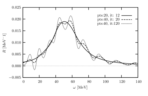
Figure 4: Fridman inversion results for the first test case (full: 20 grid-points and 12 iterations, dashed: 40 and 20, dotted: 40 and 120).

In fig. 4 we illustrate examplarily the procedure to determine the inversion for the Fridman case. First the number of iterations is fixed to 120 and the integration is done on a grid with 40 points (curve: pts:40, it:120). This curve shows still quite large unphysical oscillations although the integration grid consists of only 40 grid-points. By further reducing the amount of iterations to 20 (curve: pts:40, it: 20) the amplitude of the unphysical oscillations is reduced. Then we lower the amount of grid points till a smooth curve is obtained. At that point a strong regularization is introduced. To improve the threshold region the grid $(x_{i})$ is split up into two grids, a small inner grid using the simple integration method (eq. (18)) and an outer grid using a Gauss-Legendre integration grid. Finally a systematic variation of the number of grid points, grid boundaries and the number of iterations yields a parameter set where the result is stable under small changes of these parameters. The result shown fig. 4 and fig. 5 is obtained with 12 iteration where 6 points are used for the inner grid $[0,30]$ MeV and 14 points for the outer one $]30,197]$ MeV.

A similar pattern occurs also for the Banach method. Concerning the chosen resolution, we use here 24 Gaussian mesh points for the evaluation of the integrals and stop the iteration process for ${\cal E}_{l}<10^{-5}$. In contrast, if the Lorentzian is numerically better determined, like in our second example discussed below, typically a couple of hundreds of mesh points and termination conditions like ${\cal E}_{l}<10^{-15}$ (or even less) can be used for small $\sigma_{\rm I}$ without producing unphysical numerical oscillations in the resulting response $R$.

Our deuteron example has the great advantage that $R(\omega)$ can also be determined directly from eq. (2), since two-nucleon continuum wave functions can be calculated without problems. In fig. 5 we compare this response function, which is also taken from LIT , to those from the three inversion methods. It is evident that in spite of the strong regularization the inversion results lead to an overall correct description and form a kind of error band. The wavelet and Banach inversions oscillate around the true response with an error of less than 2 or 3 % in the peak region. The Fridman inversion exhibits a different pattern, but also describes the peak region quite well. The relative errors become somewhat larger at lower and higher energies. Nonetheless in comparison to the standard inversion method, which leads to very strong low-energy oscillations (see LIT ), our present results have a much smoother and more correct form at lower energies. It is important to note that errors of the inversion results are due to a not sufficiently precisely determined LIT. In fact as shown in ref. LIT the error of the LIT amounts up to 1.5 % in the peak region and up to about 4 % beyond 120 MeV. One sees that an error in the transform leads to an error of similar size in the inversion. Thus more precise results could be obtained by calculating the LIT with a higher precision. However, even with the present precision the low-energy shoulder could be described much better if one makes separate inversions for the C0 and C2 transition strength as was done in ref. LIT .

After our first example, which checked the proper implementation of the regularization into the various inversion methods, we turn to our high-precision test. In fig. 6 we show the chosen $R(\omega)$ up to $\omega=120$ MeV. The response function exhibits two peaks, one at $\omega=20$ MeV and the second at $\omega=50$ MeV. Both peaks have the same heights, but different widths. The corresponding LITs with $\sigma_{\rm I}=5$, 10, 20, and 40 MeV are illustrated in fig. 7. It is evident that only the smallest value of $\sigma_{\rm I}$ leads also to two peaks for the transform, while the information about the two separate peaks is more and more smeared out with increasing $\sigma_{\rm I}$.

In order to invert the LIT we calculate $L(\sigma_{\rm R},\sigma_{\rm I})$ for each of the four $\sigma_{\rm I}$ values from $\sigma_{\rm R}=-10$ MeV to $\sigma_{\rm R}=210$ MeV at 441 equidistant grid points. It is instructive to use the standard LIT inversion method, described in section IIIA, for the transform with the highest resolution ($\sigma_{\rm I}=5$ MeV). In fig. 8 it is shown that the result is not of a very high quality. There are low-energy oscillations and the two peaks are not well reproduced. One sees that the standard inversion method has difficulties to reproduce a more structured response function like our present double peak example. The reason for the problem are the basis functions. They have a too large extension in the $\omega$-space, therefore oscillations are introduced easily. In case of a more simpler structure like a single peak response such difficulties do not appear (see e.g. LIT ). We do not show results with the standard inversion method for larger values of $\sigma_{\rm I}$. As one may expect they lead to even worse results.

It is obvious that alternative inversion methods are needed in case of more structured response functions. In fact the three inversion techniques described in sections IIIB-D lead to much better results. For $\sigma_{\rm I}=5$ and 10 MeV one obtains results so close to the true $R$ that in fig. 6 they would all appear identical to the true response function. Thus in fig. 9 we show the relative errors of $R$ in an $\omega$-range, where $R(\omega)$ is not too close to 0. It is evident that the relative errors are very small: generally much less than 0.001 for $\sigma_{\rm I}=5$ MeV and less than 0.01 for $\sigma_{\rm I}=10$ MeV, only close to the low- and high-energy borders, where $R$ approaches 0 the error can become a bit larger. Here we would like to point out that the threshold region can also be inverted with greater care (see final paragraph of subsection IIIA). In figs. 10 and 11 we illustrate the inversion results for the two higher $\sigma_{\rm I}$ values. One sees that one still obtains rather good results with $\sigma_{\rm I}=20$ MeV, particularly with wavelet and Banach’s fix point theorem inversion techniques. With $\sigma_{\rm I}=40$ MeV the inversion results become worse. The shapes of the two peaks are not very well reproduced, but at least the peaks are recognized as two separate structures and also the high-energy tail is still rather well described. However, it is obvious that for the present case a $\sigma_{\rm I}$ value of 40 MeV is not sufficient to have precise inversion results. On the other hand with a further increase of the numerical precisions in calculating the transform and the inversions, which is nothing else than a further reduction of the regularization, one could have also for $\sigma_{\rm I}=40$ MeV much better results.

In the above example Fridman and Banach methods lead to a single inversion result for a given $\sigma_{\rm I}$, while the wavelet technique leads for any set of values for $M$ and $N_{m}$ (see table I) to principally different inversion results, in absence of unphysical oscillations they are of course almost identical. For $\sigma_{\rm I}=5$, 10, and 20 MeV the result with the best description of $L(\sigma_{\rm R},\sigma_{\rm I})$ (sum of quadratic errors) is taken ($\sigma_{\rm I}=5$ and 10 MeV: $M=2$ and $N_{0}=N_{1}=N_{2}=63$, $\sigma_{\rm I}=20$ MeV: $M=2$ and $N_{0}=63$, $N_{1}=31$, $N_{2}=15$). For $\sigma_{\rm I}=40$ MeV, however, the inversion result with the smallest error shows strong and unrealistic oscillations (see fig. 12) and is thus discarded. Also the 14 next best fits lead to similar unrealistic oscillations showing that also for this case a rather strong regularization is necessary. Only the 16th best result ($M=0$, $N_{0}=63$) does not exhibit such an unrealistic pattern and is therefore shown in fig. 11. Such strongly oscillating solutions like that of fig. 12 can be identified easily as unrealistic, since a true response function has to be positive definite and in addition it is difficult to imagine that a true response can exhibit such a regular oscillation pattern.

We summarize our results as follows. The various newly introduced inversion techniques for the Lorentz Integral Transform contain a proper regularization method and are thus able to treat the ill-posed inversion problem. In addition all these techniques are capable to invert also transforms of responses with rather complicated structures with a very high precision. For such cases they lead to considerably better inversion results than the standard LIT inversion method. Our results show that the LIT approach is not restricted to treat cases, where simple structures appear, but is suitable for many different applications.

Appendix A Mathematical proofs concerning the fixpoint method

A.1 Proof of (31)

In order to prove (31), let’s consider the expression

$$B(\omega,\sigma_{\rm I}):=\Im\int d\omega^{\prime}\frac{R(\omega^{\prime})}{\omega^{\prime}-\omega-i\sigma_{\rm I}}\,\,,$$ (38)

which can be rewritten in two different manners: First, one has the identity

$$B(\omega,\sigma_{\rm I})=\Im\int d\omega^{\prime}\frac{R(\omega^{\prime})(\omega^{\prime}-\omega+i\sigma_{\rm I})}{(\omega^{\prime}-\omega)^{2}+\sigma_{\rm I}^{2}}=\sigma_{\rm I}L(\omega,\sigma_{\rm I})$$ (39)

and second, one can write

$$B(\omega,\sigma_{\rm I})=\Im\int d\omega^{\prime}\frac{R(\omega^{\prime})-R(\omega)}{\omega^{\prime}-\omega-i\sigma_{\rm I}}+\Im\left(R(\omega)\int d\omega^{\prime}\frac{1}{\omega^{\prime}-\omega-i\sigma_{\rm I}}\right)\,.$$ (40)

The second integral on the right hand part of (40) can be easily solved with the help of

$$\frac{a}{\pi}\int_{-\infty}^{\infty}dx\frac{1}{x^{2}+a^{2}}=1\,\,,\quad\quad(a>0)\,\,.$$ (41)

Comparison of (40) and (39) yields then (31).

A.2 Proof of uniqueness of iteration procedure

In this appendix we prove that there exists an $\epsilon>0$ so that for all $\sigma_{\rm I}<\epsilon$ the series (32) converges uniquely against a function $R^{\rm fix}$ which is identical with the desired response $R(\omega)$.

For that purpose, let us introduce the difference

$$\Delta^{(n)}:=R-R^{(n)}\,.$$ (42)

Exploiting (30),(31),(32), the function $\Delta$ fulfills

$$\Delta^{(n+1)}:={\cal T}\Delta^{(n)}$$ (43)

with the linear mapping

$${\cal T}\Delta^{(n)}(\omega)=-\frac{\sigma_{\rm I}}{\pi}\int d\omega^{\prime}\frac{\Delta^{(n)}(\omega^{\prime})-\Delta^{(n)}(\omega)}{(\omega^{\prime}-\omega)^{2}+\sigma^{2}_{\rm I}}\,.$$ (44)

At next, we will prove that $\cal{T}$ is – for sufficiently small $\sigma_{\rm I}$ – a contractive linear mapping, i.e. there exists a constant $0<q<1$ so that

$$||{\cal T}\Delta^{(n)}||^{2}\equiv||\Delta^{(n+1)}||^{2}\leq q||\Delta^{(n)}||^{2}\,\,.$$ (45)

Proof:

For the norm of $\Delta^{(n+1)}$ we obtain

$$||\Delta^{(n+1)}||^{2} = \int d\omega\Delta^{(n+1)}(\omega)\Delta^{(n+1)}(\omega)$$ (46)

$$\!\!\!\!\!\!\!\!\!\!\!\!\!\!\!\!\!\!\!\!\!\!\!\!\!\!\!\!\!\!\!\!\!\!\!\!\!\!\!\!\!\!\!\!\!\!\!\!\!\!\!\!\!\!\!\!\!\!=\frac{\sigma_{\rm I}^{2}}{\pi^{2}}\int d\omega\int d\omega^{\prime}\int d\omega^{\prime\prime}\left(\frac{\Delta^{(n)}(\omega^{\prime})-\Delta^{(n)}(\omega)}{(\omega^{\prime}-\omega)^{2}+\sigma_{\rm I}^{2}}\right)\left(\frac{\Delta^{(n)}(\omega^{\prime\prime})-\Delta^{(n)}(\omega)}{(\omega^{\prime\prime}-\omega)^{2}+\sigma_{\rm I}^{2}}\right)\,\,,$$

which can be rewritten as

$$||\Delta^{(n+1)}||^{2} = \frac{\sigma_{\rm I}^{2}}{\pi^{2}}\int d\omega\int d\omega^{\prime}\int d\omega^{\prime\prime}\left(\frac{1}{(\omega^{\prime}-\omega)^{2}+\sigma_{\rm I}^{2}}\,\,\right)\,\,\left(\frac{1}{(\omega^{\prime\prime}-\omega)^{2}+\sigma_{\rm I}^{2}}\right)$$

$$\!\!\!\!\!\!\!\!\!\!\!\!\!\!\!\!\!\!\!\!\!\!\!\!\!\!\!\!\!\!\!\!\!\!\!\!\!\!\!\!\!\!\!\!\!\!\left(\Delta^{(n)}(\omega^{\prime})\Delta^{(n)}(\omega^{\prime\prime})+\Delta^{(n)}(\omega)\Delta^{(n)}(\omega)-\Delta^{(n)}(\omega^{\prime})\Delta^{(n)}(\omega)-\Delta^{(n)}(\omega^{\prime\prime})\Delta^{(n)}(\omega)\right)\,\,.$$

This expression can be simplified with the help of (41) and with the identity (which can be easily proven using the method of residues)

$$\int_{-\infty}^{\infty}d\omega\left(\frac{1}{(\omega^{\prime}-\omega)^{2}+\sigma_{\rm I}^{2}}\,\,\right)\,\,\left(\frac{1}{(\omega^{\prime\prime}-\omega)^{2}+\sigma_{\rm I}^{2}}\right)=\frac{2\pi}{\sigma_{\rm I}}\left(\frac{1}{(\omega^{\prime}-\omega^{\prime\prime})^{2}+4\,\sigma_{\rm I}^{2}}\,\,\right)$$ (48)

as follows:

$$||\Delta^{(n+1)}||^{2}=||\Delta^{(n)}||^{2}+\frac{2\sigma_{\rm I}}{\pi}\mbox{$\langle\Delta^{(n)}|$}{\widehat{L}}(2\sigma_{\rm I})\mbox{$|\Delta^{(n)}\rangle$}-\frac{2\sigma_{\rm I}}{\pi}\mbox{$\langle\Delta^{(n)}|$}{\widehat{L}}(\sigma_{\rm I})\mbox{$|\Delta^{(n)}\rangle$}\,\,.$$ (49)

For further exploitation, let’s prove at next the following

Lemma: There exists an $\epsilon>0$, so that for all $\sigma_{\rm I}<\epsilon$

$$\frac{2\sigma_{\rm I}}{\pi}\mbox{$\langle\Delta^{(n)}|$}{\widehat{L}}(2\sigma_{\rm I})\mbox{$|\Delta^{(n)}\rangle$}\leq A(\sigma_{\rm I})\mbox{$\langle\Delta^{(n)}|\Delta^{(n)}\rangle$},$$ (50)

where the upper limit $A(\sigma_{\rm I})$ for $\sigma_{\rm I}<\epsilon$ fulfills the estimate

$$1-\delta\leq A\leq 1+\delta,\quad\quad\delta<\frac{1}{3}\,\,.$$ (51)

Proof of the Lemma:

Due to

$$\lim_{\sigma_{\rm I}\rightarrow\infty}\frac{\sigma_{\rm I}}{\pi}\frac{1}{(x-y)^{2}+\sigma_{\rm I}^{2}}=\delta(x-y)\,\,,$$ (52)

the statement is obviously true for $\sigma_{\rm I}\rightarrow 0$ with

$$\lim_{\sigma_{\rm I}\rightarrow 0}A(\sigma_{\rm I})=1\,\,.$$ (53)

Because the LIT-operator in (29) is depending analytically on the parameter $\sigma_{\rm I}$, the statement follows immediately.

With the help of the Lemma, one obtains for (49) the following estimate:

$$||\Delta^{(n+1)}||^{2} = |||\Delta^{(n)}||^{2}+\frac{2\sigma_{\rm I}}{\pi}\mbox{$\langle\Delta^{(n)}|$}{\widehat{L}}(2\sigma_{\rm I})\mbox{$|\Delta^{(n)}\rangle$}-\frac{2\sigma_{\rm I}}{\pi}\mbox{$\langle\Delta^{(n)}|$}{\widehat{L}}(\sigma_{\rm I})\mbox{$|\Delta^{(n)}\rangle$}|$$ (54)

$$\leq |1+(1+\delta)-2(1-\delta)|\quad||\Delta^{(n)}||^{2}$$

$$= 3\delta||\Delta^{(n)}||^{2}\,\,.$$

Due to

$$q:=3\delta<3\frac{1}{3}=1\,\,,$$ (55)

the mapping $\Delta^{(n)}\rightarrow\Delta^{(n+1)}$ defined via (43) is therefore for $\sigma_{\rm I}<\epsilon$ contracting.

In consequence, we can now apply Banach’s Fixpoint Theorem: It states that the series $\Delta^{(n)}$ converges uniquely against a fixpoint $\Delta$. Obviously, (43) is fulfilled by $\Delta^{(n)}=0$ for all $n$, so that therefore

$$\Delta^{(n)}\rightarrow\Delta=0\,\,$$ (56)

and therefore, due to (42), $R^{(n)}\rightarrow R$ uniquely.

A.3 Incorporation of correct threshold behaviour of the response function

If the lower and upper value of the integral (29) are not any longer $\pm\infty$, but some finite values $a$ and $b$, the proofs presented in appendix A.1 and A.2 have to be solely repeated where instead of the expression (41) its counterpart for finite integrals

$$\frac{a}{\alpha_{(a,b)}(\omega)}\int_{a}^{b}dx\frac{1}{x^{2}+a^{2}}=1\quad\quad(a>0)$$ (57)

has to be used (the function $\alpha$ is given in (36)). Therefore, instead of (31) one has the identity

$$R(\omega) = \frac{\sigma_{\rm I}}{\alpha_{(a,b)}(\omega)}L(\omega,\sigma_{\rm I})-\frac{\sigma_{\rm I}}{\alpha_{(a,b)}(\omega)}\int_{a}^{b}d\omega^{\prime}\frac{R(\omega^{\prime})-R(\omega)}{(\omega^{\prime}-\omega)^{2}+\sigma^{2}_{\rm I}}\,\,,$$ (58)

which motivates therefore the mapping ${\hat{T}}_{(a,b)}(\sigma_{\rm I},L)$ according to (35).

The counterpart of the difference function (42) now becomes

$$\Delta_{(a,b)}^{(n+1)}(\omega):=R-R^{(n)}_{(a,b)}=-\frac{\sigma_{\rm I}}{\alpha_{(a,b)}(\omega)}\int_{a}^{b}d\omega^{\prime}\frac{\Delta_{(a,b)}^{(n)}(\omega^{\prime})-\Delta_{(a,b)}^{(n)}(\omega)}{(\omega^{\prime}-\omega)^{2}+\sigma^{2}_{\rm I}}\,\,.$$ (59)

The norm of this function

$$||\Delta_{(a,b)}^{(n+1)}||^{2}=\int_{a}^{b}d\omega\Delta_{(a,b)}^{(n+1)}(\omega)\Delta_{(a,b)}^{(n+1)}(\omega)$$

$$=\int_{a}^{b}d\omega\int_{a}^{b}d\omega^{\prime}\int_{a}^{b}d\omega^{\prime\prime}\left(\frac{\sigma_{\rm I}}{\alpha_{(a,b)}(\omega)}\right)^{2}\left(\frac{1}{(\omega^{\prime}-\omega)^{2}+\sigma_{\rm I}^{2}}\,\,\right)\,\,\left(\frac{1}{(\omega^{\prime\prime}-\omega)^{2}+\sigma_{\rm I}^{2}}\right)$$

$$\left(\Delta_{(a,b)}^{(n)}(\omega^{\prime})\Delta_{(a,b)}^{(n)}(\omega^{\prime\prime})+\Delta_{(a,b)}^{(n)}(\omega)\Delta_{(a,b)}^{(n)}(\omega)-\Delta_{(a,b)}^{(n)}(\omega^{\prime})\Delta_{(a,b)}^{(n)}(\omega)-\right.$$

$$\left.\Delta_{(a,b)}^{(n)}(\omega^{\prime\prime})\Delta_{(a,b)}^{(n)}(\omega)\right)\,\,.$$ (60)

is much more complicated to be handled than its counterpart (LABEL:bew6a): Due to the finite limits in the integrals, the method of residues cannot any longer be used. Moreover, the constant factor $\pi$ in (LABEL:bew6a) now turns into the complicated function $\alpha_{(a,b)}(\omega)$ so that a simple relation like (49) is not any longer valid. However, recalling the representation (52) of the $\delta$-function as well as (for arbitrary $a,b$; provided $a<\omega<b$)

$$\lim_{\sigma_{\rm I}\rightarrow 0}\alpha_{(a,b)}(\omega)=\pi\,\,,$$ (61)

it is obvious that for sufficiently small $\sigma_{\rm I}$ the influence of the finite limits $a$ and $b$ in the integrals dies out so that again the mapping $\Delta_{(a,b)}^{(n)}\rightarrow\Delta_{(a,b)}^{(n+1)}$ is a contractive one.

Figure 1: Mexican hat wavelet (eq. (10)).

Figure 2: LIT of the first test case taken from LIT

Figure 3: Wavelet inversion results for the first test case with $M=0$ (full: $N_{0}=15$, dashed: $N_{0}=31$).

Figure 5: Final inversion results with the three new methods for the first test case are shown (upper panel; full: original response function, dashed: wavelet, dashed-dotted: Fridman, dotted: Banach) along with their relative error (lower panel).

Figure 6: Double peaked response function of second test case.

Figure 7: LIT of the double peaked response function with different $\sigma_{\rm I}$ (curves for $\sigma_{\rm I}=10$, 20 and 40 MeV are scaled by factors of 2, 4 and 8, respectively).

Figure 8: Result for $\sigma_{\rm I}=5$ MeV (dashed) obtained with the standard method (sec. IIIA) for the second test case and the original double peaked response function (full).

Figure 9: Relative error of the inversion results for the second test case obtained with the new methods (full: wavelet, crosses: Fridman, points: Banach) for $\sigma_{\rm I}=5$ MeV (upper panel) and for $\sigma_{\rm I}=10$ MeV (lower panel).

Figure 10: Results of the three new inversion methods (full: original response function, dashed: wavelet, dashed-dotted: Fridman, dotted: Banach) for the second test case with $\sigma_{\rm I}=20$ MeV are shown (upper panel) along with their relative error (lower panel; full: wavelet, crosses: Fridman scaled by a factor of $0.2$, points: Banach).

Figure 11: Results of the three new inversion methods (full: original response function, dashed: wavelet, dashed-dotted: Fridman, dotted: Banach) for the second test case with $\sigma_{\rm I}=40$ MeV are shown (upper panel) along with their relative error (lower panel).

Figure 12: Wavelet inversion results for second test case (full: $M=0$, $N_{0}=31$, dashed: $M=2$, $N_{2}=31$, $N_{1}=15$, $N_{2}=7$).

References

- (1) V. Efros, W. Leidemann, G. Orlandini, Phys. Lett. B 338, 130 (1994).
- (2) V. Efros, W. Leidemann, G. Orlandini, Phys. Rev. Lett. 78, 432 (1997).
- (3) V.D. Efros, W. Leidemann, G. Orlandini, E.L. Tomusiak, Phys. Rev. C 69, 044001 (2004).
- (4) V. Efros, W. Leidemann, G. Orlandini, Phys. Rev. Lett. 78, 4015 (1997).
- (5) S. Bacca, M. Marchisio, N. Barnea, W. Leidemann, G. Orlandini, Phys. Rev Lett. 89, 052502 (2002).
- (6) S. Bacca, H. Arenhövel, N. Barnea, W. Leidemann, G. Orlandini, Phys. Lett. B 603.
- (7) A. La Piana, W. Leidemann, Nucl. Phys. A 677, 423 (2000).
- (8) S. Quaglioni, N. Barnea, V.D. Efros, W. Leidemann, G. Orlandini, Phys. Rev. C 69, 044002 (2004).
- (9) C. Reiß, E.L. Tomusiak, W. Leidemann, G. Orlandini, Eur. Phys. J. A 17, 589 (2003).
- (10) D. Gazit, N. Barnea, Phys. Rev. C 70, 048801 (2004).
- (11) V. Efros, W. Leidemann, G. Orlandini, Few-Body Syst. 26, 251 (1999).
- (12) H. Kamada et al., Phys. Rev. C 64, 044001 (2001).
- (13) D. Andreasi, thesis, Università di Trento (2005).
- (14) V. M. Fridman, Uspekhy Mat. Nauk 11, 233 (1956).