Semileptonic Decays of Heavy Lambda Baryons in a Quark Model

Abstract

JLAB-THY-05-304

I Introduction and Motivation

Many of the parameters of the Standard Model (SM), including the Cabbibo-Kobayashi-Maskawa (CKM) CKM matrix elements, are not yet determined with ‘satisfactory’ precision. Very precise knowledge of these matrix elements is important as they play a crucial role in the search for answers to some fundamental questions, such as the nature of $CP$ violation and the unitarity of the CKM matrix. Semileptonic decays of hadrons have been, and will continue to be, the main source of information on the CKM matrix elements. The precision with which the CKM matrix elements are extracted from these semileptonic decays is strongly dependent on how well the form factors that describe the matrix elements of the hadronic currents are known. The vast literature on these form factors is a testament to the importance of these parameters.

The semileptonic decays of heavy mesons have been studied extensively in the last two decades. Wirbel, Stech and Bauer WSB ; BW assumed monopole type form factors for the decays of heavy mesons. In Ref. ISGW ; ISGW1 , a non-relativistic quark model (NRQM) was used to treat the semileptonic decays of $B$ and $D$ mesons, and relatively simple forms for the form factors were presented. The first of those articles, along with the work of Shifman and Voloshin voloshin , ultimately lead to the development of the heavy quark effective theory (HQET). In addition, Ivanov and Santorelli ISA used a relativistic quark model to find the form factors. These are just a very few of the very large number of articles that treat semileptonic decays of mesons in some kind of model.

Weak decays of hadrons involving one or more heavy quarks $(m_{Q}>>\Lambda_{QCD})$ have an additional symmetry in the effective Lagrangian which was first pointed out by Isgur and Wise IW . There, they used the additional heavy quark symmetry to obtain normalized, model-independent predictions for all the form factors for the decays of heavy hadrons to daughter hadrons that are also heavy. This led to many subsequent calculations by many authors.

For the hadronic matrix elements of the electroweak currents between two heavy mesons, the application of HQET provides a number of features that simplify the extraction of CKM matrix elements from such decays. First, the number of form factors is reduced, so that the six form factors that describe the decays of heavy pseudoscalar mesons to heavy pseudoscalar and vector mesons are replaced by a single form factor, at leading order in HQET. This form factor has become known as the Isgur-Wise function. Second, the absolute normalization of this form factor at the so-called non-recoil point is known. Third, corrections to this normalization do not arise at order $1/m_{Q}$ in the heavy quark expansion, but at order $1/m_{Q}^{2}$. This is known as Luke’s Theorem luke , and is an analog of the Ademollo-Gatto theorem gatto . This means that some predictions made at leading order are more robust than might be expected. Finally, the corrections that do arise can be estimated systematically in the heavy quark expansion. As a result, HQET has become the tool of choice in the extraction of $|V_{cb}|$ pdg .

For the semileptonic decays of a heavy meson to a light meson, the predictions of HQET are not quite as powerful: there is no reduction in the number of form factors needed to describe the decay, nor are the normalizations of any of the form factors known. However, the heavy quark symmetry, along with SU(2) or SU(3) flavor symmetry for the light mesons, can be used to relate the form factors for $D\to\pi$ and $D\to\rho$ decays, for instance, to those for $B\to\pi$ and $B\to\rho$ decays, respectively. Thus, even though it is not as predictive in the decays of heavy to light mesons, there is still a great deal of reliance on HQET for extracting $V_{ub}$ from meson decays.

For the semileptonic decays of a heavy baryon to another heavy baryon, HQET makes predictions that are completely analogous to those made for heavy-to-heavy meson decays: (i) the six form factors that describe the decays to the ground-state heavy baryons are replaced by a single form factor, the Isgur-Wise function; (ii) the normalization of the Isgur-Wise function is known at the non-recoil point; (iii) corrections to this normalization first appear at order $1/m_{Q}^{2}$; (iv) corrections can be systematically estimated in a $1/m_{Q}$ expansion.

In the case of a heavy baryon decaying to a light baryon, HQET makes predictions that are not as powerful as in the heavy-to-heavy case, but which are significantly more powerful than for the heavy-to-light transitions of mesons. Among the baryons, the leading-order prediction is that the number of independent form factors decreases from six to two. In addition, as with mesons, the heavy quark symmetry can be used to relate the form factors for the decay $\Lambda_{c}^{+}\to n$ to those for $\Lambda_{b}\to p$, for instance. This, in principle, could facilitate the extraction of $V_{ub}$ from semileptonic decays of the $\Lambda_{b}$, and since the number of unknown form factors is reduced from six to two, the theoretical uncertainty in the extraction from these decays should be significantly smaller than extractions from meson decays.

While HQET has been tremendously successful and useful in treating semileptonic decays of heavy hadrons, it is not without its limitations. It is a limit of QCD that applies only to hadrons containing heavy quarks. For the decays of such hadrons, it only predicts the relationships among form factors, not their kinematic dependence; ansätze, models of one kind or another, or lattice simulations, are still needed for this. In addition, the predictions of HQET are valid only as long as the energy of the daughter hadron is not comparable to the mass of the heavy quark. For heavy to heavy decays, this means that the predictions are valid for all of the available phase space, but for heavy to light decays, such as $B\to\pi$, a large portion of the available phase space is beyond the region of reliable applicability of HQET. These limitations mean that the predictions of HQET must be complemented/supplemented by information arising from other approaches to hadron structure.

While some work has been done in modeling the form factors for the semileptonic decays of heavy baryons, to the best of our knowledge little has been done in treating the decays to excited baryons. Predictions for the number of independent form factors for decays to excited states have been made in the framework of HQET robertsa , and Leibovich and Stewart LS have examined the form factors for decays to the $1/2^{-}$ and $3/2^{-}$ states, using large $N_{c}$ arguments. In the semileptonic decays of $B$ mesons to those with charm, it is known that $B^{0}$ decays to the ground state pseudoscalar and vector mesons provide only about 75% of the total semileptonic decay rate, while for the $B^{\pm}$, the corresponding fraction is about 85%. Any assumption that decay of a heavy baryon to the ground state will saturate the semileptonic decay rate is therefore subject to potentially large corrections.

In some of the work done in this area, the predictions of HQET, along with various ansätze for the form factors, have been used to estimate some decay rates. Leibovich and Stewart LS follow such a procedure to estimate the rates for decays of the $\Lambda_{b}$ to the $J^{P}=1/2^{-}$ and $3/2^{-}$ $\Lambda_{c}$ states. Polarization effects in semileptonic $\Lambda_{b}$ and $\Lambda_{c}$ decays have been studied by Körner and Krämer KK , using the predictions of HQET to estimate the dominant form factors for both $b\to c$ and $c\to s$ transitions. They have also calculated the asymmetry parameters that characterize the angular dependence of the decay distributions.

A number of authors have constructed explicit quark models of the form factors for the decays of $\Lambda_{Q}$ baryons to ground state baryons. The decays of $\Lambda_{b}$ and $\Omega_{b}$ have been treated by Singleton using a spectator quark model SING . He also discusses the polarization of the $W$ boson and the daughter baryon in these processes. Albertus et al. Albertus use a NRQM to evaluate the form factors for $\Lambda_{b}\to\Lambda_{c}$, explicitly applying heavy quark symmetry to their trial wave functions. To date, there appear to be only two lattice studies of the semileptonic decays of heavy baryons. A first study of $\Lambda_{b}$ and $\Xi_{b}$ semileptonic decays was made by Bowler et al. Richards , while Gottlieb and Tamhankar gottlieb have examined the decay of the $\Lambda_{b}$. Pérez-Marcial and collaborators huerta have studied the semileptonic decays of a number of charmed baryons, both in a non-relativistic quark model and in the MIT bag model. There have been light-front calculations lightfront , as well as ones using sum rules sum , Bethe-Salpeter formalisms BSF , bag models bag , and quark model calculations qmc . Large $N_{c}$ arguments have also been applied to these form factors largen , as well as perturbative QCD arguments pqcd . For the decays of a heavy baryon to a light one, work has been done using QCD sum rules sumlight , and there’s one quark model calculation qmclight apart from the work of Scora scora , to the best of our knowledge.

The experimental status of heavy baryon semileptonic decays is somewhat rudimentary. The semileptonic decay rate for $\Lambda_{c}\to\Lambda$ has been measured by the CLEO and Argus collaborations argus ; CLEO , while the Delphi collaboration has only recently published an analysis of the exclusive semileptonic decay of the $\Lambda_{b}$ delphi . Prior to this, only the inclusive semileptonic branching fraction $\Lambda_{b}\to\Lambda_{c}\ell\nu X$ had been reported in the PDG pdg . In their analysis of the $\Lambda_{c}\to\Lambda$ semileptonic decay, the CLEO collaboration have assumed that the ground state $\Lambda$ saturates the semileptonic decays of the $\Lambda_{c}$, and cite the absence of any final states of the form $\Lambda\ell\nu$ with additional decay products from the $\Lambda_{c}$ to support their assumption CLEO . No experiments have yet reported results for the decay $\Lambda_{c}\to n$.

The major difficulty in the baryon sector is that there is no source of heavy baryons as there is for mesons. Electron-positron colliders have produced billions of $B$ mesons, utilizing the fact that the $\Upsilon(4s)$ is just above the $B\overline{B}$ threshold. In principle, a similar abundance can be duplicated among $D$ mesons, by using the $\Psi(3s)$. With baryons, production at such machines will be continuum production, as there are no (known) resonances to enhance the rate of production. Hadron colliders can provide larger yields, but they provide large yields of everything, and the heavy baryons will then have to be separated from everything else that is produced. However, the recent CLEO measurement suggests that some optimism regarding the future measurement of these decays might be warranted. In addition, there might be prospects for such studies at Jefferson Laboratory upgraded to 12 GeV or higher, or at E907 at FNAL. The advantage in these cases is that the target will be a baryon, unlike the continuum production of $e^{+}e^{-}$ machines.

In this paper we study the semileptonic decay of $\Lambda_{Q}$ baryons, the motivation for which is two-fold. One of our motivations is the importance of the CKM matrix elements $V_{ub}$ and $V_{cb}$, and that baryon semileptonic decays can provide complementary extractions of these quantities, despite the difficulties mentioned above. In particular, a model such as ours, coupled with constraints provided by HQET, may lead to a more precise extraction of $V_{ub}$ than provided by meson decays.

Our second motivation is to examine the predictions for these decays of a quark model developed very much in the spirit of the work by Capstick and Isgur CI , which builds on the work of Isgur and Karl IsgurKarl- ; IsgurKarl . Such a model has been applied, with some success, to the strong capstickroberts and electromagnetic capstickkeister ; Capstick couplings of baryons, and the semileptonic decays of baryons is a useful complementary extension of such a model. Indeed, a similar model, applied to the semileptonic decays of mesons ISGW , gave rise to HQET. We note that the thesis of Scora scora treats a number of baryon semileptonic decays in a framework very similar to that used in the treatment of mesons in ISGW . We use a similar framework, but we extend the model to examine the decays to excited baryons, whereas Scora scora examined only decays to ground state baryons. We also use a more sophisticated treatment of baryon structure.

This manuscript is organized as follows: in Section II we discuss the hadronic matrix elements and decay rates. Section III presents a brief outline of heavy quark effective theory as it relates to the decays that we discuss. In Section IV we describe the model we use to obtain the form factors, including some description of the Hamiltonian. Our analytic results are discussed in Section V, our numerical results are given in section VI, and Section VII presents our conclusions and outlook. A number of details of the calculation, including the explicit expressions for the form factors, are shown in a number of Appendices.

II Matrix Elements and Decay Rates

II.1 Matrix Elements

The transition matrix element for semileptonic decay of $\Lambda_{Q}$ $(\Lambda_{Q}\rightarrow\Lambda_{q}\ell\nu_{\ell})$ is

$$T=\frac{G_{F}}{\sqrt{2}}V_{Qq}\overline{u_{\ell}}\gamma^{\mu}(1-\gamma_{5})u_{\nu_{\ell}}\langle\Lambda_{q}(p^{\prime},s^{\prime})|J_{\mu}|\Lambda_{Q}(p,s)\rangle,$$ (1)

where $G_{F}/\sqrt{2}=g^{2}/(8M_{W}^{2})$ is the Fermi coupling constant, $M_{W}$ is the intermediate vector boson mass, $V_{Qq}$ is the CKM matrix element, and $\overline{u_{\ell}}\gamma^{\mu}(1-\gamma_{5})u_{\nu_{\ell}}$ is the lepton current. Since quarks are confined, the matrix element of the hadron current is described in terms of a number of form factors. We will build a model of the baryons we wish to study, and obtain approximations to the form factors that describe the hadronic matrix elements. For transitions between ground state $(J^{P}=1/2^{+})$ baryons, the hadronic matrix elements of the vector and axial currents are

$$\langle\Lambda_{q}(p^{\prime},s^{\prime})|V_{\mu}|\Lambda_{Q}(p,s)\rangle = \overline{u}(p^{\prime},s^{\prime})\left(F_{1}(q^{2})\gamma_{\mu}+F_{2}(q^{2})\frac{p_{\mu}}{m_{\Lambda_{Q}}}+F_{3}(q^{2})\frac{p^{\prime}_{\mu}}{m_{\Lambda_{q}}}\right)u(p,s),$$ (2)

$$\langle\Lambda_{q}(p^{\prime},s^{\prime})|A_{\mu}|\Lambda_{Q}(p,s)\rangle = \overline{u}(p^{\prime},s^{\prime})\left(G_{1}(q^{2})\gamma_{\mu}+G_{2}(q^{2})\frac{p_{\mu}}{m_{\Lambda_{Q}}}+G_{3}(q^{2})\frac{p^{\prime}_{\mu}}{m_{\Lambda_{q}}}\right)\gamma_{5}u(p,s),$$ (3)

where the $F_{i}$ and $G_{i}$’s are baryon form factors which depend on the square of the momentum transfer $q=p-p^{\prime}$ between the initial and the final baryons. Similarly, the matrix elements for decays to a daughter baryon with $J^{P}=3/2^{-}$ are

$$\langle\Lambda_{q}^{3/2}(p^{\prime},s^{\prime})|V_{\mu}|\Lambda_{Q}(p,s)\rangle = \overline{u}^{\alpha}(p^{\prime},s^{\prime})\left[\frac{p_{\alpha}}{m_{\Lambda_{Q}}}\left(F_{1}\gamma_{\mu}+F_{2}\frac{p_{\mu}}{m_{\Lambda_{Q}}}+F_{3}\frac{p^{\prime}_{\mu}}{m_{\Lambda_{q}^{3/2}}}\right)+F_{4}g_{\alpha\mu}\right]u(p,s),$$

$$\langle\Lambda_{q}^{3/2}(p^{\prime},s^{\prime})|A_{\mu}|\Lambda_{Q}(p,s)\rangle = \overline{u}^{\alpha}(p^{\prime},s^{\prime})\left[\frac{p_{\alpha}}{m_{\Lambda_{Q}}}\left(G_{1}\gamma_{\mu}+G_{2}\frac{p_{\mu}}{m_{\Lambda_{Q}}}+G_{3}\frac{p^{\prime}_{\mu}}{m_{\Lambda_{q}^{3/2}}}\right)+G_{4}g_{\alpha\mu}\right]\gamma_{5}u(p,s).$$ (4)

The spinor $\overline{u}^{\alpha}(p^{\prime},s^{\prime})$ satisfies the conditions

$$p^{\prime}_{\alpha}\overline{u}^{\alpha}(p^{\prime},s^{\prime})=0,\,\,\,\,\overline{u}^{\alpha}(p^{\prime},s^{\prime})\gamma_{\alpha}=0,\,\,\,\,\overline{u}^{\alpha}(p^{\prime},s^{\prime})p\hskip-5.0pt/^{\prime}=m_{\Lambda_{q}^{3/2}}\overline{u}^{\alpha}(p^{\prime},s^{\prime}).$$ (5)

The corresponding matrix elements for decay to a baryon with $J^{P}=5/2^{+}$ are

$$\langle\Lambda_{q}^{5/2}(p^{\prime},s^{\prime})|V_{\mu}|\Lambda_{Q}(p,s)\rangle = \overline{u}^{\alpha\beta}(p^{\prime},s^{\prime})\frac{p_{\alpha}}{m_{\Lambda_{Q}}}\left[\frac{p_{\beta}}{m_{\Lambda_{Q}}}\left(F_{1}\gamma_{\mu}+F_{2}\frac{p_{\mu}}{m_{\Lambda_{Q}}}+F_{3}\frac{p^{\prime}_{\mu}}{m_{\Lambda_{q}^{5/2}}}\right)+F_{4}g_{\beta\mu}\right]u(p,s),$$

$$\langle\Lambda_{q}^{5/2}(p^{\prime},s^{\prime})|A_{\mu}|\Lambda_{Q}(p,s)\rangle = \overline{u}^{\alpha\beta}(p^{\prime},s^{\prime})\frac{p_{\alpha}}{m_{\Lambda_{Q}}}\left[\frac{p_{\beta}}{m_{\Lambda_{Q}}}\left(G_{1}\gamma_{\mu}+G_{2}\frac{p_{\mu}}{m_{\Lambda_{Q}}}+G_{3}\frac{p^{\prime}_{\mu}}{m_{\Lambda_{q}^{5/2}}}\right)+G_{4}g_{\beta\mu}\right]\gamma_{5}u(p,s),$$ (6)

where the spinor $\overline{u}^{\alpha\beta}(p^{\prime},s^{\prime})$ is symmetric in the indices $\alpha$ and $\beta$, and satisfies

$$p^{\prime}_{\alpha}\overline{u}^{\alpha\beta}(p^{\prime},s^{\prime}) = p^{\prime}_{\beta}\overline{u}^{\alpha\beta}(p^{\prime},s^{\prime})=0,$$

$$\overline{u}^{\alpha\beta}(p^{\prime},s^{\prime})\gamma_{\alpha} = \overline{u}^{\alpha\beta}(p^{\prime},s^{\prime})\gamma_{\beta}=0,$$

$$\overline{u}^{\alpha\beta}(p^{\prime},s^{\prime})p\hskip-5.0pt/^{\prime} = m_{\Lambda_{q}^{5/2}}\overline{u}^{\alpha\beta}(p^{\prime},s^{\prime}),$$

$$\overline{u}^{\alpha\beta}(p^{\prime},s^{\prime})g_{\alpha\beta} = 0.$$ (7)

Here we have only presented the form factor equations involving spinors having natural parity. The equations for unnatural parity spinors can be constructed in a similar manner by switching $\gamma_{5}$ from the equations defining the $G_{i}$ to the equations defining the $F_{i}$.

II.2 Decay Rates

The decay rate that arises from any of these matrix elements is

$$d\Gamma=\frac{1}{2m_{\Lambda_{Q}}}\frac{G_{F}^{2}}{2}|{V_{Qq}}|^{2}\left(\prod_{f}\frac{d^{3}p_{f}}{(2\pi)^{3}2E_{f}}\right)L^{\mu\nu}H_{\mu\nu}(2\pi)^{4}\delta^{(4)}(p_{A}-\sum{p_{f}}),$$ (8)

where $A$ refers to the initial hadron. The leptonic tensor $L^{\mu\nu}$ is

$$L^{\mu\nu}=8[p_{\ell}^{\mu}p_{\nu_{\ell}}^{\nu}+p_{\nu_{\ell}}^{\mu}p_{\ell}^{\nu}-g^{\mu\nu}p_{\ell}\cdot p_{\nu_{\ell}}+i\epsilon^{\mu\nu\alpha\beta}p_{\ell\alpha}p_{\nu_{\ell}\beta}].$$ (9)

The hadronic tensor $H_{\mu\nu}$ is

$$H_{\mu\nu}=\sum_{{\rm spin}}\langle\Lambda_{Q}|{J_{\nu}^{\dagger}}|\Lambda_{q}\rangle\langle\Lambda_{q}|J_{\mu}|\Lambda_{Q}\rangle,$$ (10)

where $\Lambda_{Q}$ and $\Lambda_{q}$ refer to the initial and final baryons, respectively. The tensor $H_{\mu\nu}$ must have the Lorentz structure

$$H_{\mu\nu} = -\alpha g_{\mu\nu}+\beta_{++}(p+p^{\prime})_{\mu}(p+p^{\prime})_{\nu}+\beta_{+-}(p+p^{\prime})_{\mu}(p-p^{\prime})_{\nu}$$

$$+ \beta_{-+}(p-p^{\prime})_{\mu}(p+p^{\prime})_{\nu}+\beta_{--}(p-p^{\prime})_{\mu}(p-p^{\prime})_{\nu}$$

$$+ i\gamma\epsilon_{\mu\nu\rho\sigma}(p+p^{\prime})^{\rho}(p-p^{\prime})^{\sigma}.$$

The complete expression for the differential decay rate is

$$\frac{d^{2}\Gamma}{dxdy} = |V_{Qq}|^{2}\frac{G_{F}^{2}m_{\Lambda_{Q}}^{5}}{64\pi^{3}}\left[\alpha C_{\alpha}+\beta_{++}C_{\beta++}+\beta_{-+}C_{\beta-+}+\beta_{+-}C_{\beta+-}+\beta_{--}C_{\beta--}+\gamma C_{\gamma}\right],$$ (11)

where

$$C_{\alpha} = {2\over m_{\Lambda_{Q}}^{2}}\left(y-{m_{\ell}^{2}\over m_{\Lambda_{Q}}^{2}}\right),$$

$$C_{\beta_{++}} = 8\left[x(2x_{m}+y)-2x^{2}-y/2\right]-{m_{\ell}^{2}\over m_{\Lambda_{Q}}^{2}}\left({m_{\ell}^{2}\over m_{\Lambda_{Q}}^{2}}-{4m_{\Lambda_{q}}^{2}\over m_{\Lambda_{Q}}^{2}}-8x+3y\right),$$

$$C_{\beta_{-+}} = C_{\beta_{+-}}={m_{\ell}^{2}\over m_{\Lambda_{Q}}^{2}}\left[4(x-x_{m})-y-{m_{\ell}^{2}\over m_{\Lambda_{Q}}^{2}}\right],$$

$$C_{\beta_{--}} = {m_{\ell}^{2}\over m_{\Lambda_{Q}}^{2}}\left(y-{m_{\ell}^{2}\over m_{\Lambda_{Q}}^{2}}\right),$$

$$C_{\gamma} = \mp 2y\left[2x_{m}-4x+y+{m_{\ell}^{2}\over m_{\Lambda_{Q}}^{2}}(2x_{m}+y)\right].$$ (12)

In these expressions, $x=E_{\ell}/m_{\Lambda_{Q}}$, where $E_{\ell}$ is the lepton energy, $x_{m}=(m_{\Lambda_{Q}}^{2}-m_{\Lambda_{q}}^{2})/(2m_{\Lambda_{Q}}^{2})$, and $y=q^{2}/m_{\Lambda_{Q}}^{2}=(p-p^{\prime})^{2}/m_{\Lambda_{Q}}^{2}$. The $\mp$ sign in $C_{\gamma}$ is determined by the charge of the lepton, with the upper (negative) sign corresponding to decays to $\ell\nu_{\ell}$. The lepton energy has the range

$${-K\over 2\sqrt{y}}(y-m_{\ell}^{2}/m_{\Lambda_{Q}}^{2})^{1/2}+{(2x_{m}+y)\over 4y}\left(y+{m_{\ell}^{2}\over m_{\Lambda_{Q}}^{2}}\right)\leq x\leq{K\over 2\sqrt{y}}(y-m_{\ell}^{2}/m_{\Lambda_{Q}}^{2})^{1/2}+{(2x_{m}+y)\over 4y}\left(y+{m_{\ell}^{2}\over m_{\Lambda_{Q}}^{2}}\right)$$

with $K={1\over 2}[(2x_{m}-y)^{2}-4m_{\Lambda_{q}}^{2}/m_{\Lambda_{Q}}^{2}]^{1/2}$, and $y$ has the kinematic range $m_{\ell}^{2}/m_{\Lambda_{Q}}^{2}\leq y\leq(m_{\Lambda_{Q}}-m_{\Lambda_{q}})^{2}/m_{\Lambda_{Q}}^{2}$. If the lepton mass is neglected, the terms in $\beta_{+-}$, $\beta_{-+}$ and $\beta_{--}$ vanish, and the differential decay rate becomes

$$\frac{d^{2}\Gamma}{dxdy} = |V_{Qq}|^{2}\frac{G_{F}^{2}m_{\Lambda_{Q}}^{5}}{32\pi^{3}}\left[\frac{\alpha y}{m_{\Lambda_{Q}}^{2}}+2\beta_{++}\left[2x(2x_{m}+y)-4x^{2}-y\right]\mp\gamma y\left(2x_{m}-4x+y\right)\right],$$ (13)

where the lepton energy is now constrained by $-K/2+(2x_{m}+y)/4\leq x\leq K/2+(2x_{m}+y)/4$, and the lower limit on y is zero. In this case the differential rate depends only on $\alpha$, $\beta_{++}$ and $\gamma$. The explicit expressions for $\alpha$, $\beta_{++}$ and $\gamma$ in terms of form factors for different final baryon spins are given in Appendix D.

III Heavy Quark Effective Theory

Heavy quark effective theory (HQET) HQET has been a very useful tool in the study of electroweak decays of heavy hadrons. This effective theory has been applied to a number of processes, both inclusive and exclusive, to higher and higher order in the $1/m_{Q}$ expansion, where $m_{Q}$ is the mass of the heavy quark. In most applications, the aim has been to constrain the hadronic uncertainties in the extraction of CKM matrix elements such as $V_{ub}$ and $V_{cb}$. In this section, we take a different tack; we examine the predictions of HQET for decays of a heavy $\Lambda$ into any of the allowed excited daughter baryons, whether this daughter baryon is heavy or light, with the aim of comparing these predictions with the form factors that we obtain in our model.

III.1 Heavy to Heavy

In a heavy excited baryon, the light quark system has some total angular momentum $j$, so that the total angular momentum of the baryon can be $J=j\pm 1/2$. These two states are degenerate because of the heavy quark spin symmetry. It is useful to show explicitly the representation we use for these two degenerate baryons. In the notation of Falk Falk , we write $u^{\mu_{1}\dots\mu_{j}}_{j+1/2}(v^{\prime})=u^{\mu_{1}\dots\mu_{j}}(v^{\prime})-u^{\mu_{1}\dots\mu_{j}}_{j-1/2}(v^{\prime})$, with

$$u^{\mu_{1}\dots\mu_{j}}(v^{\prime})=A^{\mu_{1}\dots\mu_{j}}(v^{\prime})u_{Q}(v^{\prime}).$$ (14)

Here, $u_{Q}(v)$ is the spinor of the heavy quark, and $A^{\mu_{1}\dots\mu_{j}}(v^{\prime})$ is a tensor that describes the spin-$j$ light quark system. This tensor is symmetric in all of its Lorentz indices, meaning that the $u^{\mu_{1}\dots\mu_{j}}(v^{\prime})$ is also symmetric in all its Lorentz indices. Both $u^{\mu_{1}\dots\mu_{j}}_{j\pm 1/2}(v^{\prime})$ satisfy the conditions

$$v\hskip-5.0pt/^{\prime}u^{\mu_{1}\dots\mu_{j}}(v^{\prime}) = u^{\mu_{1}\dots\mu_{j}}(v^{\prime}),$$

$$v^{\prime}_{\mu_{i}}u^{\mu_{1}\dots\mu_{i}\dots\mu_{j}} = 0,\,\,g_{\mu_{k}\mu_{l}}{u}^{\mu_{1}\dots\mu_{j}}(v)=0,$$ (15)

where $\mu_{k}$ and $\mu_{l}$ indicate any pair of the indices $\mu_{1}\dots\mu_{j}$. The state with $J=j+1/2$ also satisfies

$$\gamma_{\mu_{i}}u^{\mu_{1}\dots\mu_{i}\dots\mu_{j}}_{j+1/2}=0.$$ (16)

Further details of the structure and properties of these tensors are given in Falk’s article Falk .

At this point, it is useful to discuss the parity of the states, which is determined by the parity of the light component. A spin-$j$ light quark component with parity $(-1)^{j}$ is said to have ‘natural’ parity, unnatural parity otherwise. The natural-parity light quark systems therefore have $j^{P}=(2n)^{+}$ or $j^{P}=(2n+1)^{-}$, with $n$ a positive integer or zero. The natural-parity light quark systems are represented by tensors, while those with unnatural parity are represented by pseudo-tensors. Since the parity of the baryon is that of the light quark system, we may refer to the baryons as being tensors or pseudo-tensors, with the understanding that this really refers to the light-quark component of the baryon. It is thus convenient to divide the decays we discuss into two classes, those in which the daughter baryons are tensors, and those in which they are pseudo-tensors. We begin with the discussion of the tensor decays.

In general, we are interested in the matrix element

$${\cal A}=<{\Lambda_{c}^{*}}(v^{\prime},j)|\bar{c}\Gamma b|{\Lambda_{b}}(v)>,$$ (17)

where $c$ and $b$ are the heavy quark fields, and $\Gamma$ is an arbitrary combination of Dirac matrices. With the use of HQET, we may write this as

$$<{\Lambda_{c}^{*}}(v^{\prime},j)|\bar{c}\Gamma b|{\Lambda_{b}}(v)>=\bar{u}^{\mu_{1}\dots\mu_{j}}(v^{\prime})\Gamma u(v)M_{{\mu_{1}\dots\mu_{j}}},$$ (18)

to leading order. In writing this form, we are omitting multiplicative QCD corrections of order unity that arise from matching of the effective theory to full QCD at different mass scales. Here, $M_{{\mu_{1}\dots\mu_{j}}}$ is the most general tensor that we can construct, given the kinematic variables at our disposal. Clearly, $M_{{\mu_{1}\dots\mu_{j}}}$ may not contain any factors of $v^{\prime}_{\mu_{i}}$ or $g_{\mu_{i}\mu_{j}}$, and therefore takes the form

$$M_{{\mu_{1}\dots\mu_{j}}}=\eta^{(j)}(v\cdot v^{\prime})v_{\mu_{1}}\dots v_{\mu_{j}}.$$ (19)

Thus, a single form factor, $\eta^{(j)}(v\cdot v^{\prime})$ is needed to this order, regardless of the spin of the final baryon. In addition, spin symmetry allows us to relate the form factors for $\Gamma=\gamma_{\mu}$ to those for $\Gamma=\gamma_{\mu}\gamma_{5}$.

The case of ${J^{P}}=1/2^{+}$, $j=0$ requires a special comment. These states may be thought of as radial excitations of the ground state ${\Lambda_{c}^{+}}$. Because of the heavy quark symmetry, and the orthogonality of these states with respect to the ground state, we must have

$$<{\Lambda_{c}^{*}}(v^{\prime},j^{P}=0^{+})_{(n)}|\bar{c}\Gamma b|{\Lambda_{b}}(v)>=(v\cdot v^{\prime}-1)\eta^{(0)}_{(n)}(v\cdot v^{\prime})\bar{u}(v^{\prime})\Gamma u(v),$$ (20)

where the subscripts $(n)$ denote the $n$th radial excitation. That is, these amplitudes must vanish as $v^{\prime}\to v$. This result has been pointed out by Isgur, Wise and Youssefmir IWY . Note, too, that all of the other amplitudes ($j\neq 0$) vanish trivially at the non-recoil point.

For the pseudo-tensor decays, we write exactly the same form, but $M_{{\mu_{1}\dots\mu_{j}}}$ must now be a pseudo-tensor object, and must therefore be constructed by using the $\varepsilon$ tensor. Inspection shows that no such pseudo-tensor can be constructed, given that we have only two kinematic variables at our disposal, namely $v$ and $v^{\prime}$, and that the spinor-tensor used to describe the daughter baryon is symmetric in its indices. Thus, decay amplitudes for transitions to pseudo-tensor daughter baryons vanish at leading order in HQET.

Applying these results to the specific case of $j^{P}=1^{-}$, we find, for $J^{P}=1/2^{-}$,

$$F_{1}=\frac{w-1}{\sqrt{3}}\eta^{(1)}(w),\,\,F_{2}=G_{2}=-\frac{2}{\sqrt{3}}\eta^{(1)}(w),\,\,G_{3}=F_{3}=0,\,\,G_{1}=\frac{w+1}{\sqrt{3}}\eta^{(1)}(w).$$ (21)

For $3/2^{-}$,

$$F_{2}=F_{3}=G_{2}=G_{3}=F_{4}=G_{4}=0,\,\,F_{1}=G_{1}=\eta^{(1)}(w).$$ (22)

In these two sets of equations $\eta^{(1)}$ is a universal function of the Isgur-Wise type, and $w=v\cdot v^{\prime}$.

For $j^{P}=2^{+}$, we find for $J^{P}=3/2^{+}$,

$$F_{3}=G_{3}=F_{4}=G_{4}=0,\,\,F_{1}=\frac{2(w-1)}{\sqrt{10}}\eta^{(2)}(w),\,\,F_{2}=G_{2}=-\frac{4}{\sqrt{10}}\eta^{(2)}(w),\,\,G_{1}=\frac{2(w+1)}{\sqrt{10}}\eta^{(2)}(w),$$ (23)

and for $5/2^{+}$

$$F_{2}=F_{3}=F_{4}=G_{4}=G_{2}=G_{3}=0,\,\,F_{1}=G_{1}=\eta^{(2)}(w).$$ (24)

As with the previous example, the function $\eta^{(2)}$ is an Isgur-Wise form factor common to both decays.

For the elastic decays, as well as for decays to the $1/2^{-},\,\,3/2^{-}$ doublet, the matrix elements have been evaluated at order $1/m_{c}$ and $1/m_{b}$ in the heavy quark expansion LS . When we present our results for the form factors, we will compare our expressions with the predictions of HQET.

III.2 Heavy to Light

For the heavy to light transitions, we may no longer describe the daughter baryons in terms of the spin structure of the light quark system that helps to make up the baryon. Instead, we are forced to use the total angular momentum of the baryon concerned, as well as its parity. As before, we may represent one of these baryons, denoted $\Lambda^{*}$, by a generalized Rarita-Schwinger field $u^{\mu_{1}\dots\mu_{n}}(p)$, where the auxiliary conditions now are

$$p\hskip-5.0pt/u^{\mu_{1}\dots\mu_{n}}(p) = m_{\Lambda^{*}}u^{\mu_{1}\dots\mu_{n}}(p),\,\,\gamma_{\mu_{1}}u^{\mu_{1}\dots\mu_{n}}(p)=0,$$

$$p_{\mu_{1}}u^{\mu_{1}\dots\mu_{n}}(p) = 0,\,\,{u_{\mu}}^{\mu\dots\mu_{n}}(p)=0,$$ (25)

and a baryon with angular momentum and parity $J^{P}$ is represented by a spinor-tensor with $n=J-1/2$ indices. As was the case with the heavy to heavy transitions, we need to divide the possible transitions into two classes, which we call tensor and pseudo-tensor, with the obvious meaning.

As before, we begin with the transitions to tensor states. Here, we say a state of total angular momentum $J$ is a tensor if its parity is $(-1)^{(J-1/2)}$, and is a pseudo-tensor otherwise. The matrix element of interest is

$$<\Lambda^{*}(p)_{{J^{P}}}|\bar{s}\Gamma c|{\Lambda_{c}^{+}}(v)>=\bar{u}^{\mu_{1}\dots\mu_{n}}(p)M_{{\mu_{1}\dots\mu_{n}}}\Gamma u(v),$$ (26)

where $M_{{\mu_{1}\dots\mu_{n}}}$ is the most general tensor that one can construct, and $n=J-1/2$. As with the heavy to heavy transitions, we may not use any factors of $\gamma_{\mu_{i}}$, $p_{\mu_{i}}$ or $g_{\mu_{i}\mu_{j}}$ in constructing $M_{{\mu_{1}\dots\mu_{n}}}$, which must therefore have the form

$$M_{{\mu_{1}\dots\mu_{n}}}=v_{\mu_{1}}\dots v_{\mu_{n}}{\cal A}_{n}.$$ (27)

Here, ${\cal A}_{n}$ is the most general Lorentz scalar that we can build. On inspection, we find that

$${\cal A}_{n}=\xi_{1}^{(n)}+v\hskip-5.0pt/\xi_{2}^{(n)},$$ (28)

so that each of these transitions is described by two form factors, at leading order in HQET.

For the transitions into pseudo-tensor daughter baryons, we write exactly the same form as in Eq. (26), but now $M_{{\mu_{1}\dots\mu_{n}}}$ must be a pseudo-tensor. This may involve the use of the $\varepsilon$ tensor, but since $u^{\mu_{1}\dots\mu_{n}}(p)$ is symmetric in its indices, at most one of these indices may be contracted with the indices of the $\varepsilon$ tensor. With some patience, and the use of a few well chosen identities, one can show that any pseudo-tensor term constructed with the $\varepsilon$ tensor may always be reduced to an ordinary tensor multiplying a $\gamma_{5}$ matrix. We will therefore leave out much of the tedium, and simply write for these transitions

$$M_{{\mu_{1}\dots\mu_{n}}}=v_{\mu_{1}}\dots v_{\mu_{n}}\left(\zeta_{1}^{(n)}+v\hskip-5.0pt/\zeta_{2}^{(n)}\right)\gamma_{5},$$ (29)

where the $\xi_{i}$ and $\zeta_{i}$ are functions of the kinematic variable $v\cdot p^{\prime}$. Thus, any of the heavy to light transitions is described by a pair of form factors, to this order in HQET. Note that for both sets of heavy to light transitions, we may use the spin symmetry of HQET to relate the two form factors necessary for $\Gamma=\gamma_{\mu}$ to those for $\Gamma=\gamma_{\mu}\gamma_{5}$.

For $1/2^{+}$, we find

$$F_{3}=G_{3}=0,\,\,F_{2}=G_{2}=2\xi_{2}^{(0)},\,\,F_{1}=\xi_{1}^{(0)}-\xi_{2}^{(0)},\,\,G_{1}=\xi_{1}^{(0)}+\xi_{2}^{(0)},$$ (30)

while for $1/2^{-}$, the form factors are

$$F_{3}=G_{3}=0,\,\,F_{2}=G_{2}=-2\zeta_{2}^{(0)},\,\,F_{1}=-\left(\zeta_{1}^{(0)}+\zeta_{2}^{(0)}\right),\,\,G_{1}=-\left(\zeta_{1}^{(0)}-\zeta_{2}^{(0)}\right).$$ (31)

For $3/2^{-}$,

$$F_{3}=G_{3}=F_{4}=G_{4}=0,\,\,F_{2}=G_{2}=2\xi_{2}^{(1)},\,\,F_{1}=\xi_{1}^{(1)}-\xi_{2}^{(1)},\,\,G_{1}=\xi_{1}^{(1)}+\xi_{2}^{(1)}.$$ (32)

For $3/2^{+}$,

$$F_{3}=G_{3}=F_{4}=G_{4}=0,\,\,F_{2}=G_{2}=-2\zeta_{2}^{(1)},\,\,F_{1}=-\left(\zeta_{1}^{(1)}+\zeta_{2}^{(1)}\right),\,\,G_{1}=-\left(\zeta_{1}^{(1)}-\zeta_{2}^{(1)}\right).$$ (33)

For $5/2^{+}$,

$$F_{3}=G_{3}=F_{4}=G_{4}=0,\,\,F_{2}=G_{2}=2\xi_{2}^{(2)},\,\,F_{1}=\xi_{1}^{(2)}-\xi_{2}^{(2)},\,\,G_{1}=\xi_{1}^{(2)}+\xi_{2}^{(1)}.$$ (34)

Note that, in principle, the form factors for the decays to $1/2^{-}$ have no relationship with those for decays to $3/2^{-}$, in this limit.

IV The Model

IV.1 Wave Function Components

Our calculation follows the spirit of the work by ISGW ISGW . In our model, a baryon state has the form

$$|A_{Q}({\bf p},s)\rangle = 3^{3/4}\int d^{3}p_{\rho}d^{3}p_{\lambda}C^{A}\Psi_{A_{Q}}^{S}|q_{1}({\bf p}_{1},s_{1})q_{2}({\bf p}_{2},s_{2})q_{3}({\bf p}_{3},s_{3})\rangle,$$

where ${\bf p}_{\rho}=\frac{1}{\sqrt{2}}({\bf p}_{1}-{\bf p}_{2})$, ${\bf p}_{\lambda}=\frac{1}{\sqrt{6}}({\bf p}_{1}+{\bf p}_{2}-2{\bf p}_{3})$ are the Jacobi momenta, $C^{A}$ is the antisymmetric color wave function and $\Psi_{A_{Q}}^{S}=\phi_{A_{Q}}\psi_{A_{Q}}\chi_{A_{Q}}$ is a symmetric combination of flavor, momentum and spin wave functions.

For $\Lambda_{Q}$ the flavor wave function we use is

$$\phi_{\Lambda_{Q}}=\frac{1}{\sqrt{2}}(ud-du)Q,$$

which is antisymmetric in quarks $1$ and $2$. The momentum-spin portion of the wave function must therefore be antisymmetric in quarks $1$ and $2$. For states like the neutron and proton, we use the ‘$uds$’ basis used in Refs. IsgurKarl- ; CI . In that basis, the wave function of the proton is simply $uud$, while that for the neutron is $ddu$. This flavor wave function provides some simplification in dealing with matrix elements of the Hamiltonian. However, the treatment of current matrix elements, such as those that describe semileptonic decays, will require some extra care, as will be explained later.

The total spin of the three spin-$1/2$ quarks can be either $3/2$ or $1/2$. The spin wave functions for the maximally stretched state in each case are

$$\chi_{3/2}^{S}(+3/2) = |\uparrow\uparrow\uparrow\rangle,$$

$$\chi_{1/2}^{\rho}(+1/2) = \frac{1}{\sqrt{2}}(|\uparrow\downarrow\uparrow\rangle-|\downarrow\uparrow\uparrow\rangle),$$

$$\chi_{1/2}^{\lambda}(+1/2) = -\frac{1}{\sqrt{6}}(|\uparrow\downarrow\uparrow\rangle+|\downarrow\uparrow\uparrow\rangle-2|\uparrow\uparrow\downarrow\rangle),$$

where $S$ labels the state as totally symmetric, while $\lambda(\rho)$ denotes the mixed symmetric states that are symmetric (anti-symmetric) under the exchange of quarks $1$ and $2$. The momentum wave function for total $L=\ell_{\rho}+\ell_{\lambda}$ is constructed from a Clebsch-Gordan sum of the wave functions of the two Jacobi coordinates ${\bf p}_{\rho}$ and ${\bf p}_{\lambda}$, and takes the form

$$\psi_{LMn_{\rho}\ell_{\rho}n_{\lambda}\ell_{\lambda}}({\bf p}_{\rho},{\bf p}_{\lambda})=\sum_{m}\langle LM|\ell_{\rho}m,\ell_{\lambda}M-m\rangle\psi_{n_{\rho}\ell_{\rho}m}({\bf p}_{\rho})\psi_{n_{\lambda}\ell_{\lambda}M-m}({\bf p}_{\lambda}).$$

The momentum and spin wave functions are then coupled to give symmetric wave functions corresponding to total spin $J$ and parity $(-1)^{(l_{\rho}+l_{\lambda})}$,

$$\Psi_{JM}=\sum_{M_{L}}\langle JM|LM_{L},SM-M_{L}\rangle\psi_{LM_{L}n_{\rho}\ell_{\rho}n_{\lambda}\ell_{\lambda}}\chi_{S}(M-M_{L}).$$

The full wave function for a state $A$ is built from a linear superposition of such components as

$$\Psi_{A,J^{P}M}=\phi_{A}\sum_{i}\eta_{i}^{A}\Psi_{JM}^{i}.$$ (35)

Here $\phi_{A}$ is the flavor wave function of the state $A$, and the $\eta_{i}^{A}$ are coefficients that are determined by diagonalizing a Hamiltonian in the basis of the $\Psi_{JM}$. For this calculation, we limit the expansion in the last equation to components that satisfy $N\leq 2$, where $N=2(n_{\rho}+n_{\lambda})+\ell_{\rho}+\ell_{\lambda}.$ Consistent with this is the fact that the states we discuss all correspond to $N\leq 2$. With this limitation, the wave function for a $\Lambda_{Q}$ with $J^{P}=1/2^{+}$ takes the form

$$\Psi_{\Lambda_{Q},1/2^{+}M} = \phi_{\Lambda_{Q}}\left(\vphantom{\sum_{i}}\left[\eta_{1}^{\Lambda_{Q}}\psi_{000000}({\bf p}_{\rho},{\bf p}_{\lambda})+\eta_{2}^{\Lambda_{Q}}\psi_{001000}({\bf p}_{\rho},{\bf p}_{\lambda})+\eta_{3}^{\Lambda_{Q}}\psi_{000010}({\bf p}_{\rho},{\bf p}_{\lambda})\right]\chi_{1/2}^{\rho}(M)\right.$$

$$+ \eta_{4}^{\Lambda_{Q}}\psi_{000101}({\bf p}_{\rho},{\bf p}_{\lambda})\chi_{1/2}^{\lambda}(M)+\eta_{5}^{\Lambda_{Q}}\left[\psi_{1M_{L}0101}({\bf p}_{\rho},{\bf p}_{\lambda})\chi_{3/2}^{S}(M-M_{L})\right]_{1/2,M}$$

$$+ \left.\eta_{6}^{\Lambda_{Q}}\left[\psi_{1M_{L}0101}({\bf p}_{\rho},{\bf p}_{\lambda})\chi_{1/2}^{\lambda}(M-M_{L})\right]_{1/2,M}+\eta_{7}^{\Lambda_{Q}}\left[\psi_{2M_{L}0101}({\bf p}_{\rho},{\bf p}_{\lambda})\chi_{3/2}^{S}(M-M_{L})\right]_{1/2,M}\right),$$

where $\left[\psi_{LM_{L}n_{\rho}\ell_{\rho}n_{\lambda}\ell_{\lambda}}({\bf p}_{\rho},{\bf p}_{\lambda})\chi_{S}(M-M_{L})\right]_{J,M}$ is a shorthand notation that denotes the Clebsch-Gordan sum $\sum_{M_{L}}\langle JM|LM_{L},SM-M_{L}\rangle\psi_{LM_{L}n_{\rho}\ell_{\rho}n_{\lambda}\ell_{\lambda}}({\bf p}_{\rho},{\bf p}_{\lambda})\chi_{S}(M-M_{L})$. When we diagonalize the Hamiltonian, this expansion will provide the wave functions for seven states with $J^{P}=1/2^{+}$, the lowest of which will be taken to be the ground state of the system.

A simplified version of the model would truncate this expansion after the first component, giving

$$\Psi_{\Lambda_{Q},1/2^{+}M} = \phi_{\Lambda}\psi_{000000}({\bf p}_{\rho},{\bf p}_{\lambda})\chi_{1/2}^{\rho}(M),$$

while the first radial excitation of interest in this model would be

$$\Psi_{\Lambda_{Q},1/2^{+}_{1}M} = \phi_{\Lambda}\psi_{000010}({\bf p}_{\rho},{\bf p}_{\lambda})\chi_{1/2}^{\rho}(M).$$

There exists a second radial excitation which, in the truncated basis would be

$$\Psi_{\Lambda_{Q},1/2^{+}_{2}M} = \phi_{\Lambda}\psi_{001000}({\bf p}_{\rho},{\bf p}_{\lambda})\chi_{1/2}^{\rho}(M).$$

The latter state has its radial excitation in the $\rho$ coordinate, which means that it has a very small overlap with the ground state in the spectator model that we use. For some states, this truncation provides a very good approximation to the wave function, but there are important configuration mixing effects for a number of states. In the spectator assumption that we use, not all of these states have an overlap with the initial ground-state $\Lambda_{Q}$. The possible states which can be connected to the ground state are the states with $J^{P}=1/2^{+},1/2^{+}_{1},1/2^{-},3/2^{-},3/2^{+},5/2^{+}$, where $1/2^{+}$ and $1/2^{+}_{1}$ denote the ground state and the first (radially) excited state.

It is useful for us to list the single-component representations of these states. The states with $J^{P}=1/2^{+}$ have already been given. For the remaining states, we have

$$\Psi_{\Lambda_{Q},1/2^{-}M} = \phi_{\Lambda}\left[\psi_{1M_{L}0001}({\bf p}_{\rho},{\bf p}_{\lambda})\chi_{1/2}^{\rho}(M-M_{L})\right]_{1/2,M},$$

$$\Psi_{\Lambda_{Q},3/2^{-}M} = \phi_{\Lambda}\left[\psi_{1M_{L}0001}({\bf p}_{\rho},{\bf p}_{\lambda})\chi_{1/2}^{\rho}(M-M_{L})\right]_{3/2,M},$$

$$\Psi_{\Lambda_{Q},3/2^{+}M} = \phi_{\Lambda}\left[\psi_{2M_{L}0002}({\bf p}_{\rho},{\bf p}_{\lambda})\chi_{1/2}^{\rho}(M-M_{L})\right]_{3/2,M},$$

$$\Psi_{\Lambda_{Q},5/2^{+}M} = \phi_{\Lambda}\left[\psi_{2M_{L}0002}({\bf p}_{\rho},{\bf p}_{\lambda})\chi_{1/2}^{\rho}(M-M_{L})\right]_{5/2,M}.$$ (37)

From these representations, the multiplet structure expected in the heavy quark limit is easily identified, with the $1/2^{-}$ and $3/2^{-}$ states forming a multiplet, and the $3/2^{+}$ and $5/2^{+}$ states forming another. Both of the $1/2^{+}$ states we consider are singlets.

IV.1.1 Expansion Bases

A common choice for constructing baryon wave function is the harmonic oscillator basis. One advantage of using this basis is that it facilitates calculation of the required matrix elements. However, it leads to form factors that fall off too rapidly at large values of momentum transfer. We therefore also use the so-called Sturmian basis KP . In this basis, form factors have multipole dependence on $q^{2}$, which is what is expected experimentally. The full wave functions in momentum space are

$$\psi^{\rm h.o.}_{nLm}({\bf p}) = \left[\frac{2\,n!}{\left(n+L+{\textstyle{1\over 2}}\right)!}\right]^{{\textstyle{1\over 2}}}(i)^{L}(-1)^{n}\frac{1}{\alpha^{L+{\textstyle{3\over 2}}}}e^{-\frac{p^{2}}{(2\alpha^{2})}}L_{n}^{L+{\textstyle{1\over 2}}}(p^{2}/\alpha^{2}){\cal Y}_{Lm}({\bf p})$$ (38)

in the harmonic oscillator basis, and

$$\psi^{\rm St}_{nLm}({\bf p}) = {2\left[n!(n+2L+2)!\right]^{{\textstyle{1\over 2}}}\over\left(n+L+{\textstyle{1\over 2}}\right)!}(i)^{L}\frac{1}{\beta^{L+{\textstyle{3\over 2}}}}\frac{1}{\left(\frac{p^{2}}{\beta^{2}}+1\right)^{L+2}}P_{n}^{\left(L+{\textstyle{3\over 2}},L+{\textstyle{1\over 2}}\right)}\left(\frac{p^{2}-\beta^{2}}{p^{2}+\beta^{2}}\right){\cal Y}_{Lm}({\bf p})$$ (39)

in the Sturmian basis. The $L_{n}^{\nu}(x)$ are generalized Laguerre polynomials and the $P_{n}^{(\mu,\nu)}(y)$ are Jacobi polynomials, with $p=\left|{\bf p}\right|$. The corresponding wave functions in coordinate space are

$$\psi^{h.o.}_{nLm}({\bf r}) = \left[\frac{2\,n!}{\left(n+L+{\textstyle{1\over 2}}\right)!}\right]^{{\textstyle{1\over 2}}}\alpha^{L+{\textstyle{3\over 2}}}e^{-\frac{\alpha^{2}r^{2}}{2}}L_{n}^{L+{\textstyle{1\over 2}}}(\alpha^{2}r^{2}){\cal Y}_{Lm}({\bf r})$$

in the harmonic oscillator basis, and

$$\psi^{St}_{nLm}({\bf r}) = \left[\frac{n!}{(n+2L+2)!}\right]^{{\textstyle{1\over 2}}}(2\beta)^{L+{\textstyle{3\over 2}}}e^{-\beta r}L_{n}^{2L+2}\left(2\beta r\right){\cal Y}_{Lm}({\bf r})$$

in the Sturmian basis.

IV.1.2 Hamiltonian

We use a non-relativistic quark model similar to that of Isgur and Karl IsgurKarl- ; IsgurKarl , with some of the modifications suggested by Capstick and Isgur CI ; simon . The Isgur-Karl model evolved from the pioneering work of others; an extensive list of references to the origins of the model can be found in Ref. CI .

The phenomenological Hamiltonian we use takes the form

$$H=\sum_{i}K_{i}+\sum_{i<j}\left(V^{ij}_{\rm conf}+H^{ij}_{\rm hyp}\right),$$ (40)

where $\sum_{i}K_{i}$ is the kinetic part of the Hamiltonian. For this, we use two forms, the usual non-relativistic form given by

$$K_{i}=\left(m_{i}+\frac{p_{i}^{2}}{2m_{i}}\right),$$ (41)

and a semirelativistic form given by

$$K_{i}=\sqrt{p_{i}^{2}+m_{i}^{2}}.$$ (42)

The spin independent confining potential is a simplified version of that used by Capstick and Isgur CI , with

$$V^{ij}_{\rm conf}=C_{qqq}+{br_{ij}\over 2}-{2\alpha_{\rm Coul}\over 3r_{ij}},$$ (43)

with $r_{ij}=|{\bf r}_{i}-{\bf r}_{j}|$. Here $H^{ij}_{\rm hyp}$ is the hyperfine interaction, assumed to have the form

$$H^{ij}_{\rm hyp}={2\alpha_{\rm hyp}\over 3m_{i}m_{j}}\left\{{8\pi\over 3}{\bf S}_{i}\cdot{\bf S}_{j}\delta^{3}({\bf r}_{ij})+{1\over r_{ij}^{3}}\left[{3({\bf S}_{i}\cdot{\bf r}_{ij})({\bf S}_{j}\cdot{\bf r}_{ij})\over r_{ij}^{2}}-{\bf S}_{i}\cdot{\bf S}_{j}\right]\right\}$$ (44)

The first term is a contact term, while the second is a tensor term. The spin-orbit interaction is neglected. We note here that $\alpha_{\rm Coul}$, $\alpha_{\rm hyp}$, $b$, $C_{qqq}$, and $m_{i}$ are not fundamental, but are phenomenological parameters obtained from a fit to the spectrum of baryon states.

IV.2 Obtaining the Form Factors

IV.2.1 $\Lambda_{Q}\to\Lambda_{q}$

Here, we illustrate the procedure we follow to obtain the form factors, using the decay of the $\Lambda_{Q}$ to the ground state $\Lambda_{q}$ as an example. We begin with the vector current matrix element from Eq. (2), with the assumption that the parent $\Lambda_{Q}$ is at rest and the daughter $\Lambda_{q}$ has three momentum ${\bf p}$. The left-hand side of Eq. (2) is evaluated using the quark model, after the operator $V_{\mu}=\bar{q}\gamma_{\mu}Q$ has been reduced to its Pauli (non-relativistic) form. Specific values for the index $\mu$ are chosen, as well as specific values of $s$ and $s^{\prime}$. By making three sets of such choices, three equations for the $F_{i}$ in terms of the quark-model matrix elements of three operators are obtained. This system of equations is then solved to obtain the expressions for the form factors. In the specific case at hand, choosing $s=s^{\prime}=+1/2$ and $\mu=0$, for instance, leads to

$$\langle\Lambda_{q}({\bf p},+)|\bar{q}\gamma_{0}Q|\Lambda_{Q}(0,+)\rangle = \int d^{3}p^{\prime}_{\rho}d^{3}p^{\prime}_{\lambda}d^{3}p_{\rho}d^{3}p_{\lambda}C^{A*}C^{A}\Psi_{\Lambda_{q}}^{*S}(+)$$ (45)

$$\times \langle q^{\prime}_{1}q^{\prime}_{2}q|q^{\dagger}\gamma_{0}Q|q_{1}q_{2}Q\rangle\Psi_{\Lambda_{Q}}^{S}(+)$$

$$= F_{1}+F_{2}+F_{3},$$

where

$$\langle q^{\prime}_{1}q^{\prime}_{2}q|q^{\dagger}\gamma_{0}Q|q_{1}q_{2}Q\rangle=\langle q^{\prime}_{1}q^{\prime}_{2}|q_{1}q_{2}\rangle\langle q|q^{\dagger}\gamma_{0}Q|Q\rangle.$$

The matrix element $\langle q^{\prime}_{1}q^{\prime}_{2}|q_{1}q_{2}\rangle$ gives $\delta$-functions in spin, momentum and flavor in the spectator approximation, while the operator $\bar{q}\gamma_{0}Q=1+{\cal O}\left(\frac{1}{m_{q}m_{Q}}\right)$. Using the $\delta$-functions, the integral is simplified to

$$\left<\Lambda_{q}({\bf p},+)\left|\left[1+{\cal O}\left(\frac{1}{m_{q}m_{Q}}\right)\right]\right|\Lambda_{Q}({\bf 0},+)\right>=\int d^{3}p_{\rho}d^{3}p_{\lambda}\psi_{\Lambda_{q}}^{*}({\bf p}^{\prime}_{\rho},{\bf p}^{\prime}_{\lambda})\left[1+{\cal O}\left(\frac{1}{m_{q}m_{Q}}\right)\right]\psi_{\Lambda_{Q}}({\bf p}_{\rho},{\bf p}_{\lambda}),$$ (46)

with ${\bf p}^{\prime}_{\rho}={\bf p}_{\rho}$, ${\bf p}^{\prime}_{\lambda}={\bf p}_{\lambda}-2\sqrt{3/2}\,m_{\sigma}{\bf p}/m_{\Lambda_{q}}$, where $m_{\sigma}$ is the mass of the light quark. This leaves the momentum integration, which is performed by using both bases for the momentum wave function shown earlier. The analytic results for the form factors for $\Lambda_{Q}$ decaying into various $\Lambda_{q}$ final states are given in Appendix C. For decays to excited states, the calculation of the form factors is a little more involved, but the basic idea is as outlined here.

IV.2.2 $\Lambda_{Q}\to N$

For decays in which the daughter baryon is a nucleon, the procedure is much the same as outlined in the previous subsection, with one modification. To illustrate, let us take the specific example of $\Lambda_{b}\to p$. The flavor wave functions of these two states have been chosen to be

$$\phi_{\Lambda_{b}}=\frac{1}{\sqrt{2}}(ud-du)b,\,\,\,\,\phi_{p}=uud.$$ (47)

For the transition to occur, the third quark in the parent baryon, the $b$ quark, undergoes the transition $b\to u$, leaving a final state that is $\frac{1}{\sqrt{2}}(ud-du)u$. This has no overlap with the flavor wave function that we use for the proton. We must now permute the third quark with the first and second quarks, giving

$$\{13\}\frac{1}{\sqrt{2}}(ud-du)u=\frac{1}{\sqrt{2}}(udu-uud),\,\,\,\ \{23\}\frac{1}{\sqrt{2}}(ud-du)u=\frac{1}{\sqrt{2}}(uud-duu),$$ (48)

both of which now have some overlap with the proton flavor wave function we use. This requires that the sum of matrix elements

$$\langle N({\bf p},+)|\{13\}O_{i}|\Lambda_{Q}({\bf 0},+)\rangle+\langle N({\bf p},+)|\{23\}O_{i}|\Lambda_{Q}({\bf 0},+)\rangle$$

be evaluated, where we apply the permutation to the wave function of the daughter nucleon. The permutation operators also transform the spin and momentum wave function of the nucleon. The transformed spin wave functions are

$$\{13\}\chi^{\lambda}(s)=-\frac{\sqrt{3}}{2}\chi^{\rho}(s)-\frac{1}{2}\chi^{\lambda}(s),\,\,\,\,\{23\}\chi^{\lambda}(s)=\frac{\sqrt{3}}{2}\chi^{\rho}(s)-\frac{1}{2}\chi^{\lambda}(s).$$ (49)

After carrying out the transformation on the nucleon wave function, and using the fact that the ground state momentum space wave function is totally symmetric, we find

$$\langle p({\bf p},s)|O_{i}|\Lambda_{Q}({\bf 0},s^{\prime})\rangle=(-\sqrt{3/4})\int d^{3}p_{\rho}d^{3}p_{\lambda}\psi_{p}^{*}({\bf p}^{\prime}_{\rho},{\bf p}^{\prime}_{\lambda})A^{ss^{\prime}}(O_{i})\psi_{\Lambda_{Q}}({\bf p}_{\rho},{\bf p}_{\lambda}),$$ (50)

where $A^{ss^{\prime}}(O_{i})$ is the Pauli reduction of the operator $O_{i}$. The integrations required for the $\Lambda_{b}$ to proton form factors are the same as those in Eq. (46) in the previous subsection, and so the form factors are the same up to a multiplicative factor. For excited states, however, the procedure is slightly more involved, and is easily illustrated by examining the decays to the radially excited nucleon.

Assuming single components, the wave function of the radially excited state is

$$\Psi_{N,1/2^{+}_{1}M}=\phi_{N}\psi_{000010}({\bf p}_{\rho},{\bf p}_{\lambda})\chi_{1/2}^{\lambda}(M).$$ (51)

The $\{13\}$ transformation, acting on the spin-space part of this wave function, produces

$$\{13\}\Psi_{000010}({\bf p}_{\rho},{\bf p}_{\lambda})\chi_{1/2}^{\lambda}(M) = \Psi_{000010}({\bf p}_{\rho}^{\prime},{\bf p}_{\lambda}^{\prime})\left[-{\sqrt{3}\over 2}\chi_{1/2}^{\rho}(M)-{1\over 2}\chi_{1/2}^{\lambda}(M)\right]$$ (52)

$$= -\frac{1}{8}\left[\sqrt{27}\,\psi_{001000}({\bf p}_{\rho},{\bf p}_{\lambda})\chi_{1/2}^{\rho}(M)+3\,\psi_{001000}({\bf p}_{\rho},{\bf p}_{\lambda})\chi_{1/2}^{\lambda}(M)\right.$$

$$+ \sqrt{3}\,\psi_{000010}({\bf p}_{\rho},{\bf p}_{\lambda})\chi_{1/2}^{\rho}(M)+\psi_{000010}({\bf p}_{\rho},{\bf p}_{\lambda})\chi_{1/2}^{\lambda}(M)$$

$$+ \left.\sqrt{18}\,\psi_{000101}({\bf p}_{\rho^{\prime}},{\bf p}_{\lambda})\chi_{1/2}^{\rho}(M)+\sqrt{6}\,\psi_{000101}({\bf p}_{\rho},{\bf p}_{\lambda})\chi_{1/2}^{\lambda}(M)\right],$$

with a similar expression for the $\{23\}$ transformation. Here ${\bf p}_{\rho^{\prime}}=\frac{1}{\sqrt{2}}({\bf p}_{3}-{\bf p}_{2})$, ${\bf p}_{\lambda^{\prime}}=\frac{1}{\sqrt{6}}({\bf p}_{3}+{\bf p}_{2}-2{\bf p}_{1})$ are the Jacobi coordinates in the transformed basis. Of these components, only the first, third and fifth have spin wave functions that overlap with the decaying $\Lambda_{Q}$, while only the first and third have non-zero spatial overlaps. The integrals that arise from the first component are simply a numerical factor ($\sqrt{27}/8$) times those that arise in the $\Lambda_{Q}\to\Lambda_{q}$ matrix elements, for the radially excited $\Lambda_{q}$. The integrals that arise from the third term are also a numerical factor ($\sqrt{3}/8$) times the $\Lambda_{Q}\to\Lambda_{q}$ ground-state integrals, multiplied by a factor that arises from the spectator overlap. In this case, this overlap is expected to be small, since the spectators are in a radially excited state in the daughter baryon, but in their ground state in the parent.

The above procedure is relatively straightforward to implement in the harmonic oscillator basis, largely due to the fact that the Moshinsky rotations have been treated by a number of authors, and are also fairly simple to calculate. In particular, the fact that the ‘permuted’ wave function can be written in terms of a finite set of transformed wave function components is another feature that makes the harmonic oscillator basis attractive for calculations like these. In the Sturmian basis, however, the permutation of particles requires an infinite sum of transformed wave functions. This sum could be truncated at some point in a calculation such as this. However, at this point we do not examine decays to daughter nucleons in the Sturmian basis.

V Analytic Results and Comparison with HQET

The analytic expressions that we obtain for the form factors are shown in Appendix C, for both the Sturmian and harmonic oscillator bases. The results shown there are valid when the wave function for a particular state is written as a single component, in either expansion basis.

As mentioned earlier, one of the advantages of the Sturmian basis is that it leads to form factors that behave like multipoles in the kinematic variable, and this is seen in the forms that we display. At this point, it is instructive to compare, as far as possible, these analytic forms with the predictions of HQET. While HQET does not give the explicit forms of the form factors, a number of relationships among the form factors are expected, and any model should reproduce these relationships. In what follows, we restrict our comparison to the predictions that are valid at the non-recoil point, as we have ignored any kinematic dependence beyond the Gaussian or multipole factors shown in Appendix C. In addition, we focus mainly on the predictions for heavy to heavy transitions.

V.1 Natural Parity Daughter Baryons

We begin by discussing the form factors for decays to daughter baryons of natural parity. In this work, this means daughter baryons with $J^{P}=1/2^{+}$ (both ground state and first excited state), $J^{P}=1/2^{-}$ and $3/2^{-}$ (which constitute a degenerate doublet when the daughter baryons are also treated as heavy) and $J^{P}=3/2^{+}$ and $5/2^{+}$ (also a doublet). In our discussion of these results, we implicitly assume that the wave functions for the states are dominated by a single component of the wave function expansions that we use. These single-component wave functions have been described in section IV.1.

For elastic decays, predictions have been made at least to order $1/m_{q}^{2}$ and $1/m_{Q}^{2}$. However, we will restrict our discussion to the predictions valid to order $1/m_{q}$ and $1/m_{Q}$. To this order, using the results of Falk and Neubert falkneubert , the relationships among form factors are

$$F_{2} = G_{2}=\frac{m_{Q}}{m_{q}}F_{3}=-\frac{m_{Q}}{m_{q}}G_{3},$$

$$F_{1} = G_{1}-F_{2}\left(1+\frac{m_{q}}{m_{Q}}\right).$$ (53)

Our expressions for the form factors satisfy these relationships, in both bases, to the appropriate order. In fact, the analytic forms obtained exactly match the structure predicted by HQET falkneubert .

For the $\left(1/2^{-},3/2^{-}\right)$ doublet, there are 14 form factors in general, which Leibovitch and Stewart LS write in terms of a number of universal functions and constants, valid at order $1/m_{q}$ and $1/m_{Q}$. Using their expressions, and writing form factors for the $1/2^{-}$ state as primed quantities, the relationships expected are

$$F_{1}^{\prime} = \frac{1}{2\sqrt{3}m_{q}}\left(3m_{Q}-m_{q}\right)F_{4},$$

$$F_{3}^{\prime} = 3G_{3}^{\prime}+\frac{2}{\sqrt{3}}\left(G_{3}-2F_{4}\right),$$

$$F_{3} = -G_{3},\,\,\,\,G_{2}=F_{2},\,\,\,\,F_{1}-G_{2}=G_{3}-F_{2},$$

$$G_{4} = -3F_{4}+2\sqrt{3}G_{3}^{\prime},\,\,\,\,F_{2}^{\prime}-G_{2}^{\prime}=-\frac{2}{\sqrt{3}}G_{3},$$

$$F_{2}^{\prime}+G_{2}^{\prime}+2G_{1}^{\prime} = \sqrt{3}F_{4}\left(1+\frac{m_{Q}}{m_{q}}\right)-2G_{3}^{\prime}-\frac{2}{\sqrt{3}}G_{3},$$ (54)

where terms that vanish at the non-recoil point have been ignored. Our results for these states also satisfy all eight of the relationships shown above, in both bases. Thus, there is a very good correspondence between the predictions of HQET and those of the quark model that we use, and this correspondence is independent of the wave function basis chosen.

For the $\left(3/2^{+},5/2^{+}\right)$ doublet, the available predictions are at leading order, shown in Eqs. (23) and (24). These are also satisfied by our analytic expressions for the form factors, in both bases.

For the excited state with $J^{P}=1/2^{+}_{1}$, the predictions of HQET are that the form factors should vanish at the non-recoil point, by reason of the orthogonality of the wave functions. In the treatments in the literature, this is achieved by assuming that the form factors have an explicit factor that vanishes as $w\to 1$. In the expressions that we have obtained for the leading order form factors, this orthogonality arises explicitly from the size parameters of the wave functions.

It is instructive to examine the expression for $F_{1}$ for this decay, in the limit when the Hamiltonian is that of a harmonic oscillator. The expression for $F_{1}$ is

$$F_{1}=I_{H}\frac{1}{2\alpha^{2}_{\lambda\lambda^{\prime}}}\left[(\alpha^{2}_{\lambda}-\alpha^{2}_{\lambda^{\prime}})-\frac{m_{\sigma}}{3\alpha^{2}_{\lambda\lambda^{\prime}}}\left(\frac{\alpha^{2}_{\lambda}}{m_{Q}}(7\alpha^{2}_{\lambda^{\prime}}-3\alpha^{2}_{\lambda})-\frac{\alpha^{2}_{\lambda^{\prime}}}{m_{q}}(7\alpha^{2}_{\lambda}-3\alpha^{2}_{\lambda^{\prime}})\right)\right],$$ (55)

where

$$I_{H}=\sqrt{\frac{3}{2}}\left(\frac{\alpha_{\lambda}^{3/2}\alpha_{\lambda^{\prime}}^{3/2}}{\alpha_{\lambda\lambda^{\prime}}^{3}}\right)\exp\left(-\frac{3m^{2}_{\sigma}}{2m^{2}_{\Lambda_{q}}}\frac{p^{2}}{\alpha_{\lambda\lambda^{\prime}}^{2}}\right).$$ (56)

In the above expressions, $\alpha_{\lambda}(\alpha_{\lambda^{\prime}})$ is the size parameter of the initial (final) wave function associated with the Jacobi coordinate $\lambda$, and $\alpha_{\lambda\lambda^{\prime}}^{2}=(\alpha^{2}_{\lambda}+\alpha^{2}_{\lambda^{\prime}})/2$. If the Hamiltonian is taken to be a harmonic oscillator of the form

$$V=\frac{K}{2}\left(\left|{\bf r}_{1}-{\bf r}_{2}\right|^{2}+\left|{\bf r}_{1}-{\bf r}_{3}\right|^{2}+\left|{\bf r}_{2}-{\bf r}_{3}\right|^{2}\right)=3K\left(\rho^{2}+\lambda^{2}\right)$$ (57)

where ${\bf r}_{i}$ is the position of the $i$-th quark and $\mbox{\boldmath$\rho$}=({\bf r}_{1}-{\bf r}_{2})/\sqrt{2}$ and $\mbox{\boldmath$\lambda$}=({\bf r}_{1}+{\bf r}_{2}-2{\bf r}_{3})/\sqrt{6}$ are the Jacobi coordinates, then

$$\alpha_{\lambda}=\left(\frac{3Km_{\sigma}m_{Q}}{m_{Q}+2m_{\sigma}}\right)^{1/4},\,\,\,\,\alpha_{\lambda^{\prime}}=\left(\frac{3Km_{\sigma}m_{q}}{m_{q}+2m_{\sigma}}\right)^{1/4}.$$ (58)

With these forms, the term in $F_{1}$ proportional to $m_{\sigma}$ vanishes identically, while the term in $(\alpha^{2}_{\lambda}-\alpha^{2}_{\lambda^{\prime}})$ becomes proportional to $1/m_{q}-1/m_{Q}$, and so vanishes in the heavy quark limit. The terms in $p^{2}$, which we do not include here, will be those that contribute, despite the orthogonality of the wave functions, as expected. Note that even though the $p^{2}$ terms will appear with explicit factors of $1/m_{q}^{2}$, $p$ will range from small values (of order $\Lambda_{\rm QCD}$), to a maximum of $(m_{\Lambda_{Q}}^{2}-m_{\Lambda_{q}}^{2})/(2m_{\Lambda_{Q}})$. Such terms are therefore not necessarily negligible. However, in the non-relativistic model that we use for the form factors, we have neglected such terms.

V.2 Unnatural Parity Daughter Baryons

For the decays to baryons with unnatural parity, HQET predicts that the form factors should vanish at leading order. In the present model, we first have to identify such states, which we do in the heavy quark limit, using the single-component wave functions. The wave functions of interest are

$$\Psi_{\Lambda_{Q},1/2^{+}M} = \phi_{\Lambda}\left[\psi_{000101}({\bf p}_{\rho},{\bf p}_{\lambda})\chi_{1/2}^{\lambda}(M-M_{L})\right]_{1/2,M},$$

$$\Psi_{\Lambda_{Q},3/2^{+}M} = \phi_{\Lambda}\left[\psi_{000101}({\bf p}_{\rho},{\bf p}_{\lambda})\chi_{3/2}^{S}(M-M_{L})\right]_{3/2,M},$$

$$\Psi_{\Lambda_{Q},3/2^{-}M} = \phi_{\Lambda}\left[\psi_{1M_{L}0100}({\bf p}_{\rho},{\bf p}_{\lambda})\chi_{3/2}^{S}(M-M_{L})\right]_{3/2,M},$$

$$\Psi_{\Lambda_{Q},5/2^{-}M} = \phi_{\Lambda}\left[\psi_{1M_{L}0100}({\bf p}_{\rho},{\bf p}_{\lambda})\chi_{3/2}^{S}(M-M_{L})\right]_{5/2,M}.$$ (59)

In the spectator assumption that we use, none of these states have any overlap with the ground state parent $\Lambda_{Q}$. In fact, there is a ‘two-fold’ orthogonality at play. The spin wave function of the two spectator quarks is orthogonal to the corresponding wave function in the parent baryon. The spatial wave functions of these two quarks are also orthogonal in parent and daughter. Thus, decays to these states will only occur through configuration mixing in the wave function, induced by various terms in the Hamiltonian.

In the model that we use, configuration mixing in the spin wave functions arises from hyperfine terms involving the heavy quark, which means that such mixing will be small. Thus we expect that decays to such states should be significantly suppressed. Interestingly, the suppression of the decays to these unnatural parity doublets persists as the mass of the heavy quark in the daughter baryon is decreased, as such configuration mixing remains small. In this case, even though the definition of unnatural parity is different for light states, there are still a number of decays (in $\Lambda_{c}\to\Lambda$, for instance) that are predicted to be significantly suppressed. We will comment on this later, when we examine the numerical results of our model.

VI Numerical Results

VI.1 Model Parameters, Mass Spectra and Wave Functions

In Section IV.1.2, we introduced the two Hamiltonians we diagonalize to obtain the baryon spectrum. The two Hamiltonians differed only in the form chosen for the kinetic portion, one of which was nonrelativistic (NR), while the other was semirelativistic (SR). In addition, we use two different expansion bases to obtain the wave functions: the harmonic oscillator (HO) basis, and the Sturmian (ST) basis. In the following, the four spectra we obtain will be denoted HONR, HOSR, STNR and STSR, in what should be an obvious notation.

There are eight free parameters to be obtained for each spectrum: four quark masses ($m_{u}=m_{d}$, $m_{s}$, $m_{c}$ and $m_{b}$), and 4 parameters of the potential ($\alpha_{\rm hyp}$, $\alpha_{\rm Coul}$, $b$ and $C_{qqq}$). We have investigated the effects of a tensor interaction in the two harmonic oscillator models, and found the effects to be small. In the results we present, the tensor interaction has therefore been ignored. The eight parameters are determined from a ‘variational diagonalization’ of the Hamiltonian. The variational parameters are the size parameters $\alpha_{\rho}$ and $\alpha_{\lambda}$ of Eq. (38), or $\beta_{\rho}$ and $\beta_{\lambda}$ of Eq. (39). This variational diagonalization is accompanied by a fit to the known spectrum. In this fit, the eight parameters mentioned before are varied. The values we obtain for the Hamiltonian parameters are shown in Table 1, while some of the wave function size parameters are shown in Table 2.

Table 1: Hamiltonian parameters obtained from the four different fits. In the first column, HO refers to the harmonic oscillator basis, while ST refers to the Sturmian basis. In the same column, NR indicates a non-relativistic Hamiltonian, while SR indicates a semirelativistic one. The form of the Hamiltonian is described in Section IV.1.2.

model	$m_{\sigma}$ (GeV)	$m_{s}$ (GeV)	$m_{c}$ (GeV)	$m_{b}$ (GeV)	$b$ (GeV2)	$\alpha_{\rm Coul}$	$\alpha_{\rm hyp}$	$C_{qqq}$ (GeV)
HONR	0.40	0.65	1.89	5.28	0.14	0.45	0.81	-1.20
HOSR	0.38	0.59	1.83	5.17	0.17	0.09	0.26	-1.45
STNR	0.40	0.64	1.87	5.28	0.13	0.35	0.31	-1.22
STSR	0.34	0.57	1.78	5.22	0.15	0.19	0.11	-1.23

We note that the value of $b$, the slope of the linear potential, tends to be smaller than in most published studies of the baryon spectrum. The same is true for the strength of the hyperfine interaction, $\alpha_{\rm hyp}$. In the case of the latter, the small strength arises because the hyperfine interaction is treated as a contact interaction, and this can lead to very strong attractive forces between the quarks. One result of this is that, for sufficiently large values of $\alpha_{\rm hyp}$, the masses of the lightest baryon states can become negative. The small value of this parameter that results from our fits is therefore driven largely by the need for positive baryon masses. One direct consequence is that hyperfine splittings are not well reproduced in all but the HONR model, with the $\Delta-N$ mass splitting being about one third of its experimental value.

Table 2: Wave function size parameters, $\alpha_{\rho}$ and $\alpha_{\lambda}$, for states of different $J^{P}$, in different models. All values are in GeV. For the Sturmian basis, the size parameters have been denoted $\beta$ in the text.

$J^{P}$	model	$\Lambda_{b}$	$\Lambda_{c}$	$\Lambda$	$N$
		$\left(\alpha_{\lambda},\,\,\,\,\alpha_{\rho}\right)$	$\left(\alpha_{\lambda},\,\,\,\,\alpha_{\rho}\right)$	$\left(\alpha_{\lambda},\,\,\,\,\alpha_{\rho}\right)$	$\left(\alpha_{\lambda},\,\,\,\,\alpha_{\rho}\right)$
$1/2^{+}$	HONR	(0.59, 0.61)	(0.55, 0.58)	(0.49, 0.53)	0.48
$1/2^{+}$	HOSR	(0.68, 0.68)	(0.60, 0.61)	(0.52, 0.57)	0.54
$1/2^{+}$	STNR	(0.44, 0.66)	(0.41, 0.69)	(0.35, 0.75)	-
$1/2^{+}$	STSR	(0.46, 0.64)	(0.43, 0.67)	(0.38, 0.72)	-
$1/2^{-}$	HONR	-	(0.47, 0.49)	(0.40, 0.47)	0.37
$1/2^{-}$	HOSR	-	(0.55, 0.59)	(0.48, 0.54)	0.46
$1/2^{-}$	STNR	-	(0.60, 0.50)	(0.55, 0.54)	-
$1/2^{-}$	STSR	-	(0.61, 0.49)	(0.58, 0.51)	-
$3/2^{+}$	HONR	-	-	-	0.35
$3/2^{+}$	HOSR	-	-	-	0.44
$5/2^{+}$	HONR	-	-	-	0.35
$5/2^{+}$	HOSR	-	-	-	0.46

In general, we allow the values of $\alpha_{\rho}$ to be different from $\alpha_{\lambda}$. The exceptions occur in cases when the three quarks are identical, as they are in the nucleon. In that case, the variational diagonalization automatically selects $\alpha_{\rho}=\alpha_{\lambda}$. In Table 2, we show only some values of the size parameters. The other size parameters, for the states that are significant for this work, are related to those presented. For instance, for the $1/2^{+}_{1}$ states, the size parameters are the same as for the $1/2^{+}$ states. Furthermore, since we do not include a spin-orbit interaction in our Hamiltonian, the size parameters for the $1/2^{-}$ and $3/2^{-}$ states are identical. We do not show the size parameters for the $\Lambda_{Q}$ states with $Q=b$, $c$, or $s$ and $J^{P}=$ $3/2^{+}$ or $5/2^{+}$, mainly because we find that semileptonic decays to these states are very small.

VI.1.1 Mass Spectra

Portions of the four mass spectra we obtain are shown in Table 3. In this table, the first two columns identify the state and its experimental mass, while the next four columns show the masses that result from the models that we use. The small hyperfine interaction that we alluded to in the previous subsection has resulted in ground state nucleons that are too heavy, in all models. In addition, the ground state $\Delta$ (not shown in the table) is too light in all models. Similar patterns emerge when the various $\Lambda_{Q}$ and $\Sigma_{Q}$ (not shown) states are compared. The size of this interaction also results in ‘radial’ excitations that are too heavy, even heavier than usually result in models like these.

We note, too, that the different models give very similar results for many of the states such as the $N(1/2^{+})$, $N(1/2^{-})$, $\Lambda(1/2^{+})$ and $\Lambda_{b}(1/2^{+})$, for instance, but for some states such as $N(1/2^{+}_{1})(1440)$, there are striking differences in the masses obtained.

Table 3: Baryon masses in GeV fitted in different quark models. The first two columns identify the state and its experimental mass, while the next four columns show the masses that result from the models that we use.

State	Experimental Mass	HONR	HOSR	STNR	STSR
$N(1/2^{+})$	0.94	1.00	1.08	1.08	1.08
$N(1/2^{+}_{1})$	1.44	1.76	1.60	1.81	1.70
$N(1/2^{-})$	1.54	1.45	1.44	1.50	1.47
$N(3/2^{-})$	1.52	1.45	1.44	1.50	1.47
$N(3/2^{+})$	1.72	1.72	1.69	1.78	1.77
$N(5/2^{+})$	1.68	1.72	1.69	1.78	1.77
$\Lambda(1/2^{+})$	1.12	1.23	1.23	1.12	1.10
$\Lambda(1/2^{+}_{1})$	1.60	1.73	1.81	1.61	1.55
$\Lambda(1/2^{-})$	1.41	1.54	1.62	1.50	1.56
$\Lambda(3/2^{-})$	1.52	1.54	1.62	1.50	1.56
$\Lambda(3/2^{+})$	1.89	1.81	1.81	1.77	1.87
$\Lambda(5/2^{+})$	1.82	1.82	1.81	1.77	1.87
$\Lambda_{c}(1/2^{+})$	2.28	2.35	2.32	2.26	2.22
$\Lambda_{c}(1/2^{-})$	2.59	2.61	2.70	2.61	2.68
$\Lambda_{c}(3/2^{-})$	2.63	2.61	2.70	2.61	2.68
$\Lambda_{b}(1/2^{+})$	5.62	5.62	5.62	5.62	5.62

VI.1.2 Wave Functions

For many of the states that we treat, the wave functions that result are, to a very good approximation, the single component wave functions shown in Section IV.1. This turns out to be a particularly good approximation for the orbitally excited states such as the $1/2^{-}$ and $3/2^{-}$ states, for all but the nucleon states. For the $\Lambda(1/2^{-})$ and $\Lambda(3/2^{-})$, for instance, the dominant component has a coefficient [the $\eta_{i}$ of Eq. (74)] of at least 0.985 in all of the models. We treat such states as being single component states, and this will introduce errors of about a few percent (typically less than three percent for the particular states mentioned, usually much less for the states containing a $c$ or $b$ quark).

Table 4: Mixing coefficients ($\eta_{i}$) of the two lowest lying $1/2^{+}$ states in different flavor sectors. The $\eta_{i}$ are defined in Eq. (A) of Appendix A.

Baryon states		HONR			HOSR			STNR			STSR
	$\eta_{1}$	$\eta_{2}$	$\eta_{3}$	$\eta_{1}$	$\eta_{2}$	$\eta_{3}$	$\eta_{1}$	$\eta_{2}$	$\eta_{3}$	$\eta_{1}$	$\eta_{2}$	$\eta_{3}$
$N(1/2^{+})$	0.979	-0.150	0.034	0.989	-0.110	0.028	-	-	-	-	-	-
$N(1/2^{+}_{1})$	0.022	0.522	0.825	-0.026	0.579	0.800	-	-	-	-	-	-
$\Lambda(1/2^{+})$	0.994	0.005	-0.069	0.998	0.003	-0.035	0.900	0.208	0.382	0.875	0.313	0.368
$\Lambda(1/2^{+}_{1})$	0.047	0.149	0.962	0.018	0.650	0.750	-0.177	0.977	-0.115	-0.279	0.950	-0.152
$\Lambda_{c}(1/2^{+})$	0.999	0.001	-0.020	0.999	$<$0.001	-0.012	0.917	0.137	0.374	0.877	0.289	0.382
$\Lambda_{c}(1/2^{+}_{1})$	0.017	0.100	0.993	0.010	0.361	0.931	-0.138	0.989	-0.059	-0.257	0.957	-0.132
$\Lambda_{b}(1/2^{+})$	0.999	$<$0.000	-0.003	0.999	$<$0.001	-0.004	0.915	0.141	0.378	0.876	0.286	0.390

Significant mixing occurs only in the $1/2^{+}$ sector, for all flavors, particularly in the Sturmian models. Table 4 shows the wave function coefficients for the two lowest $1/2^{+}$ states, in each flavor sector, for all four models (in the case of the nucleon, we show only the results from the HO models). The mixing shown in this table complicates the extraction of the form factors. However, in all results that we show for the form factors and the decay rates, this mixing is properly accounted for. Note that in each of these wave functions, there is also some contribution from the term in $\eta_{4}$. However, this component of the wave function has negligible overlap with the wave function of the parent baryon, and so is neglected here.

VI.2 Form Factors and Decay Rates

In our calculation of the form factors, we have assumed that we can use non-relativistic approximations for the operators. This means that we have ignored terms in the various quark model operators that appear at order $1/m_{q}^{2}$, $1/m_{Q}^{2}$, and above. Such terms have also been ignored in writing the hadronic matrix elements. However, in extracting the form factors, we have kept, and shown, terms that are of order $1/(m_{q}m_{Q})$. To examine the validity of this treatment, we write each form factor as

$$F_{i} = F_{i}^{(0)}+\frac{1}{m_{q}}F_{i}^{(q)}+\frac{1}{m_{Q}}F_{i}^{(Q)}+\frac{1}{m_{q}m_{Q}}F_{i}^{(qQ)},$$ (60)

$$\equiv {\cal F}_{i}^{(0)}+{\cal F}_{i}^{(q)}+{\cal F}_{i}^{(Q)}+{\cal F}_{i}^{(qQ)}$$

and show the values for ${\cal F}_{i}^{(0)}$, ${\cal F}_{i}^{(q)}$, etc., in Table 5. In this table, we show only the results for the HONR and STNR models.

Table 5: Form factor components ${\cal F}_{i}$ and ${\cal G}_{i}$ as defined in Eq. (60), evaluated at the non-recoil point. The components are shown for the HONR (HO) and STNR (St.) models. The columns labeled ‘$\Lambda_{c}$’ are for the $\Lambda_{c}\to\Lambda^{(*)}$ form factors, while those labeled ‘$\Lambda_{b}$’ are for the $\Lambda_{b}\to\Lambda_{c}^{(*)}$ form factors.

	$J^{P}=1/2^{+}$				$J^{P}=1/2^{-}$				$J^{P}=3/2^{-}$
form	$\Lambda_{c}$		$\Lambda_{b}$		$\Lambda_{c}$		$\Lambda_{b}$		$\Lambda_{c}$		$\Lambda_{b}$
factor	H.O.	St.	H.O.	St.	H.O.	St.	H.O.	St.	H.O.	St.	H.O.	St.
${\cal F}_{1}^{(0)}$	0.98	0.97	0.99	0.99	0	0	0	0	-1.08	-1.48	-1.16	-1.38
${\cal F}_{1}^{(q)}$	0.54	0.78	0.20	0.28	0.36	0.32	0.16	0.12	-0.46	-0.76	-0.23	-0.25
${\cal F}_{1}^{(Q)}$	0.23	0.15	0.08	0.05	-0.04	-0.04	-0.04	-0.01	-0.10	-0.37	-0.03	-0.12
${\cal F}_{1}^{(qQ)}$	0	0	0	0	0	0	0	0	0	0	0	0
${\cal F}_{2}^{(0)}$	0	0	0	0	-1.24	-1.71	-1.34	-1.60	0	0	0	0
${\cal F}_{2}^{(q)}$	-0.54	-0.72	0.20	-0.26	0.36	0.32	0.16	0.12	0.46	0.76	0.23	0.25
${\cal F}_{2}^{(Q)}$	0	0	0	0	-0.34	-0.43	-0.11	-0.14	$<$0.01	$<$0.01	$<$0.01	$<$0.01
${\cal F}_{2}^{(qQ)}$	0.05	-0.03	0.01	$<$0.01	0.06	0.05	0.01	0.02	0.08	0.07	0.02	0.01
${\cal F}_{3}^{(0)}$	0	0	0	0	0	0	0	0	0	0	0	0
${\cal F}_{3}^{(q)}$	0	0	0	0	0	0	0	0	0	0	0	0
${\cal F}_{3}^{(Q)}$	-0.21	-0.11	-0.07	-0.04	0.34	0.43	0.08	0.14	0.37	0.43	0.13	0.15
${\cal F}_{3}^{(qQ)}$	0	0	0	0	0	0	0	0	0	0	0	0
${\cal F}_{4}^{(Q)}$	-	-	-	-	-	-	-	-	-0.14	-0.13	-0.06	-0.05
${\cal G}_{1}^{(0)}$	0.98	0.97	0.99	0.99	1.24	1.71	1.34	1.60	-1.08	-1.48	-1.16	-1.38
${\cal G}_{1}^{(q)}$	0	0	0	0	0	0	0	0	0	0	0	0
${\cal G}_{1}^{(Q)}$	0	0	0	0	0.04	0.02	0.02	0.01	0.07	0.06	0.03	0.02
${\cal G}_{1}^{(qQ)}$	0.02	-0.01	$<$0.01	$<$0.01	0.06	0.02	0.01	$<$0.01	0.05	0.07	0.01	0.01
${\cal G}_{2}^{(0)}$	0	0	0	0	-1.24	-1.71	-1.34	-1.60	0	0	0	0
${\cal G}_{2}^{(q)}$	-0.54	-0.72	-0.20	-0.26	0.36	0.32	0.16	0.12	0.46	0.76	0.23	0.25
${\cal G}_{2}^{(Q)}$	0	0	0	0	0.08	0.06	0.04	0.03	0	0	0	0
${\cal G}_{2}^{(qQ)}$	-0.14	0.06	-0.02	-0.01	0	$<$0.01	$<$0.01	$<$0.01	0.14	0.20	0.02	0.02
${\cal G}_{3}^{(0)}$	0	0	0	0	0	0	0	0	0	0	0	0
${\cal G}_{3}^{(q)}$	0	0	0	0	0	0	0	0	0	0	0	0
${\cal G}_{3}^{(Q)}$	0.23	0.11	0.08	0.04	0.08	0.07	0.04	0.03	-0.37	-0.43	-0.13	-0.15
${\cal G}_{3}^{(qQ)}$	0.13	0.09	0.02	0.01	-0.06	-0.02	-0.01	0.01	-0.17	-0.1	-0.03	-0.02
${\cal G}_{4}^{(Q)}$	-	-	-	-	-	-	-	-	0.14	0.18	0.06	0.06
${\cal G}_{4}^{(qQ)}$	-	-	-	-	-	-	-	-	0.12	0.13	0.02	0.02

For the elastic decays, the form factors $F_{1}$ and $G_{1}$ are dominant, while all other form factors are sub dominant. For $1/2^{-}$ final states, $F_{2}$, $G_{1}$ and $G_{2}$ are dominant, while for $3/2^{-}$, $F_{1}$ and $G_{1}$ are the dominant form factors. In each case, we see that the ${\cal F}^{(0)}$ or ${\cal G}^{(0)}$ term is significantly larger than the ‘higher order’ terms, as expected. The numbers in this table suggest that the convergence in $1/m_{q}$ is rapid, modulo the model dependence.

VI.2.1 $\Lambda_{c}\to\Lambda^{(*)}$

In Table 6 we show the values of the form factors at the non-recoil point, for the decays $\Lambda_{c}\to\Lambda$, for both elastic and inelastic channels. In this table, the results from all four models are presented. The results we obtain for the elastic channel are consistent with the predictions of HQET as estimated by Scora scora .

Table 6: The form factors for $\Lambda_{c}\to\Lambda^{(*)}$ transitions, calculated at the non-recoil point, in the four models used here.

spin	model	$F_{1}$	$F_{2}$	$F_{3}$	$F_{4}$	$G_{1}$	$G_{2}$	$G_{3}$	$G_{4}$
$1/2^{+}$	HONR	1.75	-0.54	-0.23	-	0.98	-0.54	0.23	-
$1/2^{+}$	HOSR	1.76	-0.55	-0.24	-	0.98	-0.55	0.24	-
$1/2^{+}$	STNR	1.90	-0.72	-0.11	-	0.97	-0.72	0.11	-
$1/2^{+}$	STSR	1.78	-0.66	-0.09	-	0.92	-0.66	0.09	-
$1/2^{-}$	HONR	0.32	-1.22	0.34	-	1.20	-0.80	0.08	-
$1/2^{-}$	HOSR	0.42	-1.02	0.30	-	1.14	-0.61	0.10	-
$1/2^{-}$	STNR	0.28	-1.82	0.43	-	1.73	-1.42	0.07	-
$1/2^{-}$	STSR	0.36	-1.30	0.31	-	1.38	-1.04	0.08	-
$3/2^{-}$	HONR	-1.83	0.46	0.37	-0.14	-1.00	0.46	-0.37	0.14
$3/2^{-}$	HOSR	-1.81	0.52	0.35	-0.18	-0.94	0.52	-0.35	0.16
$3/2^{-}$	STNR	-2.61	0.76	0.43	-0.13	-1.42	0.76	-0.47	0.13
$3/2^{-}$	STSR	-2.03	0.58	0.34	-0.13	-1.11	0.57	-0.38	0.13

In their treatment of the process $\Lambda_{c}\to\Lambda e^{+}\nu$, the CLEO Collaboration have used the leading order predictions of HQET to analyze the decay rate in terms of two form factors, $\xi_{1}$ and $\xi_{2}$. In terms of the form factors that we have been using, these HQET form factors are

$$\xi_{1} = F_{1}+F_{2}/2,\,\,\,\,\xi_{2}=F_{2}/2,$$

$$\xi_{1} = G_{1}-G_{2}/2,\,\,\,\,\xi_{2}=G_{2}/2$$ (61)

The two sets of equations above arise from inverting Eqs. (30) either in terms of the $F_{i}$ or the $G_{i}$. In Table 7, we show the values we obtain for the ratio $\xi_{2}/\xi_{1}$, evaluated at the non-recoil point. We also show the value obtained by the CLEO Collaboration in their analysis. We note that CLEO present a single value for the ratio of form factors, while we have two sets of values, arising from the two equations above. These two expressions give values for this ratio that are different, but not disturbingly so. The vector ratio (involving the $F_{i}$) tends to be smaller than the axial-vector ratio (involving the $G_{i}$), and both are smaller than the ratio extracted by the CLEO collaboration. The differences among the numbers we obtain using the two methods can be traced back to the $1/m_{Q}$ terms in $F_{1}$; if those terms are ignored, both methods give the same value for the ratio.

Table 7: The ratio $\xi_{2}/\xi_{1}$ for $\Lambda_{c}\to\Lambda(1/2^{+})$. The first row is obtained using the vector relation defined in the text, while the second row is obtained using the axial-vector relation.

$\xi_{2}/\xi_{1}$	HONR	HOSR	STNR	STSR	CLEO
Vector	-0.18	-0.18	-0.23	-0.23	-0.31
Axial Vector	-0.21	-0.22	-0.27	-0.26	-0.31

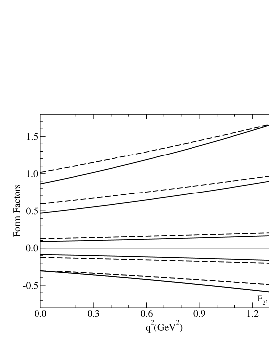
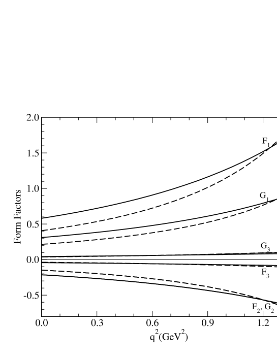
Figure 1: Form factors for $\Lambda_{c}\to\Lambda(1/2^{+})$ obtained using harmonic oscillator wave functions (left panel, HOSR and HONR models) and Sturmian wave functions (right panel, STSR and STNR models). In each panel, the solid curves arise from the semirelativistic version of the model, while the dashed curves arise from the nonrelativistic version. Note that $F_{2}$ is indistinguishable from $G_{2}$ in all cases.

Figure 1 shows the $q^{2}$ dependence of the form factors for the elastic transition $\Lambda_{c}\to\Lambda(1/2^{+})$, calculated in the HONR and HOSR models on the left, and in the STSR and STNR models on the right. In each panel, the solid curves arise from the SR version of the model, while the dashed curves are from the NR version. If we compare the form factors shown in Figure 1, we see that those calculated using the Sturmian wave functions have larger slopes near the non-recoil point (maximum $q^{2}$) than those calculated using the harmonic oscillator wave functions. The form factors calculated in the different models all have similar values near the non-recoil point (as seen in Table 6). The larger slopes in the case of the Sturmian model form factors means that we can expect smaller integrated rates from the STSR and STNR models.

The differential decay rates, $d\Gamma/dq^{2}$, that we obtain in the four models are shown in Figure 2. For these rates, we use $|V_{cs}|=0.974$. In these figures, we show the differential rates for decays to the elastic channel, as well as for two orbital excitations, the states with $J^{P}=1/2^{-}$ and $3/2^{-}$. We have also examined the differential decay rates to the $3/2^{+}$ and $5/2^{+}$ orbitally excited states, as well as to the $1/2^{+}$ radially excited state. With the exception of the latter, we find these rates to be significantly smaller than those shown in this figure.

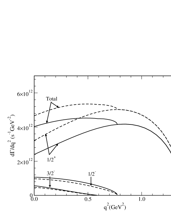
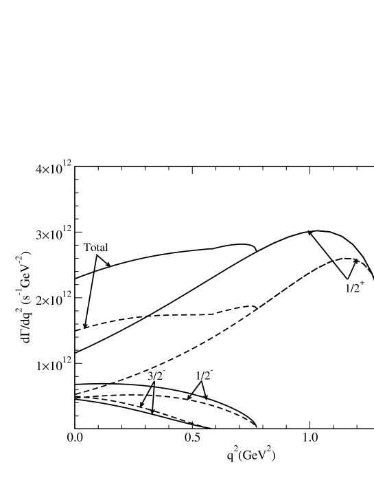
Figure 2: The differential decay rates for different $\Lambda_{c}\to\Lambda^{(*)}$ transitions, in the different models that we use. The curves on the left arise from the two versions of the harmonic oscillator model, while those on the right are from the Sturmian models. The curves are for exclusive final states with $J^{P}=1/2^{+}$, $1/2^{-}$ and $3/2^{-}$. Also shown are the differential decay rates obtained by adding the exclusive modes described (labeled as ‘total’). In each panel, the solid curves arise from the semirelativistic versions of the models, while the dashed curves arise from the nonrelativistic versions.

As expected from the plots for the form factors, the differential decay rates that arise from the Sturmian wave functions for the ground state show a larger variation over the allowed $q^{2}$ range. We also point out that the most noticeable difference between the NR and SR versions of a particular model is seen in the differential rate for the elastic decay.

The integrated decay rate for the different final states in the different models are shown in Table 8. As anticipated above, the total semileptonic decay rates that we obtain in the harmonic oscillator models are significantly larger than those obtained in the Sturmian models. This effect is largest in the elastic decays, where the HO models predict decay rates that are more than twice as large as the ST models. We note that the elastic rates predicted by the ST models are much closer to the experimentally reported rate CLEO than those predicted by the HO models.

Table 8: Integrated decay rates for $\Lambda_{c}\to\Lambda^{(*)}$ in units of $10^{11}s^{-1}$, for different $\Lambda$ states in the four models we consider. The last row shows the ‘elastic fraction’ obtained in our model, where the decays shown in the table are assumed to saturate the semileptonic decays.

Spin	$\Gamma$(HONR)	$\Gamma$(HOSR)	$\Gamma$(STNR)	$\Gamma$(STSR)	Expt. CLEO
$1/2^{+}$	$2.10$	$2.36$	0.79	1.11	1.05$\pm$ 0.35
$1/2^{-}$	$0.19$	$0.29$	0.12	0.15	-
$3/2^{-}$	$0.05$	$0.06$	0.06	0.05	-
$1/2^{+}_{1}$	$0.02$	$0.02$	$<$0.01	$<$0.01	-
total	2.36	2.73	0.97	1.31	-
$\Gamma_{\Lambda}/\Gamma_{\rm total}$	0.89	0.86	0.81	0.85	1.0 (assumed)

From Table 8, it is clear that, while the elastic channel dominates the decay rate of the $\Lambda_{c}$, it does not saturate the decay. In each model, we find that the decay rate to the $1/2^{-}$ state is roughly one tenth of the elastic decay rate, while the decay rate to the $3/2^{-}$ state is about five percent of the elastic. Decays to these two excited states account for about 15% of the total decays of the $\Lambda_{c}$, assuming that decays to other excited states are negligible. It is also interesting to note that the ratio $\Gamma_{\Lambda}/\Gamma_{\rm total}$ is almost independent of the model that we use, even though the absolute rates are very different in the different models.

The assumption that the channels we explore saturate the resonant decays of the $\Lambda_{c}$ is certainly consistent with the results we have obtained with the other states that we consider. First we point out that phase space limits how many excited $\Lambda$ states can be considered, and the higher the excitation, the more limited the phase space available for producing such a state. For some final states for which there might be sufficient phase space to allow the decay, the spin-space structure of the state allows little overlap with the initial baryon, and configuration mixing that could involve components with larger overlap with the initial baryon is very small. In addition, angular momentum factors (in orbitally excited states) lead to suppression of the decay rate.

We can compare our predictions for decays to the excited $\Lambda$ states with the assumption made by the CLEO Collaboration CLEO , that the elastic channel saturates the semileptonic decays of the $\Lambda_{c}$. In our models, we find that between 11% and 19% of the $\Lambda_{c}$ semileptonic decays are to excited states. In addition, our branching fraction (of 81% to 89%) to the ground state $\Lambda$ must represent an upper limit, as we have not included any non-resonant production of multi-particle final states. It appears difficult to understand the lack of evidence for any decays to excited states in Ref. CLEO . This article reports no signal for decays of the kind $\Lambda_{c}\to\Lambda Xe^{+}\nu$, and this is taken as evidence of saturation. However, the excited $\Lambda$ states that we consider do not decay to $\Lambda\pi$, the most obvious decay mode to search for, as this decay is isospin violating. They will predominantly decay to $\Sigma\pi$ final states. In fact, the $1/2^{-}$ state, the $\Lambda(1405)$, has a 100% branching fraction to $\Sigma\pi$, while the $\Lambda(1520)$, the $3/2^{-}$ state, has roughly equal dominant branching ratios to $\Sigma\pi$ and $NK$, with only about ten percent going into $\Lambda\pi\pi$. Thus, our suggestion is that CLEO should investigate final states like $\Sigma\pi\ell\nu$ and $NK\ell\nu$, and not states like $\Lambda\pi\pi\ell\nu$.

The results discussed above are obtained using the assumption that the lightest of the $J^{P}=1/2^{-}$ $\Lambda$ states, identified with the $S_{01}$ state $\Lambda(1405)$ found in analyses of scattering data, is a three-quark state. There are a number of other descriptions of this state in the literature, such as a dynamically generated bound state oset , and a multi-quark state choe . If the CLEO Collaboration (or other groups) search for decays of the $\Lambda_{c}$ to excited $\Lambda$ states, especially the $\Lambda(1405)$, and find no such decays, this would be a strong hint that this state is not a simple three quark state, as we have assumed.

Our estimate of the fraction of $\Lambda_{c}$ decays to excited states has important consequences for the absolute normalization of the branching fractions to the more than sixty observed final states in $\Lambda_{c}^{+}$ decay. Most of these branching fractions are measured relative to the decay mode $\Lambda_{c}^{+}\to pK^{-}\pi^{+}$, and the absolute branching fraction of this mode cannot be extracted from data without introducing model dependence. One of the two important techniques for this extraction is based on measurements Argus96 ; CLEO91 of the cross section for $\Lambda_{c}^{+}X$ production in $e^{+}e^{-}$ annihilation, with the subsequent semileptonic decay $\Lambda_{c}^{+}\to\Lambda\ell^{+}\nu_{\ell}$. The extraction relies on the assumption that the fraction $f$ of decays $\Lambda_{c}^{+}\to X_{s}\ell^{+}\nu_{\ell}$ that have $X_{s}$ as the ground state $\Lambda$ is unity (the elastic channel saturates the semileptonic decays), with a significant uncertainty. Our calculated value $f=0.85$, with an error of $0.04$ estimated by evaluating $f$ in four different models, changes the central value of this parameter and may allow a reduction in the assumed error from model dependence in the extracted absolute branching fractions.

VI.2.2 $\Lambda_{b}\to\Lambda_{c}^{(*)}$

In Table 9 we show the values of the form factors at the non-recoil point, for the decays $\Lambda_{b}\to\Lambda_{c}^{(*)}$, where this notation means that the $\Lambda_{c}$ may be in an excited state. The results from all four models are shown, along with the results from a lattice study Richards . The lattice results are actually given as multiples of $\xi(w)$, evaluated at the non-recoil point, and Ref. Richards reports a number of different values for $\xi(w)$. In the ‘physical’ limit, values $\xi^{(A)}(1)=1.03^{+0.18}_{-0.19}$ and $\xi^{(V)}(1)=0.87\pm 0.22$ are quoted, where the two extractions are from the axial and vector currents, respectively. The results we obtain for the elastic decays are consistent with the predictions of HQET as estimated by Scora scora , as well as with these lattice simulations.

Table 9: Form factors of $\Lambda_{b}\to\Lambda_{c}^{(*)}$, calculated at the non-recoil point, in the four models we use. Also shown are the lattice estimates for the elastic form factors, taken from Richards . The lattice numbers are in fact multiples of their estimate of $\xi(w)$, for which they explore a number of scenarios.

$J^{P}$	model	$F_{1}$	$F_{2}$	$F_{3}$	$F_{4}$	$G_{1}$	$G_{2}$	$G_{3}$	$G_{4}$
$1/2^{+}$	HONR	1.27	-0.20	-0.08	-	0.99	-0.20	0.08	-
$1/2^{+}$	HOSR	1.24	-0.18	-0.08	-	0.97	-0.18	0.08	-
$1/2^{+}$	STNR	1.28	-0.26	-0.04	-	0.98	-0.26	0.04	-
$1/2^{+}$	STSR	1.20	-0.22	-0.03	-	0.92	-0.22	0.03	-
$1/2^{+}$	Lattice	1.28$\pm$0.06	-0.19$\pm$0.04	-0.06${}^{+0.02}_{-0.01}$	-	0.99	-0.24${}^{+0.05}_{-0.04}$	0.09$\pm 0.02$	-
$1/2^{-}$	HONR	0.12	-1.20	0.11	-	1.21	-1.05	0.03	-
$1/2^{-}$	HOSR	0.15	-0.95	0.09	-	1.01	-0.82	0.04	-
$1/2^{-}$	STNR	0.10	-1.63	0.14	-	1.61	-1.50	0.03	-
$1/2^{-}$	STSR	0.11	-1.21	0.10	-	1.24	-1.12	0.03	-
$3/2^{-}$	HONR	-1.33	0.17	0.13	-0.06	-1.03	0.17	-0.13	0.06
$3/2^{-}$	HOSR	-1.13	0.15	0.12	-0.05	-0.87	0.15	-0.12	0.05
$3/2^{-}$	STNR	-1.75	0.25	0.15	-0.05	-1.36	0.25	-0.22	0.05
$3/2^{-}$	STSR	-1.31	0.16	0.11	-0.05	-1.04	0.16	-0.18	0.05

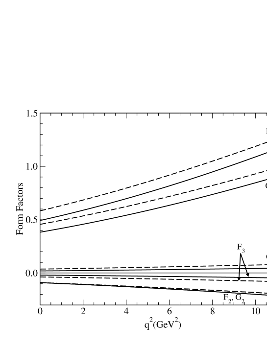
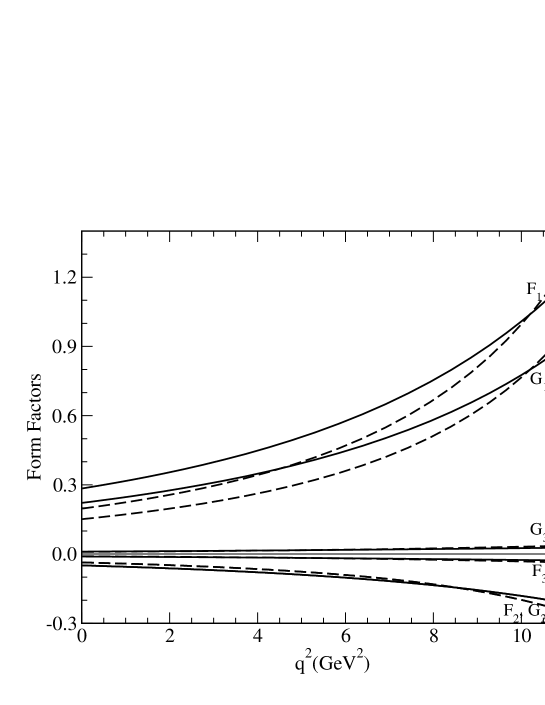
Figure 3: Form factors for $\Lambda_{b}\to\Lambda_{c}(1/2^{+})$ obtained using harmonic oscillator wave functions (left panel, HOSR and HONR models) and Sturmian wave functions (right panel, STSR and STSR models). In each panel, the solid curves arise from the semirelativistic version of the model, while the dashed curves arise from the nonrelativistic version. Note that $F_{2}$ is indistinguishable from $G_{2}$ in all cases.

Figure 3 shows the $q^{2}$ dependence of the form factors for the elastic decay of the $\Lambda_{b}$, calculated in the HONR and HOSR models on the left, and in the STSR and STNR models on the right. In each panel, the solid curves arise from the SR version of the model, while the dashed curves are from the NR version. As we noted in the case of the $\Lambda_{c}\to\Lambda(1/2^{+})$, the form factors obtained in the Sturmian basis have significantly larger slopes than the corresponding form factors calculated in the harmonic oscillator basis, at the non-recoil point.

In terms of the Isgur-Wise function $\xi(w)$ for the elastic decay of the $\Lambda_{b}$, the form factor $F_{1}$ is

$$F_{1}=\left[1+\bar{\Lambda}\left(\frac{1}{2m_{c}}+\frac{1}{2m_{b}}\right)\right]\xi(w),$$ (62)

where $\bar{\Lambda}=m_{\Lambda_{b}}-m_{b}=m_{\Lambda_{c}}-m_{c}$ at leading order in the heavy quark expansion. From the forms given in Appendix C, and with the identification $\bar{\Lambda}\approx 2m_{\sigma}$, we can extract

$$\xi(w)\approx\exp\left(-\frac{3m^{2}_{\sigma}}{2m^{2}_{\Lambda_{c}}}\frac{p^{2}}{\alpha^{2}}\right)$$ (63)

in the harmonic oscillator basis, or

$$\xi(w)\approx\frac{1}{\left[1+\frac{3m^{2}_{\sigma}}{2m^{2}_{\Lambda_{c}}}\frac{p^{2}}{\beta^{2}}\right]^{2}}$$ (64)

in the Sturmian basis (assuming single-component wave functions), and we have assumed that $\alpha_{\lambda}=\alpha_{\lambda^{\prime}}\equiv\alpha$, $\beta_{\lambda}=\beta_{\lambda^{\prime}}\equiv\beta$ in the heavy quark limit. Writing

$$p^{2}=m_{\Lambda_{c}}^{2}(w^{2}-1)\approx 2m_{\Lambda_{c}}^{2}(w-1),$$ (65)

the above expressions become

$$\xi(w)\approx\exp\left(-\frac{3m^{2}_{\sigma}}{\alpha^{2}}(w-1)\right)$$ (66)

in the harmonic oscillator basis, or

$$\xi(w)\approx\frac{1}{\left[1+\frac{3m^{2}_{\sigma}}{\beta^{2}}(w-1)\right]^{2}}$$ (67)

in the Sturmian basis.

The Isgur-Wise function may be expanded as

$$\xi(w)=1-\rho^{2}(w-1)+\frac{\sigma^{2}}{2}(w-1)^{2}+\dots,$$ (68)

where the slope of the form factor at the non-recoil point has been denoted $\rho^{2}$, and the curvature is denoted $\sigma^{2}$. Rigorous bounds have been placed on the values of both the slope and curvature parameters for meson decays, and some models have difficulty in satisfying those bounds. In particular, in the model of ISGW ISGW , a factor $\kappa$ was introduced by hand (see the discussion between Eqs. (B2) and (B3) of Ref. ISGW ) to modify the $q^{2}$ dependence of the form factors. In our model, the equivalent procedure would be to change $I_{H}$ in Eq. (C.1.1) from

$$I_{H}=\left(\frac{\alpha_{\lambda}^{3/2}\alpha_{\lambda^{\prime}}^{3/2}}{\alpha_{\lambda\lambda^{\prime}}^{3}}\right)\exp\left(-\frac{3m^{2}_{\sigma}}{2m^{2}_{\Lambda_{q}}}\frac{p^{2}}{\alpha_{\lambda\lambda^{\prime}}^{2}}\right)$$

as calculated to

$$I_{H}=\left(\frac{\alpha_{\lambda}^{3/2}\alpha_{\lambda^{\prime}}^{3/2}}{\alpha_{\lambda\lambda^{\prime}}^{3}}\right)\exp\left(-\frac{3m^{2}_{\sigma}}{2m^{2}_{\Lambda_{q}}}\frac{p^{2}}{\kappa^{2}\alpha_{\lambda\lambda^{\prime}}^{2}}\right).$$

The argument used by ISGW was that this factor of $\kappa$ would take into account ‘relativistic effects’. The effect of this change is shown in Figure 4, where the form factors for $\Lambda_{b}\to\Lambda_{c}$ are plotted as functions of $w=v\cdot v^{\prime}$, for the two harmonic oscillator models (upper graphs). For comparison, the lower graph shows form factors obtained in the Sturmian basis, also as functions of $w$. The graph on the upper left shows our calculated form factors, while that on the upper right shows form factors including the factor of $\kappa$.

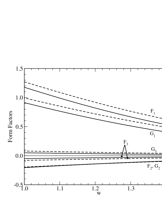
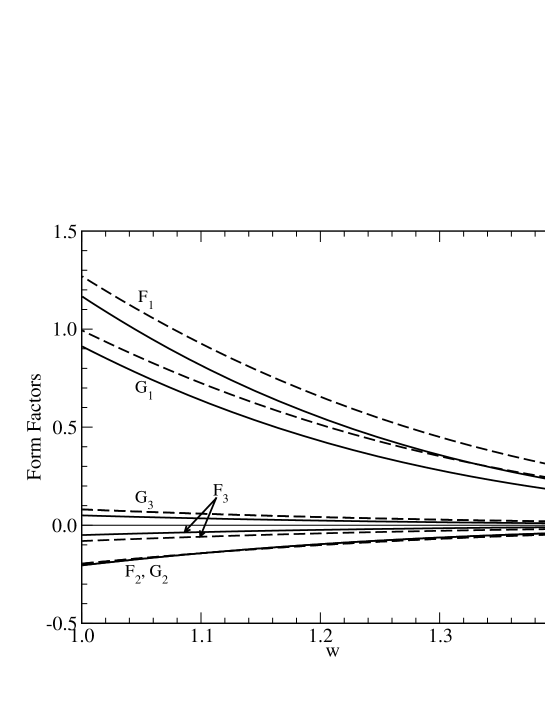
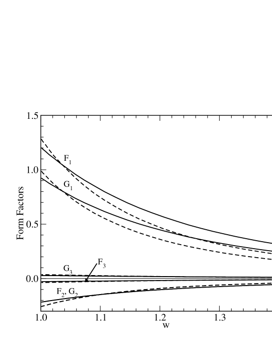
Figure 4: The elastic form factors for the decay of the $\Lambda_{b}$ as functions of $w$. The upper two graphs arise from the harmonic oscillator model, while the lower graph is from the Sturmian version of our model. Among the upper graphs, the panel on the left shows the form factors obtained in this work, while those on the right incorporate a ‘relativistic’ factor in the exponential (see text). In each panel, the solid curves arise from the semirelativistic version of the model.

Table 10 lists the slope of the Isgur-Wise function that we have extracted, at the non-recoil point, in both the harmonic oscillator and Sturmian models, as well as in the ‘relativistically modified’ harmonic oscillator model (using the factor $\kappa$). The slopes of the form factor near the non-recoil point are larger in the Sturmian models than in the harmonic oscillator models. This is easily understood by noting that the value of $\rho^{2}$ is

$$\rho^{2}=3\frac{m_{\sigma}^{2}}{\alpha^{2}}$$ (69)

in the HO models, and

$$\rho^{2}=6\frac{m_{\sigma}^{2}}{\beta^{2}}$$ (70)

in the ST models. The extra factor of two in the latter case arises because the form factors in the ST models have a dipole dependence on $w$. A corresponding monopole form would give the same slope as the HO models. Since the values of $m_{\sigma}$ are similar in the two sets of models, and the values of $\alpha$ are not very different from the values of $\beta$, the ST models will give slopes that are roughly twice as large as the HO models. In the same way, it is easily shown that the ST models lead to curvatures that are about six times as large as those obtained in the HO models.

Table 10: Slope of the Isgur-Wise function, evaluated at the non-recoil point, for the elastic decay of the $\Lambda_{b}$.

model	HONR	HOSR	HONR$\kappa$	HOSR$\kappa$	STNR	STSR
$d\xi(w)/dw$	-1.38	-1.33	-2.82	-2.71	-5.71	-3.27

The $\kappa$-modified harmonic oscillator model leads to slopes that are similar to those obtained in the Sturmian models, since the value chosen for $\kappa$ was 0.7 (so that $1/\kappa^{2}\approx 2$). Relativistic effects do not need to be invoked to obtain the large slopes obtained in the Sturmian models. The differences in the slopes are simply artifacts of the expansion bases used for the wave functions.

In the follow-up article to Ref. ISGW , Scora and Isgur isgw2 rewrite the quark model form factors, explicitly replacing the exponential factor that arises with the harmonic oscillator wave functions. The change they make is

$$\exp\left\{-\frac{1}{6}r^{2}_{\rm wf}[(m_{B}-m_{D})^{2}-q^{2}]\right\}\longrightarrow\frac{1}{\left\{1+\frac{1}{6N}r^{2}[(m_{B}-m_{D})^{2}-q^{2}]\right\}^{N}},$$ (71)

where $r^{2}_{\rm wf}$ is the value obtained from the harmonic oscillator wave functions, and

$$r^{2}=\frac{3}{4m_{Q}m_{q}}+r^{2}_{\rm wf}+r^{2}_{\rm QCD},$$ (72)

where the last term arises from matching of currents in HQET with full QCD. In Eq. (71), the integer $N=2+n+n^{\prime}$, where $n$ and $n^{\prime}$ are the harmonic oscillator principal quantum numbers for the initial and final wave functions. The final forms that they used are therefore very similar to the forms that we have obtained in the Sturmian models.

The values we have obtained for the slope of the Isgur-Wise function in our Sturmian models are significantly larger than the value obtained recently by Huang et al. huang using a HQET approach based on QCD sum rules: their value for $\rho^{2}$ is less than 1.5, similar to the values we obtain in the HO models. In a recent analysis of the $\Lambda_{b}$ form factor measured in hadronic Z decays, the DELPHI Collaboration delphi found $\rho^{2}=2.03\pm 0.46$, where the error shown is statistical. They also reported two sets of systematic errors, each comparable to the statistical error. This result means that for the Sturmian models, we will obtain integrated decay rates that are significantly smaller than the DELPHI rate. In the lattice study by Bowler et al. Richards , the reported slopes is $1.1\pm 1.0$. A more recent lattice study with ${\cal O}\left(a^{2},\alpha_{s}a^{2}\right)$ improved lattices gottlieb does not quote values for the slope. However, a conservative estimate from the graphs they present gives values for $\rho^{2}$ that appear to be consistent with the large values we obtain in the ST models.

Also of some interest is the curvature of the Isgur-Wise function, denoted $\sigma^{2}$. In the HO models with no modifications, the prediction is that $\sigma^{2}_{\rm HO}=(\rho^{2}_{\rm HO})^{2}$, while the ST models give $\sigma^{2}_{\rm ST}=3(\rho^{2}_{\rm ST})^{2}/2$. Bounds on the curvature of the Isgur-Wise function for meson decays have been derived by Le Yaouanc, Oliver and Raynal curvature . To the best of our knowledge, no such bounds have been derived for baryon decays. However, the values of the curvature we obtain using both the HO and ST models easily satisfy the known bounds for meson decays. Note that the large slope and large curvature we obtain suggest that the common procedure of parameterizing the Isgur-Wise function only in terms of its slope parameter, can potentially lead to significant errors in the extraction of CKM matrix elements.

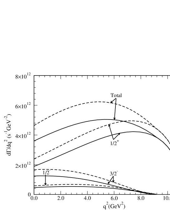
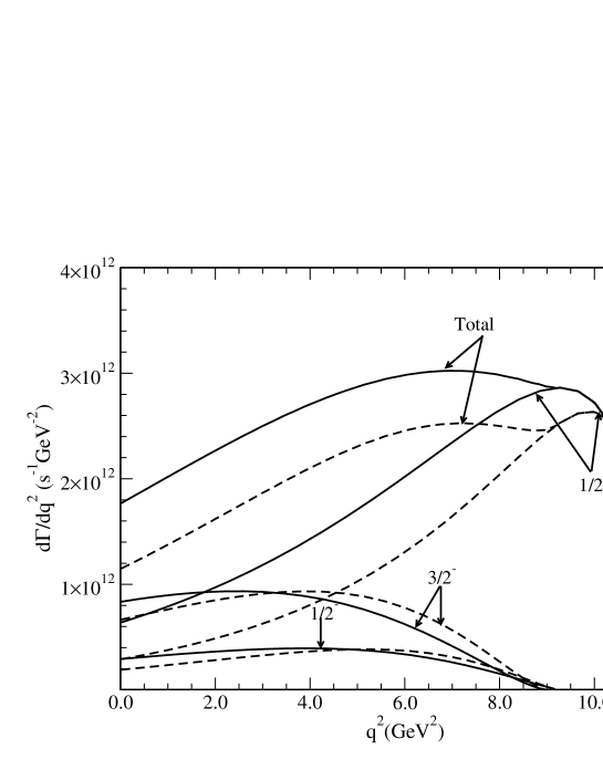
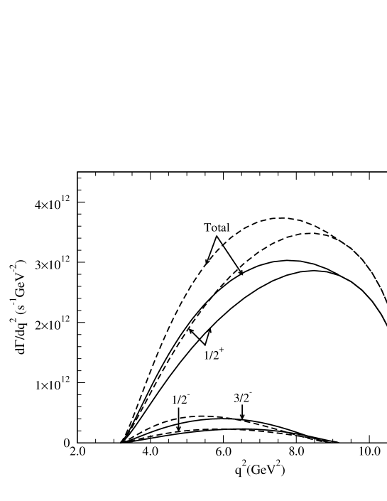
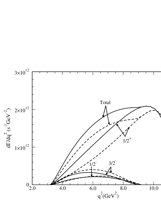
Figure 5: The differential decay rates for different $\Lambda_{b}\to\Lambda_{c}^{(*)}$ transitions, in the various models that we use. The curves on the left arise from the two versions of the harmonic oscillator model, while those on the right are from the Sturmian models. The upper panels are for $\Lambda_{b}\to\Lambda_{c}^{(*)}\ell\bar{\nu}_{\ell}$, where $\ell$ is $e^{-}$ or $\mu^{-}$. The lower panels are for $\Lambda_{b}\to\Lambda_{c}^{(*)}\tau\bar{\nu}_{\tau}$. The curves are for final states with $J^{P}=1/2^{+}$, $1/2^{-}$ and $3/2^{-}$.

The differential decay rates $d\Gamma/dq^{2}$ that we obtain in the four models are shown in Figure 5 (assuming $|V_{cb}|=.041$). In these plots, we show the differential rates for the elastic channel, for the radially excited $1/2^{+}_{1}$ state, as well as for decays to two orbital excitations, the states with $J^{P}=1/2^{-}$ and $3/2^{-}$. We have also examined the decay rates to the $3/2^{+}$, $5/2^{+}$ states, and found them to be smaller than those shown in this figure, contributing of the order of one or two percent to the total rate.

The integrated decay rate for the different final states in the different models are shown in Table 11. As anticipated above, the total semileptonic decay rates that we obtain in the harmonic oscillator models are significantly larger than those obtained in the Sturmian models. This effect is largest in the elastic decays, where HO models predict decay rates that are more than twice as large as the ST models. Note that, in all models, the decay rate to the $3/2^{-}$ state is roughly twice the decay rate to the $1/2^{-}$ state. In the heavy quark limit, this ratio of decay rates is expected to be two, and results from arguments that are similar to spin-counting arguments.

Table 11: Rates for $\Lambda_{b}\to\Lambda_{c}^{(*)}$ decays in units of $10^{10}s^{-1}$. The first five rows are for decays with a muon or electron in the final state, while the last four rows are for decays with a $\tau$ in the final state. The rows labeled ‘total’ are obtained by adding the exclusive decay rates shown in the table, while the row with the branching fractions assumes that the exclusive channels shown saturate the semileptonic decays of the $\Lambda_{b}$. The elastic fraction reported by the DELPHI collaboration (fifth row, sixth column) is actually $\frac{\Gamma(\Lambda_{b}\to\Lambda_{c}\ell\bar{\nu}_{\ell})}{\Gamma(\Lambda_{b}\to\Lambda_{c}\ell\bar{\nu}_{\ell})+\Gamma(\Lambda_{b}\to\Lambda_{c}\pi\pi\ell\bar{\nu}_{\ell})}$. The errors on both DELPHI results are statistical and systematic, respectively.

$J^{P}$	$\Gamma$(HONR)	$\Gamma$(HOSR)	$\Gamma$(STNR)	$\Gamma$(STSR)	$\Gamma_{\rm DELPHI}$
$1/2^{+}$	$4.60$	$5.39$	1.47	2.00	$4.07^{+0.90+1.30}_{-0.65-0.98}$
$1/2^{-}$	$0.45$	$0.52$	0.26	0.27	-
$3/2^{-}$	$0.95$	$0.91$	0.63	0.61	-
Total ($\Lambda_{c}^{(*)}\ell^{-}\bar{\nu}_{\ell}$)	5.95	6.82	2.36	2.88	-
$\Gamma_{\Lambda_{c}}/\Gamma_{\rm total}$	0.76	0.79	0.62	0.69	$0.47^{+0.10+0.07}_{-0.08-0.06}$
$1/2^{+}$	$1.90$	$2.09$	0.82	1.00	-
$1/2^{-}$	$0.10$	$0.11$	0.08	0.07	-
$3/2^{-}$	$0.15$	$0.13$	0.14	0.12	-
Total ($\Lambda_{c}^{(*)}\tau^{-}\bar{\nu}_{\tau}$)	2.15	2.33	1.04	1.19	-

Table 11 also shows that a significant fraction of the semileptonic decay of the $\Lambda_{b}$ is inelastic. This is analogous to what has been seen in $B$ semileptonic decays, where the elastic channels account for no more than about 80% of the total semileptonic decay rate. For the $\Lambda_{b}$, our predicted ratios are similar, ranging from 62% to 77% of the total semileptonic decay rate. We have estimated the total semileptonic decay rate by assuming that the three exclusive modes shown in Table 11 saturate the semileptonic decays (rates to other states that we have examined are significantly smaller than those shown in the table). Using these numbers, we obtain predictions for the total semileptonic decay rate of the $\Lambda_{b}$, also shown in Table 11.

For comparison, the PDG pdg gives a rate of $7.486\pm 2.105\times 10^{10}s^{-1}$ for the inclusive semileptonic decay $\Lambda_{b}\to\Lambda_{c}\ell\bar{\nu}+$ anything. This is significantly larger than any of the total semileptonic widths we obtain, but the authors of the PDG emphasize that this value results from assumptions about the fragmentation of $b$ quarks into baryons, and ‘cannot be thought of as measurements’ pdg . The DELPHI value for the elastic semileptonic decay rate is also shown in Table 11. As anticipated, the rates we obtain in the Sturmian models are significantly smaller than the DELPHI rate, while those obtained in the harmonic oscillator models are consistent with the DELPHI measurement.

The above examination of the decays of the $\Lambda_{c}$ found that the Sturmian models provided rates that were consistent with the CLEO measurements, while the harmonic oscillator models gave rates that were twice as large. This suggested that the Sturmian models might be more reliable. For the $\Lambda_{b}$ decays, we see that the harmonic oscillator models provide rates that are more consistent with the single measurement available to date. For the Sturmian models, the predicted rates are about 2$\sigma$ away from the reported value, if the systematic and statistical errors are treated in quadrature.

The DELPHI Collaboration also reported on the elastic fraction of the semileptonic decays of the $\Lambda_{b}$. For the ratio $\frac{\Gamma(\Lambda_{b}\to\Lambda_{c}\ell\bar{\nu}_{\ell})}{\Gamma(\Lambda_{b}\to\Lambda_{c}\ell\bar{\nu}_{\ell})+\Gamma(\Lambda_{b}\to\Lambda_{c}\pi\pi\ell\bar{\nu}_{\ell})}$, they find a value of $0.47^{+0.10+0.07}_{-0.08-0.06}$, with no evidence for resonant decays. This ratio is smaller than we predict, in all models. However, our predictions must be thought of as upper limits for the elastic fraction, as we do not include any non-resonant semileptonic decays. We note that our predicted ratios are already somewhat smaller than those reported in the decays of $B$ mesons, while the DELPHI ratio is smaller still, suggesting that there are significant differences between the semileptonic decays of the heavy baryons and those of the heavy mesons. If the DELPHI results for both for the elastic rate and the elastic fraction are not modified by future experiments, this aspect of the physics of heavy hadrons will require further scrutiny.

VI.2.3 $\Lambda_{Q}\to N^{(*)}$ Decay

The decays of the $\Lambda_{Q}$ to final states consisting solely of light quarks are interesting as they provide an alternate means of extracting CKM matrix elements like $V_{ub}$. The expectation from HQET is, modulo $1/m_{Q}$ effects, that the form factors that describe the $\Lambda_{c}\to n$ semileptonic decays will be the same as those describing the $\Lambda_{b}\to p$ semileptonic decays. To explore this, we now examine the form factors for these two decays.

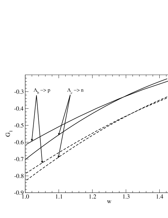
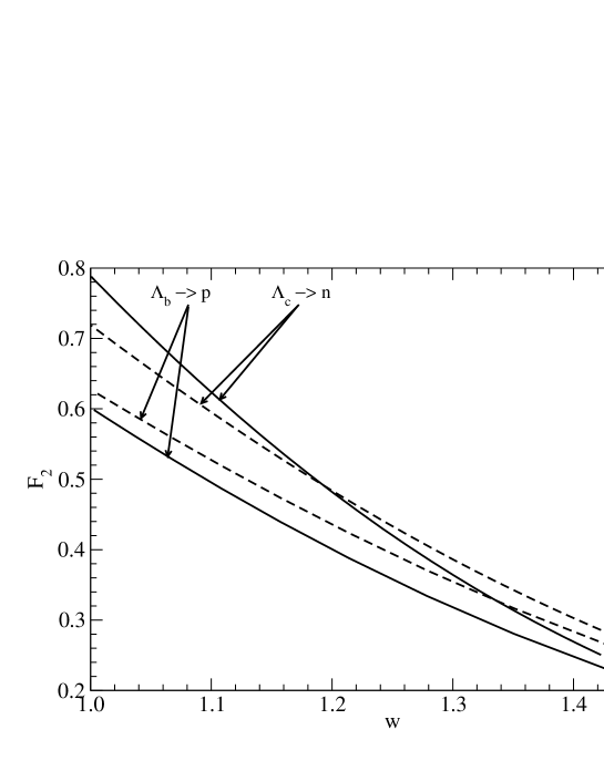
Figure 6: Form factors $\xi_{1}^{(V)}$ (top left), $\xi_{1}^{(A)}$ (top right) and $\xi_{2}$ (bottom) for the transitions $\Lambda_{c}\to n$ and $\Lambda_{b}\to p$. All curves are found using the harmonic oscillator models, with the solid curves corresponding to HOSR, and the dashed curves to HONR. The two plots for $\xi_{1}$ arise from the two ways of evaluating this form factor, shown in Eq. (VI.2.1).

In Figure 6 we show the form factors $\xi_{1}^{(V)}$, $\xi_{1}^{(A)}$ and $\xi_{2}$ for the transitions $\Lambda_{c}\to n$ and $\Lambda_{b}\to p$, obtained in the two harmonic oscillator models. The two forms $\xi_{1}^{(V,A)}$ are found using the two sets of equations in Eq. (VI.2.1). The value of $\xi_{2}$ is independent of which of the two sets of equations we use, up to the order to which we calculate the form factors. In both the nonrelativistic and semirelativistic versions of the model, the two curves for $\xi_{1}^{(A)}$ (top right plot in Fig. 6) are very similar, indicating that the HQET prediction, that this form factor should be the same for both transitions, indeed holds up to small corrections. For the semirelativistic version, the two curves are closer than in the nonrelativistic case. The differences seen in the curves for $\xi_{2}$, which are consistent with those in the curves for $\xi_{1}^{(A)}$, arise mainly from the differences in the size parameters ($\alpha_{\rho}$ and $\alpha_{\lambda}$) between the $\Lambda_{c}$ and $\Lambda_{b}$ states in the models (see Table 2). The curves for $\xi_{1}^{(V)}$ (top left plot in Fig. 6) show the biggest differences in going from $\Lambda_{b}\to p$ to $\Lambda_{c}\to n$, in both models. Here, the differences get some contribution from the $1/m_{Q}$ term that is present in $F_{1}$.

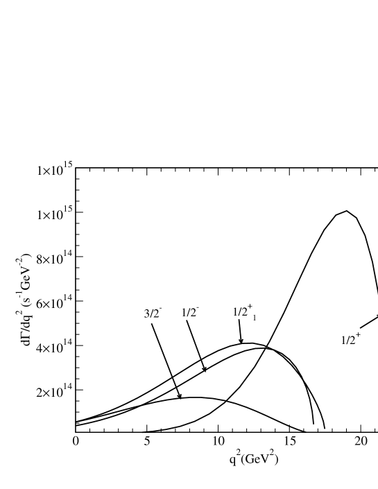
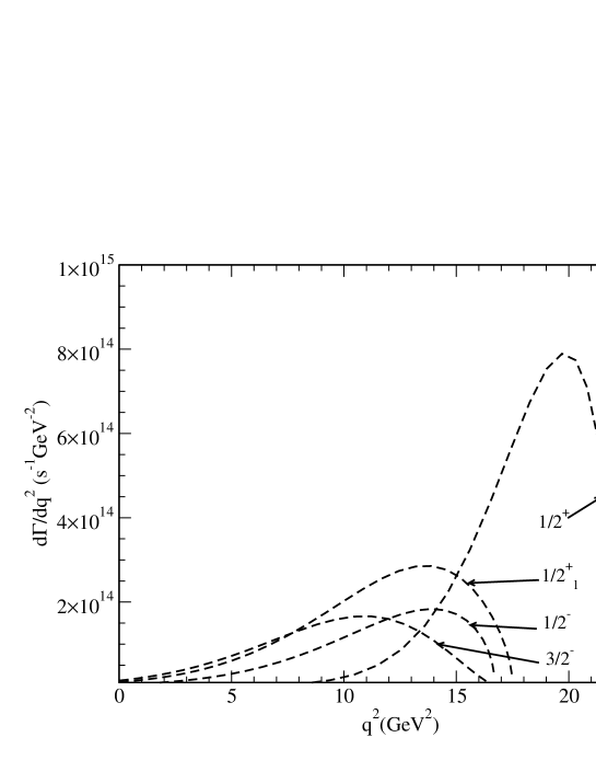
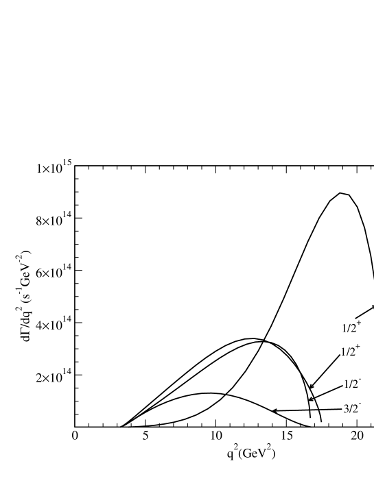
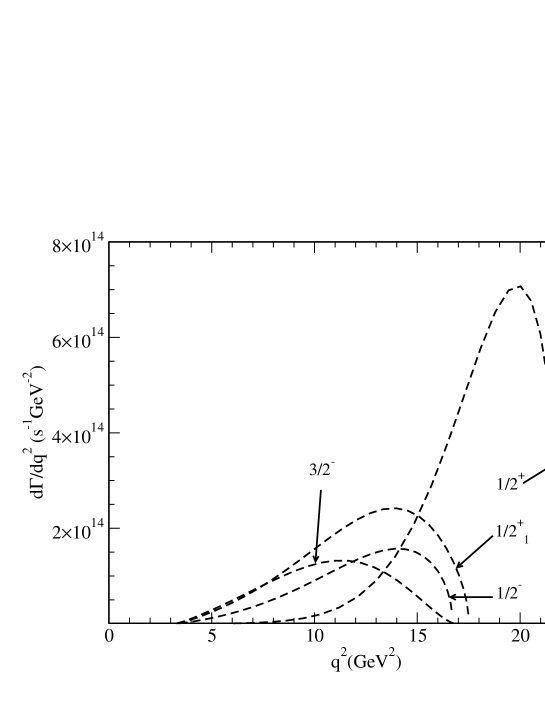
Figure 7: Differential decay rates for $\Lambda_{b}\to N^{(*)+}$ in the HONR and HOSR models. The upper panels show the rates for $\Lambda_{b}\to N^{(*)+}e^{-}\bar{\nu}_{e}$, while the lower panels show the rates for $\Lambda_{b}\to N^{(*)+}\tau^{-}\bar{\nu}_{\tau}$, both in units of $|V_{ub}|^{2}$. The panels on the left are from the HOSR model, while those on the right are from the HONR model.

In Figure 7, we show the differential decay rates for $\Lambda_{b}$ decaying semileptonically into the four lowest-lying nucleon states, while Table 12 shows the integrated rates into six exclusive states. Also shown in this figure and table are the rates that we obtain when the final lepton is a $\tau$. The ground state nucleon is the largest of the CKM suppressed decays of the $\Lambda_{b}$, but it accounts for less than 50% of these decays, in both of the harmonic oscillator models. A large fraction (about 20%) goes into the first excited state, the Roper resonance, usually treated as a radial excitation of the ground-state nucleon, as it is in this model. As with the $\Lambda(1405)$ in the decays of the $\Lambda_{c}$, this result hinges on the assumption that the Roper resonance is a three-quark state, and that it is the first radial excitation of the nucleon. A number of hypotheses for the internal structure of this state have been made, such as pentaquark partner jaffewilczek , dynamically generated state krehl , and hybrid state kisslinger . In each of these scenarios, the rate at which the $\Lambda_{b}$ decays semileptonically into this state is affected by its internal structure. For the three-quark, radially-excited scenario, the prediction is that decays to this state are about 60% of the decays to the ground state nucleon, a rather large fraction. If ample $\Lambda_{b}$’s can be produced, their semileptonic decays may therefore provide information that can be used in understanding the structure of the Roper resonance.

We have examined decays to other excited nucleons, and those shown in Table 12 are by far the dominant ones. We have also examined one additional $1/2^{+}$ nucleon state, two additional nucleon states with $J^{P}=3/2^{+}$, and one additional nucleon state with $J^{P}=5/2^{+}$, none of which are shown in Table 12. Of these, the rate to the additional $1/2^{+}$ state is less than 1% of the ‘total’ rate that we have estimated, while rates to the additional $3/2^{+}$ and $5/2^{+}$ states are similarly small or even smaller. These small rates are a direct consequence of the structure of these states, as their overlaps with the decaying $\Lambda_{b}$, in the spectator assumption, are very small. The only other excited nucleons that may occur with ‘significant’ rate in the semileptonic decays of the $\Lambda_{b}$ are those with higher spins, such as $7/2^{+}$ and $5/2^{-}$. However, for such states, orbital angular momentum centrifugal factors will lead to some suppression of the decay rate.

Table 12: Decay rates of $\Lambda_{b}\to N^{(*)+}\ell\bar{\nu}_{\ell}$ in units of $10^{12}s^{-1}\times|V_{ub}|^{2}$. Also shown are the rates for $\Lambda_{c}\to N^{(*)0}\ell^{+}\nu_{\ell}$ in units of $10^{10}s^{-1}$, obtained using $|V_{cd}|=0.224$.

	$\Lambda_{b}\to N^{(*)+}\ell^{-}\bar{\nu}_{\ell}$		$\Lambda_{b}\to N^{(*)+}\tau^{-}\bar{\nu}_{\tau}$
$J^{P}$	$\Gamma$(HONR)	$\Gamma$(HOSR)	$\Gamma$(HONR)	$\Gamma$(HOSR)
$1/2^{+}$	$4.55$	$7.55$	4.01	6.55
$1/2^{+}_{1}$	$2.92$	$4.44$	2.20	3.05
$1/2^{-}$	$1.42$	3.85	1.10	2.73
$3/2^{-}$	$1.54$	$1.82$	1.03	1.07
$3/2^{+}$	$1.03$	2.16	0.28	0.58
$5/2^{+}$	$0.79$	$1.49$	0.38	0.55
Total	12.25	21.31	9.00	15.53
	$\Lambda_{c}\to N^{(*)0}\ell^{+}\nu_{\ell}$		-	-
$1/2^{+}$	$1.02$	$1.35$	-	-
$1/2^{-}$	$0.02$	$0.04$	-	-

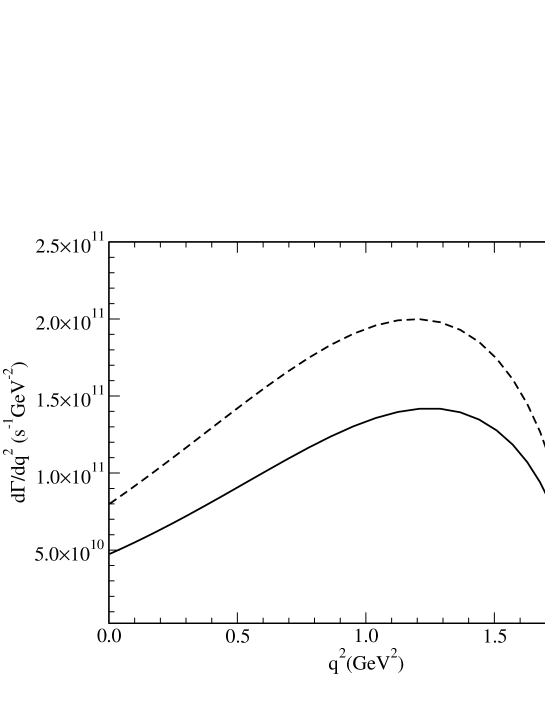
Figure 8: Differential decay rate for $\Lambda_{c}\to n$ in the HONR and HOSR models.

Figure 8 shows the differential decay rate for $\Lambda_{c}\to n$, while the integrated decay rates for two exclusive modes $\Lambda_{c}\to N^{(*)0}$, obtained using $|V_{cd}|=0.224$, are shown in Table 12. It is clear from this table that decays of the $\Lambda_{c}$ to excited states of the nucleon are strongly suppressed, due in part to the reduced phase space.

VII Conclusions and Outlook

A constituent quark model calculation of semileptonic decays of $\Lambda_{b}$ and $\Lambda_{c}$ baryons, which has several novel features, is described here. Analytic results for the form factors for the decays to $J^{P}=1/2^{+}$ ground states and excited states with different quantum numbers are evaluated, and compared to HQET predictions. For $\Lambda_{b}\to\Lambda_{c}$ transitions, the relations among the form factors, predicted by HQET, are satisfied by the form factors obtained in the model, independent of the basis used to describe the baryon wave functions. For the elastic form factors, as well as for the form factors for decays to the $(1/2^{-},\,3/2^{-})$ doublet, the HQET relationships among the form factors are found to hold up to the order we have examined, namely $1/m_{b}$ and $1/m_{c}$. For states of higher spin, we have compared our model form factors to the HQET predictions at leading order, and the expected relations hold at that order.

These form factors depend on the size parameters of the initial and final baryon wave functions, and so a fit to the spectrum of the states treated here is performed. Two model Hamiltonians are used, with either a nonrelativistic or semi-relativistic kinetic energy term, and with Coulomb and spin-spin contact interactions. The wave functions are expanded in either a harmonic oscillator or Sturmian basis, up to second-order polynomials, and our numerical results for form factors and rates are calculated using the resulting mixed wave functions. Four sets of predictions are made for form factors and rates, with wave functions, size parameters and mixing coefficients arising from fits using both the non-relativistic and semi-relativistic Hamiltonians, and using the two different bases. These predictions can be used to assess the model dependence in the results we obtain.

Interestingly, the form factors for decays to ground state daughter baryons evaluated using the Sturmian basis for the wave functions have slopes at the non-recoil point that are significantly larger than those evaluated using the harmonic oscillator basis. As a result, the corresponding integrated decay rates for $\Lambda_{c}\to\Lambda$ elastic decays, calculated using the Sturmian wave functions, are smaller than those obtained using the harmonic oscillator basis wave functions. The Sturmian rates are both consistent within errors with the experimentally reported rate of $1.05\pm 0.35\times 10^{11}$ s^-1, while those calculated using the harmonic oscillator basis are significantly larger. As pointed out by Keister and Polyzou KP , although calculations using the Sturmian basis are not as simple as those using the harmonic oscillator basis, the resulting form factors have shapes which are expansions in inverse powers of $1+k^{2}/\Lambda^{2}$, with $k$ the decay three-momentum (in a non-relativistic decay calculation like ours), and $\Lambda$ a constant which is calculated in terms of quark masses and wave function size parameters. This is closer to the form expected from experimental studies of hadron decay form factors, and so the use of Sturmian basis functions produces realistic results for decay calculations even with the inevitable truncations of the basis required for tractability. Larger scale numerical calculations using the Sturmian basis require fewer basis states than those using the harmonic oscillator basis to yield accurate energies and decay form factors for excited states.

Although the use of a semi-relativistic Hamiltonian does not necessarily lead to a better fit to the spectrum, in calculations using both bases it results in an integrated decay rate for $\Lambda_{c}\to\Lambda$ elastic channel that is closer to the central value that has been experimentally reported. However, the rate obtained in the nonrelativistic version of the Sturmian model is also consistent (within 1 $\sigma$) with the experimentally reported value.

Decay form factors and rates to all available excited state daughter baryons are evaluated using these four models. Significant branching fractions are found for $\Lambda_{c}$ inelastic semileptonic decays in all four calculations, with the total to all excited states ranging from 11 to 19%. This has important consequences for the absolute normalization of the branching fractions to the many observed final states in $\Lambda_{c}^{+}$ decay, most of which are measured relative to the decay mode $\Lambda_{c}^{+}\to pK^{-}\pi^{+}$. The extraction of the absolute branching fraction of this mode, from measurements of the cross section for $\Lambda_{c}^{+}X$ production in $e^{+}e^{-}$ annihilation, requires knowledge of the fraction $f$ of semi-leptonic decays $\Lambda_{c}^{+}\to X_{s}\ell^{+}\nu_{\ell}$ to the elastic channel. This contradicts the available CLEO analyses, in which it is assumed that the elastic decay of the $\Lambda_{c}$ saturates its semileptonic decays. A larger fraction, from 23 to 38%, of $\Lambda_{b}\to\Lambda_{c}$ semileptonic decays, are found to be inelastic. Elastic decays of the $\Lambda_{b}$ involving tau leptons in the final state are suppressed by roughly a factor of two because of the reduction in the final-state phase space, and those to excited baryon states are suppressed more strongly.

HQET predicts that the form factors $\xi_{1}$ and $\xi_{2}$, defined earlier, should be the same for the decays $\Lambda_{b}\to N^{0}$ and $\Lambda_{c}\to N^{+}$, up to $1/m_{b}$ or $1/m_{c}$ corrections. Within our models, we find that the two form factors are very similar, but not identical, with the differences arising from differences in the size parameters for the $\Lambda_{b}$ and $\Lambda_{c}$. In the case of the decay of the $\Lambda_{b}$ to nucleons, we find that the ‘elastic’ fraction is quite small, of the order of 35% when the leptons produced in the decay are light. A number of excited nucleons contribute to the total rate, with the radially excited Roper having the next largest branching fraction. This may be used as a test of the structure of this resonance, if ample $\Lambda_{b}$’s can be produced.

The work presented in this manuscript can be extended in a number of directions. We plan to examine the semileptonic decays of heavy $\Omega_{Q}$ baryons, both to ground states and to a number of excited states, in a calculation similar to the one outlined here. Since the description of these states using both the quark model and HQET is more complex, it will be interesting to see if the correspondence between quark-model results and the predictions of HQET still holds. We can also apply our model to the description of the semileptonic decays of the light baryons, although these are already successfully described by Cabbibo theory. Essentially all experimentally accessible observables for these decays have been measured, and it will be interesting to see if our model, constructed with no special reference to chiral symmetry or current algebra, can describe the results of these measurements.

We have not examined the predictions of our model for the many polarization observables which can, in principle, be measured in semileptonic decays. One example is the asymmetry parameter $\alpha_{\Lambda_{c}}$ in the decays of the $\Lambda_{c}$, which has already been extracted by the CLEO collaboration. The predictions of our model for this and similar quantities are therefore of some interest. In addition, the rare decays of heavy baryons, such as $\Lambda_{b}\to\Lambda$ can easily be treated in the framework that we have developed. Such processes, along with their meson analogs, are used in searches for physics beyond the standard model. However, the interpretation of the measured rates depend strongly on estimates of the form factors involved (in much the same way that extraction of CKM matrix elements depend on the form factors that describe semileptonic decays). Finally, if factorization, in some form, is valid, the semileptonic form factors calculated in the manuscript may also be useful in the description of nonleptonic weak decays.

It may also be possible to systematically improve the quark model used in the present calculation. An obvious first step is the implementation of full symmetrization of the spatial wave functions in the Sturmian basis, which would allow calculation of results for decays to final state nucleons in this basis.

VIII Acknowledgments

Helpful discussions with Dr. J. Piekarewicz and Dr. L. Reina are gratefully acknowledged. This research is supported by the U.S. Department of Energy under contracts DE-FG02-92ER40750 (M.P. and S.C.) and DE-FG05-94ER40832 (W.R.).

Appendix A Wave Functions

As mentioned in the text, our wave functions are expanded in two different bases. For the states of different spins and parities considered here, the expansions are given in this Appendix. For $\Lambda_{Q}$ states with $J^{P}=1/2^{+}$, the expansion reads

$$\Psi_{\Lambda_{Q},1/2^{+}M} = \phi_{\Lambda_{Q}}\left(\vphantom{\sum_{i}}\left[\eta_{1}^{\Lambda_{Q}}\psi_{000000}({\bf p}_{\rho},{\bf p}_{\lambda})+\eta_{2}^{\Lambda_{Q}}\psi_{001000}({\bf p}_{\rho},{\bf p}_{\lambda})+\eta_{3}^{\Lambda_{Q}}\psi_{000010}({\bf p}_{\rho},{\bf p}_{\lambda})\right]\chi_{1/2}^{\rho}(M)\right.$$

$$+ \eta_{4}^{\Lambda_{Q}}\psi_{000101}({\bf p}_{\rho},{\bf p}_{\lambda})\chi_{1/2}^{\lambda}(M)+\eta_{5}^{\Lambda_{Q}}\left[\psi_{1M_{L}0101}({\bf p}_{\rho},{\bf p}_{\lambda})\chi_{3/2}^{S}(M-M_{L})\right]_{1/2,M}$$

$$+ \left.\eta_{6}^{\Lambda_{Q}}\left[\psi_{1M_{L}0101}({\bf p}_{\rho},{\bf p}_{\lambda})\chi_{1/2}^{\lambda}(M-M_{L})\right]_{1/2,M}+\eta_{7}^{\Lambda_{Q}}\left[\psi_{2M_{L}0101}({\bf p}_{\rho},{\bf p}_{\lambda})\chi_{3/2}^{S}(M-M_{L})\right]_{1/2,M}\right),$$

where $\left[\psi_{LM_{L}n_{\rho}\ell_{\rho}n_{\lambda}\ell_{\lambda}}({\bf p}_{\rho},{\bf p}_{\lambda})\chi_{S}(M-M_{L})\right]_{J,M}$ is a shorthand notation that denotes the Clebsch-Gordan sum $\sum_{M_{L}}\langle JM|LM_{L},SM-M_{L}\rangle\psi_{LM_{L}n_{\rho}\ell_{\rho}n_{\lambda}\ell_{\lambda}}({\bf p}_{\rho},{\bf p}_{\lambda})\chi_{S}(M-M_{L})$.

For $\Lambda_{Q}$ states with $J^{P}=1/2^{-}$ and $3/2^{-}$, the expansion is

$$\Psi_{\Lambda_{Q},J^{-}M} = \phi_{\Lambda_{Q}}\left(\eta_{1}^{\Lambda_{Q}}\left[\psi_{1M_{L}0100}({\bf p}_{\rho},{\bf p}_{\lambda})\chi_{3/2}^{S}(M-M_{L})\right]_{JM}\right.$$ (74)

$$+\eta_{2}^{\Lambda_{Q}}\left[\psi_{1M_{L}0100}({\bf p}_{\rho},{\bf p}_{\lambda})\chi_{1/2}^{\lambda}(M-M_{L})\right]_{JM}$$

$$+\left.\eta_{3}^{\Lambda_{Q}}\left[\psi_{1M_{L}0001}({\bf p}_{\rho},{\bf p}_{\lambda})\chi_{1/2}^{\rho}(M-M_{L})\right]_{JM}\right),$$

where $J$ can take the values 1/2 or 3/2.

For $\Lambda_{Q}$ states with $J^{P}=3/2^{+}$, the expansion is

$$\Psi_{\Lambda_{Q},3/2^{+}M} = \phi_{\Lambda_{Q}}\left(\vphantom{\sum_{i}}\eta_{1}^{\Lambda_{Q}}\psi_{000101}({\bf p}_{\rho},{\bf p}_{\lambda})\chi_{3/2}^{S}(M)+\eta_{2}^{\Lambda_{Q}}\left[\psi_{1M_{L}0101}({\bf p}_{\rho},{\bf p}_{\lambda})\chi_{3/2}^{S}(M-M_{L})\right]_{3/2,M}\right.$$ (75)

$$+ \eta_{3}^{\Lambda_{Q}}\left[\psi_{1M_{L}0101}({\bf p}_{\rho},{\bf p}_{\lambda})\chi_{1/2}^{\lambda}(M-M_{L})\right]_{3/2,M}+\eta_{4}^{\Lambda_{Q}}\left[\psi_{2M_{L}0200}({\bf p}_{\rho},{\bf p}_{\lambda})\chi_{1/2}^{\rho}(M-M_{L})\right]_{3/2,M}$$

$$+ \eta_{5}^{\Lambda_{Q}}\left[\psi_{2M_{L}0101}({\bf p}_{\rho},{\bf p}_{\lambda})\chi_{3/2}^{S}(M-M_{L})\right]_{3/2,M}+\eta_{6}^{\Lambda_{Q}}\left[\psi_{2M_{L}0101}({\bf p}_{\rho},{\bf p}_{\lambda})\chi_{1/2}^{\lambda}(M-M_{L})\right]_{3/2,M}$$

$$+ \left.\eta_{7}^{\Lambda_{Q}}\left[\psi_{2M_{L}0002}({\bf p}_{\rho},{\bf p}_{\lambda})\chi_{1/2}^{\rho}(M-M_{L})\right]_{3/2,M}\right)$$

For $J^{P}=5/2^{+}$, the expansion is

$$\Psi_{\Lambda_{Q},5/2^{+}M} = \phi_{\Lambda_{Q}}\left(\vphantom{\sum_{i}}\eta_{1}^{\Lambda_{Q}}\psi_{1M_{L}0101}({\bf p}_{\rho},{\bf p}_{\lambda})\chi_{3/2}^{S}(M)+\eta_{2}^{\Lambda_{Q}}\left[\psi_{2M_{L}0101}({\bf p}_{\rho},{\bf p}_{\lambda})\chi_{3/2}^{S}(M-M_{L})\right]_{5/2,M}\right.$$ (76)

$$+ \eta_{3}^{\Lambda_{Q}}\left[\psi_{2M_{L}0101}({\bf p}_{\rho},{\bf p}_{\lambda})\chi_{1/2}^{\lambda}(M-M_{L})\right]_{5/2,M}+\eta_{4}^{\Lambda_{Q}}\left[\psi_{2M_{L}0200}({\bf p}_{\rho},{\bf p}_{\lambda})\chi_{1/2}^{\rho}(M-M_{L})\right]_{5/2,M}$$

$$+ \left.\eta_{5}^{\Lambda_{Q}}\left[\psi_{2M_{L}0002}({\bf p}_{\rho},{\bf p}_{\lambda})\chi_{1/2}^{\rho}(M-M_{L})\right]_{5/2,M}\right)$$

No other states are expected to have significant overlap with the decaying ground-state $\Lambda_{Q}$ in the spectator approximation that we use.

The wave function components for nucleons are different from those shown above, due to the different (12) symmetry in the wave functions, and are shown below. For $J^{P}=1/2^{+}$, nucleon wave functions are expanded as

$$\Psi_{N,1/2^{+}M} = \phi_{N}\left(\vphantom{\sum_{i}}\left[\eta_{1}^{N}\psi_{000000}({\bf p}_{\rho},{\bf p}_{\lambda})+\eta_{2}^{N}\psi_{001000}({\bf p}_{\rho},{\bf p}_{\lambda})+\eta_{3}^{N}\psi_{000010}({\bf p}_{\rho},{\bf p}_{\lambda})\right]\chi_{1/2}^{\lambda}(M)\right.$$

$$+ \eta_{4}^{N}\psi_{000101}({\bf p}_{\rho},{\bf p}_{\lambda})\chi_{1/2}^{\rho}(M)+\eta_{5}^{N}\left[\psi_{1M_{L}0101}({\bf p}_{\rho},{\bf p}_{\lambda})\chi_{1/2}^{\rho}(M-M_{L})\right]_{1/2,M}$$

$$+ \left.\eta_{6}^{N}\left[\psi_{2M_{L}0200}({\bf p}_{\rho},{\bf p}_{\lambda})\chi_{3/2}^{S}(M-M_{L})\right]_{1/2,M}+\eta_{7}^{N}\left[\psi_{2M_{L}0002}({\bf p}_{\rho},{\bf p}_{\lambda})\chi_{3/2}^{S}(M-M_{L})\right]_{1/2,M}\right),$$

For $J^{P}=1/2^{-}$ and $3/2^{-}$, the expansion is

$$\Psi_{N,J^{-}M} = \phi_{N}\left(\eta_{1}^{N}\left[\psi_{1M_{L}0100}({\bf p}_{\rho},{\bf p}_{\lambda})\chi_{1/2}^{\rho}(M-M_{L})\right]_{JM}\right.$$ (78)

$$+\eta_{2}^{N}\left[\psi_{1M_{L}0001}({\bf p}_{\rho},{\bf p}_{\lambda})\chi_{3/2}^{S}(M-M_{L})\right]_{JM}$$

$$+\left.\eta_{3}^{N}\left[\psi_{1M_{L}0001}({\bf p}_{\rho},{\bf p}_{\lambda})\chi_{1/2}^{\lambda}(M-M_{L})\right]_{JM}\right),$$

where $J$ can take the values 1/2 or 3/2.

Appendix B Integrals in the Sturmian Basis

Wave functions expanded in the Sturmian basis have been used by other authors in exploring aspects of heavy meson phenomenology olsson . However, to the best of our knowledge, there have been no prior applications to baryon phenomenology. We therefore believe that it is useful to outline some of the steps needed in using this basis for calculations of the kind that we present.

B.1 Integrals for Hamiltonian Matrix Elements

We begin by reminding the reader that, in coordinate space, say, the spatial wave function components are written as

$$\psi_{LMn_{\rho}\ell_{\rho}n_{\lambda}\ell_{\lambda}}(\mbox{\boldmath$\rho$},\mbox{\boldmath$\lambda$})=\sum_{m}\langle LM|\ell_{\rho}m,\ell_{\lambda}M-m\rangle\psi_{n_{\rho}\ell_{\rho}m}(\mbox{\boldmath$\rho$})\psi_{n_{\lambda}\ell_{\lambda}M-m}(\mbox{\boldmath$\lambda$}),$$

with $\rho$ and $\lambda$ as defined in the main text.

In the Sturmian basis, evaluation of the matrix elements of the non-relativistic kinetic energy operator, as well as those of the parts of the potential that depend only on $r_{12}\equiv\left|{\bf r}_{1}-{\bf r}_{2}\right|$, are relatively straightforward, in the latter case because $\rho=r_{12}/\sqrt{2}$. However, the evaluation of terms that depend on $r_{13}$ or $r_{23}$ is not as straightforward. To illustrate the way in which such calculations are carried out, we consider the linear potential, and examine the term

$$V^{\rm lin}_{13}=b\left|{\bf r}_{1}-{\bf r}_{3}\right|=br_{13}.$$ (79)

We begin by writing

$$r_{13}=\frac{1}{\sqrt{2}}\left|\mbox{\boldmath$\rho$}+\sqrt{3}\mbox{\boldmath$\lambda$}\right|\equiv|\mbox{\boldmath$\rho$}^{\prime}+\mbox{\boldmath$\lambda$}^{\prime}|={1\over\sqrt{2}}(\rho^{2}+2\sqrt{3}\rho\cdot\lambda+3\lambda^{2})^{1/2}.$$ (80)

In the above, $\mbox{\boldmath$\rho$}^{\prime}\equiv\mbox{\boldmath$\rho$}/\sqrt{2}$ and $\mbox{\boldmath$\lambda$}^{\prime}\equiv\sqrt{3/2}\mbox{\boldmath$\lambda$}$. The latter form is expanded in spherical harmonics, yielding

$$r_{13}=4\pi\sum_{l}{1\over(2l+1)}{\rho^{\prime l}\over\lambda^{\prime l+1}}\left({\rho^{\prime 2}\over(2l+3)}-{\lambda^{\prime 2}\over(2l-1)}\right)\left(Y_{l}({\hat{\rho}})\cdot Y_{l}({\hat{\lambda}})\right)$$ (81)

for $\rho^{\prime}<\lambda^{\prime}$, and a similar expression with $\rho^{\prime}\leftrightarrow\lambda^{\prime}$ otherwise. In this expansion,

$$\left(Y_{l}({\hat{\rho}})\cdot Y_{l}({\hat{\lambda}})\right)\equiv\sum_{m}(-1)^{m}Y_{l}^{m}({\hat{\rho}})Y_{l}^{-m}({\hat{\lambda}})$$ (82)

Calculation of $\left<r_{13}\right>$ then requires the evaluation of the matrix element $\langle L^{\prime}n^{\prime}_{\rho}l^{\prime}_{\rho}n^{\prime}_{\lambda}l^{\prime}_{\lambda}|{\cal Y}_{l}({\hat{\rho}})\cdot{\cal Y}_{l}({\hat{\lambda}})|Ln_{\rho}l_{\rho}n_{\lambda}l_{\lambda}\rangle$, which symbolically denotes integrations over the angles defining $\rho$ and $\lambda$. This is done with the use of 6-J symbols, leaving integrals over the magnitudes of $\rho$ and $\lambda$ which can be done either numerically or analytically. For the potentials we use, all terms can be handled analytically. Terms in the potential that depend on $r_{23}$ are handled in a similar manner.

B.2 Integrals for Current Matrix Elements

In order to evaluate the form factors in the Sturmian basis, integrals of the form

$${\cal I}^{\ell_{1},\ell_{2},\ell_{3}}_{n_{1},n_{2}}=\int d^{3}p\frac{{\cal Y}_{\ell_{1}}\left({\bf p}\right){\cal Y}_{\ell_{2}}\left({\bf p}+a{\bf k}\right){\cal Y}_{\ell_{3}}\left({\bf p}\right)}{\left(p^{2}+\alpha^{2}\vphantom{\left({\bf p}+a{\bf k}\right)^{2}}\right)^{n_{1}}\left[\left({\bf p}+a{\bf k}\right)^{2}+{\alpha^{\prime}}^{2}\right]^{n_{2}}}$$ (83)

must be calculated. In the above, $p$ represents an internal momentum conjugate to one of the Jacobi coordinates (for these integrals, $p_{\lambda}$), while ${\bf k}$ is the momentum of the daughter baryon in the frame in which the parent is at rest. The constant $a=-2\sqrt{3/2}\,m_{\sigma}/m_{\Lambda_{q}}$, with $m_{\Lambda_{q}}$ being the mass of the daughter baryon in the decay. The quantities ${\cal Y}_{\ell}\left({\bf p}\right)$ are the vector harmonics, with $\ell_{1,2}$ being the orbital angular momentum in the initial or final state, respectively, while ${\cal Y}_{\ell_{3}}\left({\bf p}\right)$ arises from the Pauli reduction of the vector or axial current. For simplicity we choose $\ell_{1}=\ell_{3}=0$, but this will still be sufficient to illustrate the method.

With the use of Feynman parametrization, this integral is first rewritten as

$${\cal I}^{0,\ell,0}_{n_{1},n_{2}} = \frac{1}{\sqrt{4\pi}}\frac{\Gamma(n_{1}+n_{2})}{\Gamma(n_{1})\Gamma(n_{2})}\int_{0}^{1}dx\int d^{3}p\frac{x^{n_{1}-1}(1-x)^{n_{2}-1}{\cal Y}_{0}\left({\bf p}\right){\cal Y}_{\ell}\left({\bf p}+a{\bf k}\right)}{\left\{x\left(p^{2}+\vphantom{\left({\bf p}+a{\bf k}\right)^{2}}\alpha^{2}\right)+(1-x)\left[\left({\bf p}+a{\bf k}\right)^{2}+\beta^{2}\right]\right\}^{n_{1}+n_{2}}}$$ (84)

$$= \frac{1}{\sqrt{4\pi}}\frac{\Gamma(n_{1}+n_{2})}{\Gamma(n_{1})\Gamma(n_{2})}\int_{0}^{1}dx\int d^{3}p\frac{x^{n_{1}-1}(1-x)^{n_{2}-1}{\cal Y}_{0}\left({\bf p}\right){\cal Y}_{\ell}\left({\bf p}+a{\bf k}\right)}{\left[p^{2}+2a(1-x){\bf p}\cdot{\bf k}+a^{2}k^{2}(1-x)+\beta^{2}(1-x)+\alpha^{2}x\right]^{n_{1}+n_{2}}}$$

$$= \frac{1}{\sqrt{4\pi}}\frac{\Gamma(n_{1}+n_{2})}{\Gamma(n_{1})\Gamma(n_{2})}\int_{0}^{1}dx\int d^{3}p\frac{x^{n_{1}-1}(1-x)^{n_{2}-1}{\cal Y}_{0}\left({\bf p}\right){\cal Y}_{\ell}\left({\bf p}+a{\bf k}\right)}{\left\{\left[{\bf p}+a(1-x){\bf k}\right]^{2}+a^{2}k^{2}x(1-x)+\alpha^{2}x+\beta^{2}(1-x)\right\}^{n_{1}+n_{2}}},$$

where the factor of $1/\sqrt{4\pi}$ arises from one of the vector harmonics with $\ell=0$.

Defining

$${\bf u}={\bf p}+a(1-x){\bf k}$$ (85)

and substituting into the integral gives

$${\cal I}^{0,\ell,0}_{n_{1},n_{2}}=\frac{1}{\sqrt{4\pi}}\frac{\Gamma(n_{1}+n_{2})}{\Gamma(n_{1})\Gamma(n_{2})}\int_{0}^{1}dx\int d^{3}u\frac{x^{n_{1}-1}(1-x)^{n_{2}-1}{\cal Y}_{0}\left({\bf u}\right){\cal Y}_{\ell}\left({\bf u}+ax{\bf k}\right)}{\left[u^{2}+a^{2}k^{2}x(1-x)+\alpha^{2}x+\beta^{2}(1-x)\right]^{n_{1}+n_{2}}}.$$ (86)

The angular integration can be performed after expanding the ${\cal Y}_{\ell}({\bf u}+ax{\bf k})$ to give

$${\cal I}^{\ell}_{n_{1},n_{2}}=a^{\ell}{\cal Y}_{\ell}\left({\bf k}\right)\frac{\Gamma(n_{1}+n_{2})}{\Gamma(n_{1})\Gamma(n_{2})}\int_{0}^{1}dx\int du\,u^{2}\frac{x^{n_{1}-1+\ell}(1-x)^{n_{2}-1}}{\left[u^{2}+a^{2}k^{2}x(1-x)+\alpha^{2}x+\beta^{2}(1-x)\right]^{n_{1}+n_{2}}}.$$ (87)

Using

$$\int^{\infty}_{0}du\frac{u^{2m}}{\left(u^{2}+{\cal A}\right)^{n}}=\frac{1}{2{\cal A}^{n-m-1/2}}\frac{\Gamma(m+1/2)\Gamma(n-m-1/2)}{\Gamma(n)}$$ (88)

in the above equation gives

$${\cal I}^{\ell}_{n_{1},n_{2}} = a^{\ell}{\cal Y}_{\ell}\left({\bf k}\right)\frac{\Gamma(n_{1}+n_{2})}{\Gamma(n_{1})\Gamma(n_{2})}\frac{\Gamma(3/2)\Gamma(n_{1}+n_{2}-3/2)}{\Gamma(n_{1}+n_{2})}\int_{0}^{1}dx\frac{x^{n_{1}-1+\ell}(1-x)^{n_{2}-1}}{2\left[a^{2}k^{2}x(1-x)+\alpha^{2}x+\beta^{2}(1-x)\right]^{n_{1}+n_{2}-3/2}}$$ (89)

$$= a^{\ell}{\cal Y}_{\ell}\left({\bf k}\right)\frac{\Gamma(3/2)\Gamma(n_{1}+n_{2}-3/2)}{\Gamma(n_{1})\Gamma(n_{2})}\int_{0}^{1}dx\frac{x^{n_{1}-1+\ell}(1-x)^{n_{2}-1}}{2\left[a^{2}k^{2}x(1-x)+\alpha^{2}x+\beta^{2}(1-x)\right]^{n_{1}+n_{2}-3/2}}.$$

This integral can now be written as a sum of terms ${\cal J}^{m}_{n}$, with

$${\cal J}^{m}_{n}\equiv\int^{1}_{0}dx\frac{x^{m}}{\left(c_{0}+c_{1}x+c_{2}x^{2}\right)^{n+1/2}},$$ (90)

where

$$c_{0}=\beta^{2},\,\,\,\,c_{1}=a^{2}k^{2}+\alpha^{2}-\beta^{2},\,\,\,\,c_{2}=-a^{2}k^{2}.$$ (91)

Each of these terms can be then be integrated analytically to give the required matrix element.

This procedure works as long as $2n>m$. When $2n\leq m$, the last integration leads to logarithms. Such terms are expanded around $k=0$ before the form factors are extracted.

Appendix C Expressions for the Form Factors

The analytic expressions that we obtain for the form factors are shown in the following subsections. The results shown are valid for single-component wave functions. We separate the results obtained using the harmonic oscillator basis from those obtained using the Sturmian basis.

C.1 Harmonic Oscillator Basis

C.1.1 $1/2^{+}$

$$F_{1} = I_{H}\left[1+\frac{m_{\sigma}}{\alpha^{2}_{\lambda\lambda^{\prime}}}\left(\frac{\alpha^{2}_{\lambda^{\prime}}}{m_{q}}+\frac{\alpha^{2}_{\lambda}}{m_{Q}}\right)\right],$$

$$F_{2} = -I_{H}\left[\frac{m_{\sigma}}{m_{q}}\frac{\alpha^{2}_{\lambda^{\prime}}}{\alpha^{2}_{\lambda\lambda^{\prime}}}-\frac{\alpha^{2}_{\lambda}\alpha_{\lambda^{\prime}}^{2}}{4\alpha^{2}_{\lambda\lambda^{\prime}}m_{q}m_{Q}}\right],$$

$$F_{3} = -I_{H}\frac{m_{\sigma}}{m_{Q}}\frac{\alpha^{2}_{\lambda}}{\alpha^{2}_{\lambda\lambda^{\prime}}},$$

$$G_{1} = I_{H}\left[1-\frac{\alpha^{2}_{\lambda}\alpha^{2}_{\lambda^{\prime}}}{12\alpha^{2}_{\lambda\lambda^{\prime}}m_{q}m_{Q}}\right],$$

$$G_{2} = -I_{H}\left[\frac{m_{\sigma}}{m_{q}}\frac{\alpha^{2}_{\lambda^{\prime}}}{\alpha^{2}_{\lambda\lambda^{\prime}}}+\frac{\alpha^{2}_{\lambda}\alpha^{2}_{\lambda^{\prime}}}{12m_{q}m_{Q}\alpha^{2}_{\lambda\lambda^{\prime}}}\left(1+\frac{12m^{2}_{\sigma}}{\alpha^{2}_{\lambda\lambda^{\prime}}}\right)\right],$$

$$G_{3} = I_{H}\left[\frac{m_{\sigma}}{m_{Q}}\frac{\alpha^{2}_{\lambda}}{\alpha^{2}_{\lambda\lambda^{\prime}}}+\frac{m^{2}_{\sigma}\alpha^{2}_{\lambda}\alpha^{2}_{\lambda^{\prime}}}{m_{q}m_{Q}\alpha^{4}_{\lambda\lambda^{\prime}}}\right]$$

where

$$I_{H}=\left(\frac{\alpha_{\lambda}\alpha_{\lambda^{\prime}}}{\alpha_{\lambda\lambda^{\prime}}^{2}}\right)^{3/2}\exp\left(-\frac{3m^{2}_{\sigma}}{2m^{2}_{\Lambda_{q}}}\frac{p^{2}}{\alpha_{\lambda\lambda^{\prime}}^{2}}\right),$$

$\alpha_{\lambda\lambda^{\prime}}^{2}=\frac{1}{2}(\alpha_{\lambda}^{2}+\alpha_{\lambda}^{\prime 2})$, and $m_{\sigma}$ is the mass of the light quark.

C.1.2 $1/2^{+}_{1}$

$$F_{1} = I_{H}\frac{1}{2\alpha^{2}_{\lambda\lambda^{\prime}}}\left[(\alpha^{2}_{\lambda}-\alpha^{2}_{\lambda^{\prime}})-\frac{m_{\sigma}}{3\alpha^{2}_{\lambda\lambda^{\prime}}}\left(\frac{\alpha^{2}_{\lambda^{\prime}}}{m_{q}}(7\alpha^{2}_{\lambda}-3\alpha^{2}_{\lambda^{\prime}})+\frac{\alpha^{2}_{\lambda}}{m_{Q}}(7\alpha^{2}_{\lambda^{\prime}}-3\alpha^{2}_{\lambda})\right)\right],$$

$$F_{2} = -I_{H}\frac{\alpha^{2}_{\lambda^{\prime}}}{6m_{q}\alpha^{4}_{\lambda\lambda^{\prime}}}\left(7\alpha^{2}_{\lambda}-3\alpha^{2}_{\lambda^{\prime}}\right)\left[m_{\sigma}-\frac{\alpha^{2}_{\lambda}}{4m_{Q}}\right],$$

$$F_{3} = I_{H}\frac{\alpha^{2}_{\lambda}m_{\sigma}}{6m_{Q}\alpha^{4}_{\lambda\lambda^{\prime}}}\left(7\alpha^{2}_{\lambda^{\prime}}-3\alpha^{2}_{\lambda}\right),$$

$$G_{1} = I_{H}\left[\frac{(\alpha^{2}_{\lambda}-\alpha^{2}_{\lambda^{\prime}})}{2\alpha^{2}_{\lambda\lambda^{\prime}}}-\frac{\alpha^{2}_{\lambda}\alpha^{2}_{\lambda^{\prime}}}{72\alpha^{4}_{\lambda\lambda^{\prime}}m_{q}m_{Q}}(7\alpha^{2}_{\lambda}-3\alpha^{2}_{\lambda^{\prime}})\right],$$

$$G_{2} = -I_{H}\frac{\alpha^{2}_{\lambda^{\prime}}}{6m_{q}\alpha^{4}_{\lambda\lambda^{\prime}}}\left[(7\alpha^{2}_{\lambda}-3\alpha^{2}_{\lambda^{\prime}})\left(m_{\sigma}+\frac{\alpha^{2}_{\lambda}}{6m_{Q}}\right)+\frac{7m^{2}_{\sigma}\alpha^{2}_{\lambda}}{m_{Q}\alpha^{2}_{\lambda\lambda^{\prime}}}(\alpha^{2}_{\lambda}-\alpha^{2}_{\lambda^{\prime}})\right],$$

$$G_{3} = -I_{H}\frac{\alpha^{2}_{\lambda}m_{\sigma}}{6m_{Q}\alpha^{4}_{\lambda\lambda^{\prime}}}\left[(7\alpha^{2}_{\lambda^{\prime}}-3\alpha^{2}_{\lambda})-\frac{7m_{\sigma}\alpha^{2}_{\lambda^{\prime}}}{m_{q}\alpha^{2}_{\lambda\lambda^{\prime}}}(\alpha^{2}_{\lambda}-\alpha^{2}_{\lambda^{\prime}})\right],$$

where

$$I_{H}=\sqrt{\frac{3}{2}}\left(\frac{\alpha_{\lambda}\alpha_{\lambda^{\prime}}}{\alpha_{\lambda\lambda^{\prime}}^{2}}\right)^{3/2}\exp\left(-\frac{3m^{2}_{\sigma}}{2m^{2}_{\Lambda_{q}}}\frac{p^{2}}{\alpha_{\lambda\lambda^{\prime}}^{2}}\right).$$

C.1.3 $1/2^{-}$

$$F_{1} = I_{H}\frac{\alpha_{\lambda}}{6}\left[\frac{3}{m_{q}}-\frac{1}{m_{Q}}\right],$$

$$F_{2} = -I_{H}\left[\frac{2m_{\sigma}}{\alpha_{\lambda}}-\frac{\alpha_{\lambda}}{2m_{q}}+\frac{2m^{2}_{\sigma}\alpha_{\lambda}}{m_{Q}\alpha^{2}_{\lambda\lambda^{\prime}}}-\frac{m_{\sigma}\alpha_{\lambda}}{6m_{q}m_{Q}\alpha^{2}_{\lambda\lambda^{\prime}}}(3\alpha^{2}_{\lambda}-2\alpha^{2}_{\lambda^{\prime}})\right],$$

$$F_{3} = I_{H}\frac{2m^{2}_{\sigma}\alpha_{\lambda}}{m_{Q}\alpha^{2}_{\lambda\lambda^{\prime}}},$$

$$G_{1} = I_{H}\left[\frac{2m_{\sigma}}{\alpha_{\lambda}}-\frac{\alpha_{\lambda}}{6m_{Q}}+\frac{m_{\sigma}\alpha_{\lambda}}{6m_{q}m_{Q}\alpha^{2}_{\lambda\lambda^{\prime}}}(3\alpha^{2}_{\lambda}-2\alpha^{2}_{\lambda^{\prime}})\right],$$

$$G_{2} = I_{H}\left[-\frac{2m_{\sigma}}{\alpha_{\lambda}}+\frac{\alpha_{\lambda}}{2m_{q}}+\frac{\alpha_{\lambda}}{3m_{Q}}\right],$$

$$G_{3} = I_{H}\frac{\alpha_{\lambda}}{3m_{Q}}\left[1-\frac{m_{\sigma}}{2m_{q}\alpha^{2}_{\lambda\lambda^{\prime}}}(3\alpha^{2}_{\lambda}-2\alpha^{2}_{\lambda^{\prime}})\right],$$

where

$$I_{H}=\left(\frac{\alpha_{\lambda}\alpha_{\lambda^{\prime}}}{\alpha_{\lambda\lambda^{\prime}}^{2}}\right)^{5/2}\exp\left(-\frac{3m^{2}_{\sigma}}{2m^{2}_{\Lambda_{q}}}\frac{p^{2}}{\alpha_{\lambda\lambda^{\prime}}^{2}}\right),$$

C.1.4 $3/2^{-}$

$$F_{1} = I_{H}\frac{3m_{\sigma}}{\alpha_{\lambda}}\left[1+\frac{m_{\sigma}}{\alpha^{2}_{\lambda\lambda^{\prime}}}\left(\frac{\alpha^{2}_{\lambda^{\prime}}}{m_{q}}+\frac{\alpha^{2}_{\lambda}}{m_{Q}}\right)\right],$$

$$F_{2} = -I_{H}\left[\frac{3m_{\sigma}^{2}}{m_{q}}\frac{\alpha^{2}_{\lambda^{\prime}}}{\alpha^{2}_{\lambda\lambda^{\prime}}\alpha_{\lambda}}-\frac{5\alpha_{\lambda}\alpha^{2}_{\lambda^{\prime}}m_{\sigma}}{4\alpha^{2}_{\lambda\lambda^{\prime}}m_{q}m_{Q}}\right],$$

$$F_{3} = -I_{H}\left[\frac{3m^{2}_{\sigma}}{m_{Q}}\frac{\alpha_{\lambda}}{\alpha^{2}_{\lambda\lambda^{\prime}}}+\frac{\alpha_{\lambda}}{2m_{Q}}\right],$$

$$F_{4} = I_{H}\frac{\alpha_{\lambda}}{m_{Q}},$$

$$G_{1} = I_{H}\left[\frac{3m_{\sigma}}{\alpha_{\lambda}}-\frac{\alpha_{\lambda}}{2m_{Q}}\left(1+\frac{3m_{\sigma}\alpha^{2}_{\lambda^{\prime}}}{2m_{q}\alpha^{2}_{\lambda\lambda^{\prime}}}\right)\right],$$

$$G_{2} = -I_{H}\left[\frac{3m_{\sigma}^{2}}{m_{q}}\frac{\alpha^{2}_{\lambda^{\prime}}}{\alpha^{2}_{\lambda\lambda^{\prime}}\alpha_{\lambda}}+\frac{m_{\sigma}\alpha_{\lambda}\alpha^{2}_{\lambda^{\prime}}}{4m_{q}m_{Q}\alpha^{4}_{\lambda\lambda^{\prime}}}(\alpha^{2}_{\lambda\lambda^{\prime}}+12m_{\sigma}^{2})\right],$$

$$G_{3} = I_{H}\frac{\alpha_{\lambda}}{m_{Q}\alpha^{2}_{\lambda\lambda^{\prime}}}\left[\frac{\alpha^{2}_{\lambda\lambda^{\prime}}}{2}+3m^{2}_{\sigma}+\frac{\alpha^{2}_{\lambda^{\prime}}m_{\sigma}}{m_{q}\alpha^{2}_{\lambda\lambda^{\prime}}}(\alpha^{2}_{\lambda\lambda^{\prime}}+6m_{\sigma}^{2})\right],$$

$$G_{4} = -I_{H}\left[\frac{\alpha_{\lambda}}{m_{Q}}+\frac{m_{\sigma}}{m_{q}m_{Q}}\frac{\alpha^{2}_{\lambda^{\prime}}\alpha_{\lambda}}{\alpha^{2}_{\lambda\lambda^{\prime}}}\right],$$

where

$$I_{H}=-\frac{1}{\sqrt{3}}\left(\frac{\alpha_{\lambda}\alpha_{\lambda^{\prime}}}{\alpha_{\lambda\lambda^{\prime}}^{2}}\right)^{5/2}\exp\left(-\frac{3m^{2}_{\sigma}}{2m^{2}_{\Lambda_{q}}}\frac{p^{2}}{\alpha_{\lambda\lambda^{\prime}}^{2}}\right),$$

C.1.5 $3/2^{+}$

$$F_{1} = -I_{H}\frac{m_{\sigma}}{2}\left[\frac{5}{m_{q}}-\frac{3}{m_{Q}}\right],$$

$$F_{2} = I_{H}\frac{m_{\sigma}}{\alpha_{\lambda}}\left[\frac{6m_{\sigma}}{\alpha_{\lambda}}-\frac{5\alpha_{\lambda}}{2m_{q}}+\frac{6m^{2}_{\sigma}\alpha_{\lambda}}{\alpha^{2}_{\lambda\lambda^{\prime}}m_{Q}}-\frac{m_{\sigma}\alpha_{\lambda}}{2\alpha^{2}_{\lambda\lambda^{\prime}}m_{q}m_{Q}}(\alpha^{2}_{\lambda}-2\alpha^{2}_{\lambda^{\prime}})\right],$$

$$F_{3} = -I_{H}\frac{m_{\sigma}}{m_{Q}}\left[1+\frac{6m^{2}_{\sigma}}{\alpha^{2}_{\lambda\lambda^{\prime}}}\right],$$

$$F4 = I_{H}\frac{2m_{\sigma}}{m_{Q}},$$

$$G_{1} = -I_{H}\left[\frac{6m^{2}_{\sigma}}{\alpha^{2}_{\lambda}}-\frac{m_{\sigma}}{2m_{Q}}+\frac{m^{2}_{\sigma}}{6\alpha^{2}_{\lambda\lambda^{\prime}}m_{q}m_{Q}}(11\alpha^{2}_{\lambda}-6\alpha^{2}_{\lambda^{\prime}})\right],$$

$$G_{2} = I_{H}\left[\frac{6m^{2}_{\sigma}}{\alpha^{2}_{\lambda}}-\frac{5m_{\sigma}}{2m_{q}}-\frac{2m_{\sigma}}{m_{Q}}+\frac{5\alpha^{2}_{\lambda}}{12m_{q}m_{Q}}-\frac{2m^{2}_{\sigma}\alpha^{2}_{\lambda}}{3\alpha^{2}_{\lambda\lambda^{\prime}}m_{q}m_{Q}}\right],$$

$$G_{3} = -I_{H}\left[\frac{m_{\sigma}}{2m_{Q}}-\frac{5\alpha^{2}_{\lambda}}{24m_{q}m_{Q}}-\frac{m^{2}_{\sigma}}{4m_{q}m_{Q}\alpha^{2}_{\lambda\lambda^{\prime}}}(5\alpha^{2}_{\lambda}-2\alpha^{2}_{\lambda^{\prime}})\right],$$

$$G4 = -I_{H}\frac{5\alpha^{2}_{\lambda}}{6m_{q}m_{Q}},$$

where

$$I_{H}=\frac{1}{\sqrt{5}}\left(\frac{\alpha_{\lambda}\alpha_{\lambda^{\prime}}}{\alpha_{\lambda\lambda^{\prime}}^{2}}\right)^{7/2}\exp\left(-\frac{3m^{2}_{\sigma}}{2m^{2}_{\Lambda_{q}}}\frac{p^{2}}{\alpha^{2}_{\lambda\lambda^{\prime}}}\right),$$

C.1.6 $5/2^{+}$

$$F_{1} = I_{H}\frac{3m^{2}_{\sigma}}{\alpha^{2}_{\lambda}}\left[1+\frac{m_{\sigma}}{\alpha^{2}_{\lambda\lambda^{\prime}}}\left(\frac{\alpha^{2}_{\lambda^{\prime}}}{m_{q}}+\frac{\alpha^{2}_{\lambda}}{m_{Q}}\right)\right],$$

$$F_{2} = -I_{H}\frac{m^{2}_{\sigma}}{m_{q}\alpha^{2}_{\lambda\lambda^{\prime}}}\left[\frac{3m_{\sigma}\alpha^{2}_{\lambda^{\prime}}}{\alpha^{2}_{\lambda}}-\frac{1}{4m_{Q}}(8\alpha^{2}_{\lambda}+7\alpha^{2}_{\lambda^{\prime}})\right],$$

$$F_{3} = -I_{H}\frac{m_{\sigma}}{m_{Q}}\left[1+\frac{3m^{2}_{\sigma}}{\alpha^{2}_{\lambda\lambda^{\prime}}}\right],$$

$$F_{4} = I_{H}\frac{2m_{\sigma}}{m_{Q}},$$

$$G_{1} = I_{H}\left[\frac{3m^{2}_{\sigma}}{\alpha^{2}_{\lambda}}-\frac{m_{\sigma}}{m_{Q}}-\frac{m^{2}_{\sigma}}{12m_{q}m_{Q}\alpha^{2}_{\lambda\lambda^{\prime}}}(8\alpha^{2}_{\lambda}+15\alpha^{2}_{\lambda^{\prime}})\right],$$

$$G_{2} = -I_{H}\frac{m^{2}_{\sigma}}{m_{q}\alpha^{2}_{\lambda\lambda^{\prime}}}\left[\frac{3m_{\sigma}\alpha^{2}_{\lambda^{\prime}}}{\alpha^{2}_{\lambda}}+\frac{1}{12m_{Q}}(8\alpha^{2}_{\lambda}+3\alpha^{2}_{\lambda^{\prime}})+\frac{3m^{2}_{\sigma}\alpha^{2}_{\lambda^{\prime}}}{m_{Q}\alpha^{2}_{\lambda\lambda^{\prime}}}\right],$$

$$G_{3} = I_{H}\frac{m_{\sigma}}{m_{Q}}\left[1+\frac{3m^{2}_{\sigma}}{\alpha^{2}_{\lambda\lambda^{\prime}}}+\frac{m_{\sigma}\alpha^{2}_{\lambda^{\prime}}}{m_{q}\alpha^{2}_{\lambda\lambda^{\prime}}}\left(1+\frac{6m_{\sigma}^{2}}{\alpha^{2}_{\lambda\lambda^{\prime}}}\right)\right],$$

$$G_{4} = -I_{H}\frac{2m_{\sigma}}{m_{Q}}\left[1+\frac{m_{\sigma}}{m_{q}}\frac{\alpha^{2}_{\lambda^{\prime}}}{\alpha^{2}_{\lambda\lambda^{\prime}}}\right],$$

where

$$I_{H}=\frac{1}{\sqrt{2}}\left(\frac{\alpha_{\lambda}\alpha_{\lambda^{\prime}}}{\alpha_{\lambda\lambda^{\prime}}^{2}}\right)^{7/2}\exp\left(-\frac{3m^{2}_{\sigma}}{2m^{2}_{\Lambda_{q}}}\ \frac{p^{2}}{\alpha_{\lambda\lambda^{\prime}}^{2}}\right),$$

C.2 Sturmian Basis

C.2.1 $1/2^{+}$

$$F_{1} = I_{S}\left[1+\frac{m_{\sigma}}{\beta_{\lambda\lambda^{\prime}}}\left(\frac{\beta_{\lambda^{\prime}}}{m_{q}}+\frac{\beta_{\lambda}}{m_{Q}}\right)\right],$$

$$F_{2} = -I_{S}\left[\frac{m_{\sigma}}{m_{q}}\frac{\beta_{\lambda^{\prime}}}{\beta_{\lambda\lambda^{\prime}}}-\frac{\beta_{\lambda}\beta_{\lambda^{\prime}}}{6m_{q}m_{Q}}\right],$$

$$F_{3} = -I_{S}\frac{m_{\sigma}}{m_{Q}}\frac{\beta_{\lambda}}{\beta_{\lambda\lambda^{\prime}}},$$

$$G_{1} = I_{S}\left[1-\frac{\beta_{\lambda}\beta_{\lambda^{\prime}}}{18m_{q}m_{Q}}\right],$$

$$G_{2} = -I_{S}\left[\frac{m_{\sigma}\beta_{\lambda^{\prime}}}{m_{q}\beta_{\lambda\lambda^{\prime}}}+\frac{4m^{2}_{\sigma}\beta_{\lambda}\beta_{\lambda^{\prime}}}{5m_{q}m_{Q}\beta^{2}_{\lambda\lambda^{\prime}}}+\frac{\beta_{\lambda}\beta_{\lambda^{\prime}}}{18m_{q}m_{Q}}\right],$$

$$G_{3} = I_{S}\left[\frac{m_{\sigma}\beta_{\lambda}}{m_{Q}\beta_{\lambda\lambda^{\prime}}}+\frac{4m^{2}_{\sigma}\beta_{\lambda}\beta_{\lambda^{\prime}}}{5m_{q}m_{Q}\beta^{2}_{\lambda\lambda^{\prime}}}\right],$$

where

$$I_{S}=\frac{\left(\frac{\beta_{\lambda}\beta_{\lambda^{\prime}}}{\beta_{\lambda\lambda^{\prime}}}\right)^{3/2}}{\left[1+\frac{3}{2}\frac{m^{2}_{\sigma}}{m^{2}_{\Lambda_{q}}}\frac{p^{2}}{\beta_{\lambda\lambda^{\prime}}^{2}}\right]^{2}},$$

and $\beta_{\lambda\lambda^{\prime}}=\frac{1}{2}(\beta_{\lambda}+\beta_{\lambda}^{\prime})$.

C.2.2 $1/2^{+}_{1}$

$$F_{1} = I_{S}\frac{1}{2\beta_{\lambda^{\prime}}\beta_{\lambda}}\left[(\beta^{2}_{\lambda}-\beta^{2}_{\lambda^{\prime}})-\frac{2m_{\sigma}}{3}\left(\frac{\beta_{\lambda}}{m_{Q}}(5\beta_{\lambda^{\prime}}-3\beta_{\lambda})-\frac{\beta_{\lambda^{\prime}}}{m_{q}}(5\beta_{\lambda}-3\beta_{\lambda^{\prime}})\right)\right],$$

$$F_{2} = -I_{S}\frac{(5\beta_{\lambda}-3\beta_{\lambda^{\prime}})}{3m_{q}}\left[\frac{m_{\sigma}}{\beta_{\lambda}}-\frac{\beta_{\lambda\lambda^{\prime}}}{3m_{Q}}\right],$$

$$F_{3} = I_{S}\frac{m_{\sigma}}{6m_{Q}\beta_{\lambda^{\prime}}}\left(5\beta_{\lambda^{\prime}}-3\beta_{\lambda}\right),$$

$$G_{1} = I_{S}\left[\frac{(\beta^{2}_{\lambda}-\beta^{2}_{\lambda^{\prime}})}{2\beta_{\lambda^{\prime}}\beta_{\lambda}}-\frac{\beta_{\lambda\lambda^{\prime}}}{54m_{q}m_{Q}}(5\beta_{\lambda}-3\beta_{\lambda^{\prime}})\right],$$

$$G_{2} = -I_{S}\frac{m_{\sigma}}{3m_{q}\beta_{\lambda}}\left[(5\beta_{\lambda}-3\beta_{\lambda^{\prime}})+\frac{4m_{\sigma}\beta_{\lambda}}{m_{Q}\beta_{\lambda\lambda^{\prime}}}(\beta_{\lambda}-\beta_{\lambda^{\prime}})+\frac{\beta_{\lambda\lambda^{\prime}}}{18m_{Q}}(5\beta_{\lambda}-\beta_{\lambda^{\prime}})\right],$$

$$G_{3} = -I_{S}\frac{m_{\sigma}}{3m_{Q}\beta_{\lambda^{\prime}}}\left[(5\beta_{\lambda^{\prime}}-3\beta_{\lambda})-\frac{4m_{\sigma}\beta_{\lambda^{\prime}}}{m_{Q}\beta_{\lambda\lambda^{\prime}}}(\beta_{\lambda}-\ \beta_{\lambda^{\prime}})\right],$$

where

$$I_{S}=\frac{\sqrt{3}}{2}\frac{\left(\frac{\beta_{\lambda}\beta_{\lambda^{\prime}}}{\beta_{\lambda\lambda^{\prime}}}\right)^{5/2}}{\left[1+\frac{3}{2}\frac{m^{2}_{\sigma}}{m^{2}_{\Lambda_{q}}}\frac{p^{2}}{\beta_{\lambda\lambda^{\prime}}^{2}}\right]^{3}}.$$

C.2.3 $1/2^{-}$

$$F_{1} = I_{S}\frac{\beta_{\lambda\lambda^{\prime}}}{12}\left[\frac{3}{m_{q}}-\frac{1}{m_{Q}}\right],$$

$$F_{2} = -I_{S}\left[\frac{2m_{\sigma}}{\beta_{\lambda}}-\frac{\beta_{\lambda\lambda^{\prime}}}{4m_{q}}+\frac{2m_{\sigma}^{2}}{\beta_{\lambda\lambda^{\prime}}m_{Q}}-\frac{m_{\sigma}}{12m_{q}m_{Q}}(5\beta_{\lambda}-3\beta_{\lambda^{\prime}})\right],$$

$$F_{3} = I_{S}\frac{2m^{2}_{\sigma}}{m_{Q}\beta_{\lambda\lambda^{\prime}}},$$

$$G_{1} = I_{S}\left[\frac{2m_{\sigma}}{\beta_{\lambda}}-\frac{\beta_{\lambda\lambda^{\prime}}}{12m_{Q}}+\frac{m_{\sigma}}{36m_{q}m_{Q}}(11\beta_{\lambda}-5\beta_{\lambda^{\prime}})\right],$$

$$G_{2} = -I_{S}\left[\frac{2m_{\sigma}}{\beta_{\lambda}}-\frac{\beta_{\lambda\lambda^{\prime}}}{4m_{q}}-\frac{\beta_{\lambda\lambda^{\prime}}}{6m_{Q}}+\frac{m_{\sigma}}{18m_{q}m_{Q}}(\beta_{\lambda}-\beta_{\lambda^{\prime}})\right],$$

$$G_{3} = I_{S}\frac{\beta_{\lambda\lambda^{\prime}}}{6m_{Q}}\left[1+\frac{m_{\sigma}}{2m_{q}\beta_{\lambda\lambda^{\prime}}}(\beta_{\lambda^{\prime}}-3\beta_{\lambda})\right],$$

where

$$I_{S}=\sqrt{2}\frac{\left(\frac{\beta_{\lambda}\beta_{\lambda^{\prime}}}{\beta_{\lambda\lambda^{\prime}}}\right)^{5/2}}{\left[1+\frac{3}{2}\frac{m^{2}_{\sigma}}{m^{2}_{\Lambda_{q}}}\frac{p^{2}}{\beta_{\lambda\lambda^{\prime}}^{2}}\right]^{3}}.$$

C.2.4 $3/2^{-}$

$$F_{1} = I_{S}\frac{3m_{\sigma}}{\beta_{\lambda}}\left[1+\frac{m_{\sigma}}{\beta_{\lambda\lambda^{\prime}}}\left(\frac{\beta_{\lambda^{\prime}}}{m_{q}}+\frac{\beta_{\lambda}}{m_{Q}}\right)\right],$$

$$F_{2} = -I_{S}\left[\frac{3m_{\sigma}^{2}}{m_{q}}\frac{\beta_{\lambda^{\prime}}}{\beta_{\lambda\lambda^{\prime}}\beta_{\lambda}}-\frac{m_{\sigma}}{4m_{q}m_{Q}}(\beta_{\lambda}-3\beta_{\lambda^{\prime}})\right],$$

$$F_{3} = -I_{S}\left[\frac{3m_{\sigma}^{2}}{m_{Q}\beta_{\lambda\lambda^{\prime}}}+\frac{\beta_{\lambda\lambda^{\prime}}}{4m_{Q}}\right],$$

$$F_{4} = I_{S}\frac{\beta_{\lambda\lambda^{\prime}}}{2m_{Q}},$$

$$G_{1} = I_{S}\left[\frac{3m_{\sigma}}{\beta_{\lambda}}-\frac{\beta_{\lambda\lambda^{\prime}}}{4m_{Q}}+\frac{m_{\sigma}}{60m_{q}m_{Q}}(5\beta_{\lambda}-23\beta_{\lambda^{\prime}})\right],$$

$$G_{2} = -I_{S}\left[\frac{3m^{2}_{\sigma}}{m_{q}}\frac{\beta_{\lambda^{\prime}}}{\beta_{\lambda}\beta_{\lambda\lambda^{\prime}}}-\frac{m_{\sigma}}{60m_{q}m_{Q}}(5\beta_{\lambda}-11\beta_{\lambda^{\prime}})+\frac{18m_{\sigma}^{3}\beta_{\lambda^{\prime}}}{7\beta^{2}_{\lambda\lambda^{\prime}}m_{q}m_{Q}}\right],$$

$$G_{3} = I_{S}\frac{1}{m_{Q}}\left[\frac{3m^{2}_{\sigma}}{\beta_{\lambda\lambda^{\prime}}}+\frac{\beta_{\lambda\lambda^{\prime}}}{4}+\frac{m_{\sigma}\beta_{\lambda^{\prime}}}{5m_{q}}+\frac{18m_{\sigma}^{3}\beta_{\lambda^{\prime}}}{7\beta^{2}_{\lambda\lambda^{\prime}}m_{q}}\right],$$

$$G_{4} = -I_{S}\frac{1}{m_{Q}}\left[\frac{\beta_{\lambda\lambda^{\prime}}}{2}+\frac{2m_{\sigma}\beta_{\lambda^{\prime}}}{5m_{q}}\right],$$

where

$$I_{S}=-\frac{\sqrt{2}}{3}\frac{\left(\frac{\beta_{\lambda}\beta_{\lambda^{\prime}}}{\beta_{\lambda\lambda^{\prime}}}\right)^{5/2}}{\left[1+\frac{3}{2}\frac{m^{2}_{\sigma}}{m^{2}_{\Lambda_{q}}}\frac{p^{2}}{\beta_{\lambda\lambda^{\prime}}^{2}}\right]^{3}}.$$

C.2.5 $3/2^{+}$

$$F_{1} = I_{S}\frac{m_{\sigma}\beta_{\lambda\lambda^{\prime}}}{2\beta_{\lambda}}\left[\frac{1}{m_{Q}}-\frac{5}{3m_{q}}\right],$$

$$F_{2} = I_{S}\frac{m_{\sigma}}{\beta_{\lambda}}\left[\frac{6m_{\sigma}}{\beta_{\lambda}}-\frac{5\beta_{\lambda\lambda^{\prime}}}{6m_{q}}+\frac{6m^{2}_{\sigma}}{\beta_{\lambda\lambda^{\prime}}m_{Q}}-\frac{m_{\sigma}}{6m_{q}m_{Q}}(5\beta_{\lambda}-\beta_{\lambda^{\prime}})\right],$$

$$F_{3} = -I_{S}\frac{m_{\sigma}}{3\beta_{\lambda}m_{Q}}\left[\beta_{\lambda\lambda^{\prime}}+\frac{18m^{2}_{\sigma}}{\beta_{\lambda\lambda^{\prime}}}\right],$$

$$F4 = I_{S}\frac{2m_{\sigma}\beta_{\lambda\lambda^{\prime}}}{3m_{Q}\beta_{\lambda}},$$

$$G_{1} = -I_{S}\frac{m_{\sigma}}{\beta_{\lambda}}\left[\frac{6m_{\sigma}}{\beta_{\lambda}}-\frac{\beta_{\lambda\lambda^{\prime}}}{6m_{Q}}+\frac{m_{\sigma}}{6m_{q}m_{Q}}(5\beta_{\lambda}-\beta_{\lambda^{\prime}})\right],$$

$$G_{2} = I_{S}\frac{\beta_{\lambda\lambda^{\prime}}}{\beta_{\lambda}}\left[\frac{6m^{2}_{\sigma}}{\beta_{\lambda}\beta_{\lambda\lambda^{\prime}}}-\frac{5m_{\sigma}}{6m_{q}}-\frac{2m_{\sigma}}{3m_{Q}}+\frac{\beta_{\lambda\lambda^{\prime}}}{72m_{q}m_{Q}}(5\beta_{\lambda}+\beta_{\lambda^{\prime}})\right],$$

$$G_{3} = -I_{S}\frac{\beta_{\lambda\lambda^{\prime}}}{3\beta_{\lambda}m_{Q}}\left[m_{\sigma}-\frac{m^{2}_{\sigma}}{2m_{q}\beta_{\lambda\lambda^{\prime}}}(5\beta_{\lambda}-\beta_{\lambda^{\prime}})+\frac{\beta_{\lambda\lambda^{\prime}}}{24m_{q}}(5\beta_{\lambda}+\beta_{\lambda^{\prime}})\right],$$

$$G4 = -I_{S}\frac{\beta^{2}_{\lambda\lambda^{\prime}}}{36m_{q}m_{Q}\beta_{\lambda}}(\beta_{\lambda^{\prime}}+5\beta_{\lambda}),$$

where

$$I_{S}=\frac{\sqrt{6}}{5}\frac{\left(\frac{\beta_{\lambda}\beta_{\lambda^{\prime}}}{\beta_{\lambda\lambda^{\prime}}}\right)^{7/2}}{\left[1+\frac{3}{2}\frac{m^{2}_{\sigma}}{m^{2}_{\Lambda_{q}}}\frac{p^{2}}{\beta_{\lambda\lambda^{\prime}}^{2}}\right]^{4}}.$$

C.2.6 $5/2^{+}$

$$F_{1} = I_{S}\frac{3m^{2}_{\sigma}}{\beta^{2}_{\lambda}}\left[1+\frac{m_{\sigma}}{\beta_{\lambda\lambda^{\prime}}}\left(\frac{\beta_{\lambda^{\prime}}}{m_{q}}+\frac{\beta_{\lambda}}{m_{Q}}\right)\right],$$

$$F_{2} = -I_{S}\frac{m^{2}_{\sigma}\beta_{\lambda^{\prime}}}{m_{q}\beta^{2}_{\lambda}}\left[\frac{3m_{\sigma}}{\beta_{\lambda\lambda^{\prime}}}-\frac{\beta_{\lambda}}{2m_{Q}}\right],$$

$$F_{3} = -I_{S}\frac{m_{\sigma}}{3m_{Q}\beta_{\lambda}}\left[\beta_{\lambda\lambda^{\prime}}+\frac{9m^{2}_{\sigma}}{\beta_{\lambda\lambda^{\prime}}}\right],$$

$$F_{4} = I_{S}\frac{2m_{\sigma}}{3m_{Q}}\frac{\beta_{\lambda\lambda^{\prime}}}{\beta_{\lambda}},$$

$$G_{1} = I_{S}\left[\frac{3m^{2}_{\sigma}}{\beta^{2}_{\lambda}}-\frac{m_{\sigma}}{m_{Q}\beta_{\lambda}}\left(\frac{\beta_{\lambda\lambda^{\prime}}}{3}+\frac{5m_{\sigma}\beta_{\lambda^{\prime}}}{14m_{q}}\right)\right],$$

$$G_{2} = -I_{S}\frac{m^{2}_{\sigma}\beta_{\lambda^{\prime}}}{m_{q}\beta_{\lambda\lambda^{\prime}}\beta_{\lambda}}\left[\frac{3m_{\sigma}}{\beta_{\lambda}}+\frac{\beta_{\lambda\lambda^{\prime}}}{14m_{Q}}+\frac{8m^{2}_{\sigma}}{3m_{Q}\beta_{\lambda\lambda^{\prime}}}\right],$$

$$G_{3} = I_{S}\frac{m_{\sigma}}{m_{Q}\beta_{\lambda}}\left[\frac{\beta_{\lambda\lambda^{\prime}}}{3}+\frac{3m^{2}_{\sigma}}{\beta_{\lambda\lambda^{\prime}}}+\frac{m_{\sigma}\beta_{\lambda^{\prime}}}{m_{q}}\left(\frac{2}{7}+\frac{8m^{2}_{\sigma}}{3\beta^{2}_{\lambda\lambda^{\prime}}}\right)\right],$$

$$G_{4} = -I_{S}\frac{2m_{\sigma}}{m_{Q}}\left[\frac{\beta_{\lambda\lambda^{\prime}}}{3\beta_{\lambda}}+\frac{2m_{\sigma}}{7m_{q}}\frac{\beta_{\lambda^{\prime}}}{\beta_{\lambda}}\right],$$

where

$$I_{S}=-\sqrt{3}\frac{\left(\frac{\beta_{\lambda}\beta_{\lambda^{\prime}}}{\beta_{\lambda\lambda^{\prime}}}\right)^{7/2}}{\left[1+\frac{3}{2}\frac{m^{2}_{\sigma}}{m^{2}_{\Lambda_{q}}}\frac{p^{2}}{\beta_{\lambda\lambda^{\prime}}^{2}}\right]^{4}}.$$

Appendix D Hadronic Tensor

The hadronic tensor for these semileptonic decays takes the form

$$H_{\mu\nu} = -\alpha G_{\mu\nu}+\beta_{++}(p+p^{\prime})_{\mu}(p+p^{\prime})_{\nu}+\beta_{+-}(p+p^{\prime})_{\mu}(p-p^{\prime})_{\nu}$$

$$+ \beta_{-+}(p-p^{\prime})_{\mu}(p+p^{\prime})_{\nu}+\beta_{--}(p-p^{\prime})_{\mu}(p-p^{\prime})_{\nu}$$

$$+ i\gamma\epsilon_{\mu\nu\rho\sigma}(p+p^{\prime})^{\rho}(p-p^{\prime})^{\sigma}.$$

The forms of the terms $\alpha$, $\beta_{\pm\pm}$ and $\gamma$ for the different final states we consider are given in the subsections below.

D.1 $1/2^{+}$

$$\alpha(1/2^{+})=2\left\{[(m_{\Lambda_{Q}}-m_{\Lambda_{q}})^{2}-q^{2}]F_{1}^{2}+[(m_{\Lambda_{Q}}+m_{\Lambda_{q}})^{2}-q^{2}]G_{1}^{2}\right\},$$ (92)

$$\beta_{++}(1/2^{+})=\sum_{i=1,j=1}^{i=3,j=3}(A_{ij}F_{i}F_{j}+A^{\prime}_{ij}G_{i}G_{j}),$$ (93)

with

$$A_{11} = A^{\prime}_{11}=2,$$

$$A_{22} = {1\over 2m_{\Lambda_{Q}}^{2}}[(m_{\Lambda_{Q}}+m_{\Lambda_{q}})^{2}-q^{2}],$$

$$A_{33} = {1\over 2m_{\Lambda_{q}}^{2}}[(m_{\Lambda_{Q}}+m_{\Lambda_{q}})^{2}-q^{2}],$$

$$A_{12} = {1\over m_{\Lambda_{Q}}}(m_{\Lambda_{Q}}+m_{\Lambda_{q}}),$$

$$A_{23} = {1\over m_{\Lambda_{Q}}m_{\Lambda_{q}}}[(m_{\Lambda_{Q}}+m_{\Lambda_{q}})^{2}-q^{2}],$$

$$A_{31} = {2\over m_{\Lambda_{q}}}(m_{\Lambda_{Q}}+m_{\Lambda_{q}}),$$

$$A^{\prime}_{22} = {1\over 2m_{\Lambda_{Q}}^{2}}[(m_{\Lambda_{Q}}-m_{\Lambda_{q}})^{2}-q^{2}],$$

$$A^{\prime}_{33} = {1\over 2m_{\Lambda_{q}}^{2}}[(m_{\Lambda_{Q}}-m_{\Lambda_{q}})^{2}-q^{2}],$$

$$A^{\prime}_{12} = {1\over m_{\Lambda_{Q}}}(m_{\Lambda_{Q}}-m_{\Lambda_{q}}),$$

$$A^{\prime}_{23} = {1\over m_{\Lambda_{Q}}m_{\Lambda_{q}}}[(m_{\Lambda_{Q}}-m_{\Lambda_{q}})^{2}-q^{2}],$$

$$A^{\prime}_{31} = {2\over m_{\Lambda_{q}}}(m_{\Lambda_{Q}}-m_{\Lambda_{q}}),$$

$$\gamma(1/2^{+})=4F_{1}G_{1}.$$ (94)

D.2 $1/2^{-}$

$$\alpha(1/2^{-})=2\{[(m_{\Lambda_{Q}}+m_{\Lambda_{q}})^{2}-q^{2}]F_{1}^{2}+[(m_{\Lambda_{Q}}-m_{\Lambda_{q}})^{2}-q^{2}]G_{1}^{2}\},$$ (95)

$$\beta_{++}(1/2^{-})=\sum_{i=1,j=1}^{i=3,j=3}(A_{ij}F_{i}F_{j}+A^{\prime}_{ij}G_{i}G_{j}),$$ (96)

with

$$A_{11} = A^{\prime}_{11}=2,$$

$$A_{22} = {1\over 2m_{\Lambda_{Q}}^{2}}[(m_{\Lambda_{Q}}-m_{\Lambda_{q}})^{2}-q^{2}],$$

$$A_{33} = {1\over 2m_{\Lambda_{q}}^{2}}[(m_{\Lambda_{Q}}-m_{\Lambda_{q}})^{2}-q^{2}],$$

$$A_{12} = {1\over m_{\Lambda_{Q}}}(m_{\Lambda_{Q}}-m_{\Lambda_{q}}),$$

$$A_{23} = {1\over m_{\Lambda_{Q}}m_{\Lambda_{q}}}[(m_{\Lambda_{Q}}m_{\Lambda_{q}})^{2}-q^{2}],$$

$$A_{31} = {2\over m_{\Lambda_{q}}}(m_{\Lambda_{Q}}-m_{\Lambda_{q}}),$$

$$A^{\prime}_{22} = {1\over 2m_{\Lambda_{Q}}^{2}}[(m_{\Lambda_{Q}}+m_{\Lambda_{q}})^{2}-q^{2}],$$

$$A^{\prime}_{33} = {1\over 2m_{\Lambda_{q}}^{2}}[(m_{\Lambda_{Q}}+m_{\Lambda_{q}})^{2}-q^{2}],$$

$$A^{\prime}_{12} = {1\over m_{\Lambda_{Q}}}(m_{\Lambda_{Q}}+m_{\Lambda_{q}}),$$

$$A^{\prime}_{23} = {1\over m_{\Lambda_{Q}}m_{\Lambda_{q}}}[(m_{\Lambda_{Q}}+m_{\Lambda_{q}})^{2}-q^{2}],$$

$$A^{\prime}_{31} = {2\over m_{\Lambda_{q}}}(m_{\Lambda_{Q}}+m_{\Lambda_{q}}),$$

$$\gamma(1/2^{-})=4F_{1}G_{1}.$$ (97)

D.3 $3/2^{-}$

$$\alpha(3/2^{-})=\sum_{i=1,j=1}^{i=4,j=4}{1\over Y^{\prime}}(B_{ij}F_{i}F_{j}+B^{\prime}_{ij}G_{i}G_{j}),$$ (98)

where $Y^{\prime}=3m_{\Lambda_{Q}}^{2}m_{\Lambda_{q}}^{2}$, and the non-vanishing coefficients are

$$B_{11} = X[(m_{\Lambda_{Q}}+m_{\Lambda_{q}})^{2}-q^{2}],$$

$$B_{44} = 4m_{\Lambda_{Q}}^{2}m_{\Lambda_{q}}^{2}[(m_{\Lambda_{Q}}+m_{\Lambda_{q}})^{2}-q^{2}],$$

$$B_{14} = B^{\prime}_{14}=m_{\Lambda_{Q}}m_{\Lambda_{q}}[m_{\Lambda_{Q}}^{4}-2(m_{\Lambda_{q}}^{2}+q^{2})m_{\Lambda_{Q}}^{2}+(m_{\Lambda_{q}}^{2}-q^{2})^{2}],$$

$$B^{\prime}_{11} = X[(m_{\Lambda_{Q}}-m_{\Lambda_{q}})^{2}-q^{2}],$$

$$B^{\prime}_{44} = 4m_{\Lambda_{Q}}^{2}m_{\Lambda_{q}}^{2}[(m_{\Lambda_{Q}}-m_{\Lambda_{q}})^{2}-q^{2}],$$

$$\beta_{++}(3/2^{-})=\sum_{i=1,j=1}^{i=4,j=4}{1\over Y}(A_{ij}F_{i}F_{j}+A^{\prime}_{ij}G_{i}G_{j}),$$ (99)

where $Y=12m_{\Lambda_{Q}}^{4}m_{\Lambda_{q}}^{4}$, $X=(m_{\Lambda_{Q}}^{2}+m_{\Lambda_{q}}^{2}-q^{2})^{2}-4m_{\Lambda_{Q}}^{2}m_{\Lambda_{q}}^{2}$, and the $A_{ij}$ are

$$A_{11} = A^{\prime}_{11}=4Xm_{\Lambda_{Q}}^{2}m_{\Lambda_{q}}^{2},$$

$$A_{22} = Xm_{\Lambda_{q}}^{2}[(m_{\Lambda_{Q}}+m_{\Lambda_{q}})^{2}-q^{2}],$$

$$A_{33} = Xm_{\Lambda_{Q}}^{2}[(m_{\Lambda_{Q}}+m_{\Lambda_{q}})^{2}-q^{2}],$$

$$A_{44} = 4m_{\Lambda_{Q}}^{4}m_{\Lambda_{q}}^{2}[(m_{\Lambda_{Q}}+m_{\Lambda_{q}})^{2}-q^{2}],$$

$$A_{12} = 4Xm_{\Lambda_{Q}}m_{\Lambda_{q}}^{2}(m_{\Lambda_{Q}}+m_{\Lambda_{q}}),$$

$$A_{23} = 2Xm_{\Lambda_{Q}}m_{\Lambda_{q}}[(m_{\Lambda_{Q}}+m_{\Lambda_{q}})^{2}-q^{2}],$$

$$A_{31} = 4Xm_{\Lambda_{Q}}^{2}m_{\Lambda_{q}}(m_{\Lambda_{Q}}+m_{\Lambda_{q}}),$$

$$A_{14} = -8m_{\Lambda_{Q}}^{3}m_{\Lambda_{q}}^{2}[(m_{\Lambda_{Q}}+2m_{\Lambda_{q}})q^{2}+(m_{\Lambda_{Q}}-m_{\Lambda_{q}})(m_{\Lambda_{Q}}+m_{\Lambda_{q}})^{2}],$$

$$A_{24} = 4m_{\Lambda_{Q}}^{2}m_{\Lambda_{q}}^{2}[(m_{\Lambda_{Q}}+m_{\Lambda_{q}})^{2}-q^{2}][m_{\Lambda_{Q}}^{2}-m_{\Lambda_{q}}^{2}-q^{2}],$$

$$A_{34} = 4m_{\Lambda_{Q}}^{3}m_{\Lambda_{q}}[(m_{\Lambda_{Q}}+m_{\Lambda_{q}})^{2}-q^{2}][m_{\Lambda_{Q}}^{2}-m_{\Lambda_{q}}^{2}-q^{2}],$$

$$A^{\prime}_{22} = Xm_{\Lambda_{q}}^{2}[(m_{\Lambda_{Q}}-m_{\Lambda_{q}})^{2}-q^{2}],$$

$$A^{\prime}_{33} = Xm_{\Lambda_{Q}}^{2}[(m_{\Lambda_{Q}}-m_{\Lambda_{q}})^{2}-q^{2}],$$

$$A^{\prime}_{44} = 4m_{\Lambda_{Q}}^{4}m_{\Lambda_{q}}^{2}[(m_{\Lambda_{Q}}-m_{\Lambda_{q}})^{2}-q^{2}],$$

$$A^{\prime}_{12} = 4Xm_{\Lambda_{Q}}m_{\Lambda_{q}}^{2}(m_{\Lambda_{q}}-m_{\Lambda_{Q}}),$$

$$A^{\prime}_{23} = 2Xm_{\Lambda_{Q}}m_{\Lambda_{q}}[(m_{\Lambda_{Q}}-m_{\Lambda_{q}})^{2}-q^{2}],$$

$$A^{\prime}_{31} = 4Xm_{\Lambda_{Q}}^{2}m_{\Lambda_{q}}(m_{\Lambda_{q}}-m_{\Lambda_{Q}}),$$

$$A^{\prime}_{14} = 8m_{\Lambda_{Q}}^{3}m_{\Lambda_{q}}^{2}[(m_{\Lambda_{Q}}+2m_{\Lambda_{q}})q^{2}-(m_{\Lambda_{Q}}+m_{\Lambda_{q}})(m_{\Lambda_{Q}}-m_{\Lambda_{q}})^{2}],$$

$$A^{\prime}_{24} = 4m_{\Lambda_{Q}}^{2}m_{\Lambda_{q}}^{2}[(m_{\Lambda_{Q}}-m_{\Lambda_{q}})^{2}-q^{2}][m_{\Lambda_{Q}}^{2}-m_{\Lambda_{q}}^{2}-q^{2}],$$

$$A^{\prime}_{34} = 4m_{\Lambda_{Q}}^{3}m_{\Lambda_{q}}[(m_{\Lambda_{Q}}-m_{\Lambda_{q}})^{2}-q^{2}][m_{\Lambda_{Q}}^{2}-m_{\Lambda_{q}}^{2}-q^{2}],$$

$$\gamma(3/2^{-}) = {2\over 3m_{\Lambda_{Q}}^{2}m_{\Lambda_{q}}^{2}}\{[(m_{\Lambda_{Q}}-m_{\Lambda_{q}})^{2}-q^{2}](F_{1}G_{4}m_{\Lambda_{Q}}m_{\Lambda_{q}}+F_{1}G_{1}[(m_{\Lambda_{Q}}+m_{\Lambda_{q}})^{2}-q^{2}])$$ (100)

$$+ F_{4}G_{4}m_{\Lambda_{Q}}^{2}m_{\Lambda_{q}}^{2}+F_{4}G_{1}m_{\Lambda_{Q}}m_{\Lambda_{q}}[(m_{\Lambda_{Q}}+m_{\Lambda_{q}})^{2}-q^{2}]\}.$$

D.4 $3/2^{+}$

$$\alpha(3/2^{+})=\sum_{i=1,j=1}^{i=4,j=4}{1\over Y^{\prime}}(B_{ij}F_{i}F_{j}+B^{\prime}_{ij}G_{i}G_{j}),$$ (101)

where the non-vanishing coefficients are

$$B_{11} = X[(m_{\Lambda_{Q}}-m_{\Lambda_{q}})^{2}-q^{2}],$$

$$B_{44} = 4m_{\Lambda_{Q}}^{2}m_{\Lambda_{q}}^{2}[(m_{\Lambda_{Q}}-m_{\Lambda_{q}})^{2}-q^{2}],$$

$$B_{14} = B^{\prime}_{14}=m_{\Lambda_{Q}}m_{\Lambda_{q}}[m_{\Lambda_{Q}}^{4}-2(m_{\Lambda_{q}}^{2}+q^{2})m_{\Lambda_{Q}}^{2}+(m_{\Lambda_{q}}^{2}-q^{2})^{2}],$$

$$B^{\prime}_{11} = X[(m_{\Lambda_{Q}}+m_{\Lambda_{q}})^{2}-q^{2}],$$

$$B^{\prime}_{44} = 4m_{\Lambda_{Q}}^{2}m_{\Lambda_{q}}^{2}[(m_{\Lambda_{Q}}+m_{\Lambda_{q}})^{2}-q^{2}],$$

$$\beta_{++}(3/2^{+})=\sum_{i=1,j=1}^{i=4,j=4}{1\over Y}(A_{ij}F_{i}F_{j}+A^{\prime}_{ij}G_{i}G_{j}),$$ (102)

where $Y=12m_{\Lambda_{Q}}^{4}m_{\Lambda_{q}}^{4}$, $X=(m_{\Lambda_{Q}}^{2}+m_{\Lambda_{q}}^{2}-q^{2})^{2}-4m_{\Lambda_{Q}}^{2}m_{\Lambda_{q}}^{2}$, and

$$A_{11} = A^{\prime}_{11}=4Xm_{\Lambda_{Q}}^{2}m_{\Lambda_{q}}^{2},$$

$$A_{22} = Xm_{\Lambda_{q}}^{2}[(m_{\Lambda_{Q}}-m_{\Lambda_{q}})^{2}-q^{2}],$$

$$A_{33} = Xm_{\Lambda_{Q}}^{2}[(m_{\Lambda_{Q}}-m_{\Lambda_{q}})^{2}-q^{2}],$$

$$A_{44} = 4m_{\Lambda_{Q}}^{4}m_{\Lambda_{q}}^{2}[(m_{\Lambda_{Q}}-m_{\Lambda_{q}})^{2}-q^{2}],$$

$$A_{12} = 4Xm_{\Lambda_{Q}}m_{\Lambda_{q}}^{2}(m_{\Lambda_{q}}-m_{\Lambda_{Q}}),$$

$$A_{23} = 2Xm_{\Lambda_{Q}}m_{\Lambda_{q}}[(m_{\Lambda_{Q}}-m_{\Lambda_{q}})^{2}-q^{2}],$$

$$A_{31} = 4Xm_{\Lambda_{Q}}^{2}m_{\Lambda_{q}}(m_{\Lambda_{q}}-m_{\Lambda_{Q}}),$$

$$A_{14} = 8m_{\Lambda_{Q}}^{3}m_{\Lambda_{q}}^{2}[(m_{\Lambda_{Q}}-2m_{\Lambda_{q}})q^{2}-(m_{\Lambda_{Q}}+m_{\Lambda_{q}})(m_{\Lambda_{Q}}-m_{\Lambda_{q}})^{2}],$$

$$A_{24} = 4m_{\Lambda_{Q}}^{2}m_{\Lambda_{q}}^{2}[(m_{\Lambda_{Q}}-m_{\Lambda_{q}})^{2}-q^{2}][m_{\Lambda_{Q}}^{2}-m_{\Lambda_{q}}^{2}-q^{2}],$$

$$A_{34} = 4m_{\Lambda_{Q}}^{3}m_{\Lambda_{q}}[(m_{\Lambda_{Q}}-m_{\Lambda_{q}})^{2}-q^{2}][m_{\Lambda_{Q}}^{2}-m_{\Lambda_{q}}^{2}-q^{2}],$$

$$A^{\prime}_{22} = Xm_{\Lambda_{q}}^{2}[(m_{\Lambda_{Q}}+m_{\Lambda_{q}})^{2}-q^{2}],$$

$$A^{\prime}_{33} = Xm_{\Lambda_{Q}}^{2}[(m_{\Lambda_{Q}}+m_{\Lambda_{q}})^{2}-q^{2}],$$

$$A^{\prime}_{44} = 4m_{\Lambda_{Q}}^{4}m_{\Lambda_{q}}^{2}[(m_{\Lambda_{Q}}+m_{\Lambda_{q}})^{2}-q^{2}],$$

$$A^{\prime}_{12} = 4Xm_{\Lambda_{Q}}m_{\Lambda_{q}}^{2}(m_{\Lambda_{q}}+m_{\Lambda_{Q}}),$$

$$A^{\prime}_{23} = 2Xm_{\Lambda_{Q}}m_{\Lambda_{q}}[(m_{\Lambda_{Q}}+m_{\Lambda_{q}})^{2}-q^{2}],$$

$$A^{\prime}_{31} = 4Xm_{\Lambda_{Q}}^{2}m_{\Lambda_{q}}(m_{\Lambda_{q}}+m_{\Lambda_{Q}}),$$

$$A^{\prime}_{14} = -8m_{\Lambda_{Q}}^{3}m_{\Lambda_{q}}^{2}[(m_{\Lambda_{Q}}-2m_{\Lambda_{q}})q^{2}-(m_{\Lambda_{Q}}-m_{\Lambda_{q}})(m_{\Lambda_{Q}}-m_{\Lambda_{q}})^{2}],$$

$$A^{\prime}_{24} = 4m_{\Lambda_{Q}}^{2}m_{\Lambda_{q}}^{2}[(m_{\Lambda_{Q}}+m_{\Lambda_{q}})^{2}-q^{2}][m_{\Lambda_{Q}}^{2}-m_{\Lambda_{q}}^{2}-q^{2}],$$

$$A^{\prime}_{34} = 4m_{\Lambda_{Q}}^{3}m_{\Lambda_{q}}[(m_{\Lambda_{Q}}+m_{\Lambda_{q}})^{2}-q^{2}][m_{\Lambda_{Q}}^{2}-m_{\Lambda_{q}}^{2}-q^{2}],$$

$$\gamma(3/2^{+}) = {2\over 3m_{\Lambda_{Q}}^{2}m_{\Lambda_{q}}^{2}}\{[(m_{\Lambda_{Q}}+m_{\Lambda_{q}})^{2}-q^{2}](F_{1}G_{4}m_{\Lambda_{Q}}m_{\Lambda_{q}}+F_{1}G_{1}[(m_{\Lambda_{Q}}-m_{\Lambda_{q}}]^{2}-q^{2}])$$ (103)

$$+ F_{4}G_{4}m_{\Lambda_{Q}}^{2}m_{\Lambda_{q}}^{2}+F_{4}G_{1}m_{\Lambda_{Q}}m_{\Lambda_{q}}[(m_{\Lambda_{Q}}-m_{\Lambda_{q}})^{2}-q^{2}]\}.$$

D.5 $5/2^{+}$

$$\alpha(5/2^{+})=\sum_{i=1,j=1}^{i=4,j=4}{1\over Y_{2}}X(B_{ij}F_{i}F_{j}+B^{\prime}_{ij}G_{i}G_{j}),$$ (104)

where the non-vanishing coefficients are

$$B_{11} = X[(m_{\Lambda_{Q}}-m_{\Lambda_{q}})^{2}-q^{2}],$$

$$B_{44} = 3m_{\Lambda_{Q}}^{2}m_{\Lambda_{q}}^{2}[(m_{\Lambda_{Q}}+m_{\Lambda_{q}})^{2}-q^{2}],$$

$$B_{14} = B^{\prime}_{14}=2Xm_{\Lambda_{Q}}m_{\Lambda_{q}},$$

$$B^{\prime}_{11} = X[(m_{\Lambda_{Q}}+m_{\Lambda_{q}})^{2}-q^{2}],$$

$$B^{\prime}_{44} = 3m_{\Lambda_{Q}}^{2}m_{\Lambda_{q}}^{2}[(m_{\Lambda_{Q}}-m_{\Lambda_{q}})^{2}-q^{2}],$$

$$\beta_{++}(5/2^{+})=\sum_{i=1,j=1}^{i=4,j=4}{1\over Y_{1}}(A_{ij}F_{i}F_{j}+A^{\prime}_{ij}G_{i}G_{j}),$$ (105)

where $Y_{1}=80m_{\Lambda_{Q}}^{6}m_{\Lambda_{q}}^{6}$, and

$$A_{11} = A^{\prime}_{11}=4X^{2}m_{\Lambda_{Q}}^{2}m_{\Lambda_{q}}^{2},$$

$$A_{22} = X^{2}m_{\Lambda_{q}}^{2}[(m_{\Lambda_{Q}}+m_{\Lambda_{q}})^{2}-q^{2}],$$

$$A_{33} = X^{2}m_{\Lambda_{Q}}^{2}[(m_{\Lambda_{Q}}+m_{\Lambda_{q}})^{2}-q^{2}],$$

$$A_{44} = 4m_{\Lambda_{Q}}^{4}m_{\Lambda_{q}}^{2}[(m_{\Lambda_{Q}}+m_{\Lambda_{q}})^{2}-q^{2}][q^{4}-(2m_{\Lambda_{Q}}^{2}+m_{\Lambda_{q}}^{2})q^{2}+(m_{\Lambda_{Q}}^{2}-m_{\Lambda_{q}}^{2})^{2}],$$

$$A_{12} = 4X^{2}m_{\Lambda_{Q}}m_{\Lambda_{q}}^{2}(m_{\Lambda_{Q}}+m_{\Lambda_{q}}),$$

$$A_{23} = 2X^{2}m_{\Lambda_{Q}}m_{\Lambda_{q}}[(m_{\Lambda_{Q}}+m_{\Lambda_{q}})^{2}-q^{2}],$$

$$A_{31} = 4X^{2}m_{\Lambda_{Q}}^{2}m_{\Lambda_{q}}(m_{\Lambda_{Q}}+m_{\Lambda_{q}}),$$

$$A_{14} = -8Xm_{\Lambda_{Q}}^{3}m_{\Lambda_{q}}^{2}[(m_{\Lambda_{Q}}+2m_{\Lambda_{q}})q^{2}+(m_{\Lambda_{Q}}-m_{\Lambda_{q}})(m_{\Lambda_{Q}}+m_{\Lambda_{q}})^{2}],$$

$$A_{24} = 4Xm_{\Lambda_{Q}}^{2}m_{\Lambda_{q}}^{2}[(m_{\Lambda_{Q}}+m_{\Lambda_{q}})^{2}-q^{2}][m_{\Lambda_{Q}}^{2}-m_{\Lambda_{q}}^{2}-q^{2}],$$

$$A_{34} = 4Xm_{\Lambda_{Q}}^{3}m_{\Lambda_{q}}[(m_{\Lambda_{Q}}+m_{\Lambda_{q}})^{2}-q^{2}][m_{\Lambda_{Q}}^{2}-m_{\Lambda_{q}}^{2}-q^{2}],$$

$$A^{\prime}_{22} = X^{2}m_{\Lambda_{q}}^{2}[(m_{\Lambda_{Q}}-m_{\Lambda_{q}})^{2}-q^{2}],$$

$$A^{\prime}_{33} = X^{2}m_{\Lambda_{Q}}^{2}[(m_{\Lambda_{Q}}-m_{\Lambda_{q}})^{2}-q^{2}],$$

$$A^{\prime}_{44} = 4m_{\Lambda_{Q}}^{4}m_{\Lambda_{q}}^{2}[(m_{\Lambda_{Q}}-m_{\Lambda_{q}})^{2}-q^{2}][q^{4}-(2m_{\Lambda_{Q}}^{2}+m_{\Lambda_{q}}^{2})q^{2}+(m_{\Lambda_{Q}}^{2}-m_{\Lambda_{q}}^{2})^{2}],$$

$$A^{\prime}_{12} = 4X^{2}m_{\Lambda_{Q}}m_{\Lambda_{q}}^{2}(m_{\Lambda_{q}}-m_{\Lambda_{Q}}),$$

$$A^{\prime}_{23} = 2X^{2}m_{\Lambda_{Q}}m_{\Lambda_{q}}[(m_{\Lambda_{Q}}-m_{\Lambda_{q}})^{2}-q^{2}],$$

$$A^{\prime}_{31} = 4X^{2}m_{\Lambda_{Q}}^{2}m_{\Lambda_{q}}(m_{\Lambda_{q}}-m_{\Lambda_{Q}}),$$

$$A^{\prime}_{14} = 8Xm_{\Lambda_{Q}}^{3}m_{\Lambda_{q}}^{2}[(m_{\Lambda_{Q}}+2m_{\Lambda_{q}})q^{2}-(m_{\Lambda_{Q}}+m_{\Lambda_{q}})(m_{\Lambda_{Q}}-m_{\Lambda_{q}})^{2}],$$

$$A^{\prime}_{24} = 4Xm_{\Lambda_{Q}}^{2}m_{\Lambda_{q}}^{2}[(m_{\Lambda_{Q}}-m_{\Lambda_{q}})^{2}-q^{2}][m_{\Lambda_{Q}}^{2}-m_{\Lambda_{q}}^{2}-q^{2}],$$

$$A^{\prime}_{34} = 4Xm_{\Lambda_{Q}}^{3}m_{\Lambda_{q}}[(m_{\Lambda_{Q}}-m_{\Lambda_{q}})^{2}-q^{2}][m_{\Lambda_{Q}}^{2}-m_{\Lambda_{q}}^{2}-q^{2}],$$

$$\gamma(5/2^{+}) = {m_{\Lambda_{Q}}^{4}-2m_{\Lambda_{Q}}^{2}(m_{\Lambda_{q}}^{2}+q^{2})+(m_{\Lambda_{q}}^{2}+q^{2})^{2}\over 10m_{\Lambda_{Q}}^{4}m_{\Lambda_{q}}^{4}}\left\{F_{4}G_{4}m_{\Lambda_{Q}}^{2}m_{\Lambda_{q}}^{2}+F_{4}G_{1}m_{\Lambda_{Q}}m_{\Lambda_{q}}\left[\vphantom{F_{4}G_{4}m_{\Lambda_{Q}}^{2}m_{\Lambda_{q}}^{2}}(m_{\Lambda_{Q}}-m_{\Lambda_{q}})^{2}-q^{2}\right]\right.$$

$$+ \left.[(m_{\Lambda_{Q}}+m_{\Lambda_{q}})^{2}-q^{2}]\left(F_{1}G_{4}m_{\Lambda_{Q}}m_{\Lambda_{q}}+F_{1}G_{1}\left[\vphantom{F_{4}G_{4}m_{\Lambda_{Q}}^{2}m_{\Lambda_{q}}^{2}}(m_{\Lambda_{Q}}-m_{\Lambda_{q}})^{2}-q^{2}\right]\right)\right\}.$$

Appendix E Constructing Higher Spin Representations

It is necessary to construct explicit representations for the spin-3/2 and spin- 5/2 baryons that we treat. In the case of the former, the vector-spinor field $u^{\alpha}(p^{\prime},s^{\prime})$ must satisfy

$$p^{\prime}_{\alpha}u^{\alpha}(p^{\prime},s^{\prime})=0,\,\,\,\,\gamma_{\alpha}u^{\alpha}(p^{\prime},s^{\prime})=0,\,\,\,\,p\hskip-5.0pt/^{\prime}u^{\alpha}(p^{\prime},s^{\prime})=m_{\Lambda_{q}^{(3/2)}}u^{\alpha}(p^{\prime},s^{\prime}).$$ (106)

A suitable representation can be constructed by using the usual Dirac spin-1/2 spinors, together with the ‘polarization’ vectors $\epsilon_{\mu}(p^{\prime},s_{z})$. These vectors satisfy

$$p^{\prime}_{\mu}\epsilon^{\mu}(p^{\prime},s_{z})=0,\,\,\,\,\epsilon_{\mu}^{*}(p^{\prime},s_{z})\epsilon^{\mu}(p^{\prime},s_{z}^{\prime})=-\delta_{s_{z},s_{z}^{\prime}}.$$ (107)

Our representation of the spin-3/2 Rarita-Schwinger vector-spinor $u_{\mu}(p^{\prime},M)$ is given by the Clebsch-Gordan sum

$$u_{\mu}(p^{\prime},M) = \sum_{m}\epsilon_{\mu}(p^{\prime},m)u(p^{\prime},M-m)\langle 3/2M|1m,1/2,M-m\rangle.$$ (108)

This satisfies all of the conditions required.

A representation of the spin-$5/2$ spinor $u^{\alpha\beta}(p^{\prime},s)$ can be constructed in a similar way, but there are two additional constraints that must be satisfied. The first is that the spinor must be symmetric in its Lorentz indices, and the second is that it must be traceless when the two indices are contracted, i.e.

$$u^{\alpha}_{\alpha}(p^{\prime},s)=0.$$ (109)

Such a representation can be built in one of two ways. We can use the previously constructed spin-3/2 spinor, and the vector $\epsilon$, to write

$$u_{\mu\nu}(p^{\prime},M)=\sum_{m}\epsilon_{\mu}(p^{\prime},m)u_{\nu}(p^{\prime},M-m)\langle 5/2M|1m,3/2,M-m\rangle.$$ (110)

Alternatively, we can first construct a spin-2 tensor $A_{\mu\nu}$ from two of the $\epsilon$ vectors as

$$A_{\mu\nu}(p^{\prime},M)=\sum_{m}\epsilon_{\mu}(p^{\prime},m)\epsilon_{\nu}(p^{\prime},M-m)\langle 2M|1m,1,M-m\rangle$$ (111)

The symmetry properties of the Clebsch-Gordan coefficients guarantee that this tensor is symmetric in its indices. The spin-5/2 spinor is then

$$u_{\mu\nu}(p^{\prime},M)=\sum_{m}A_{\mu\nu}(p^{\prime},m)u(p^{\prime},M-m)\langle 5/2M|2m,1/2,M-m\rangle.$$ (112)

These two representations are equivalent, but the manifest symmetry of the second representation allows us to see the symmetry in $u_{\mu\nu}$ in an obvious way.

The conditions

$$p^{\prime}_{\alpha}u^{\alpha\beta}(p^{\prime},s^{\prime})=p^{\prime}_{\beta}u^{\alpha\beta}(p^{\prime},s^{\prime})=0$$ (113)

are clearly satisfied, since each vector $\epsilon$ satisfies $p^{\prime}\cdot\epsilon$=0 (and the second equality also follows from the symmetry in the indices). It is easy to check that the auxiliary conditions

$$\gamma_{\alpha}u^{\alpha\beta}(p^{\prime},s^{\prime})=\gamma_{\beta}u^{\alpha\beta}(p^{\prime},s^{\prime})=0$$ (114)

are satisfied, as are

$$p\hskip-5.0pt/^{\prime}u^{\alpha\beta}(p^{\prime},s^{\prime})=m_{\Lambda_{q}^{(5/2)}}u^{\alpha\beta}(p^{\prime},s^{\prime}).$$ (115)

The traceless condition

$$g_{\alpha\beta}u^{\alpha\beta}(p^{\prime},s^{\prime})=0,$$ (116)

is less obvious, but follows from the tracelessness of $A_{\mu\nu}$. This, in turn, follows from the symmetry properties of the Clebsch-Gordan sum in $A_{\mu\nu}$, and the properties of the $\epsilon$ vectors.

References

- (1) M.Kobayashi and Maskawa, Prog.Theor.Phys 49,652 (1973).
- (2) M. Wirbel, B. Stech and M. Bauer, Z. Phys. C 29, 637 (1985).
- (3) M. Bauer and M. Wirbel, Z. Phys. C 42, 671 (1989).
- (4) N. Isgur, D. Scora, B. Grinstein and M. Wise, Phys. Rev. D 39,799 (1989).
- (5) N. Isgur and D. Scora, Phys. Rev. D 52, 2783 (1989).
- (6) M. A. Shifman and M. B. Voloshin, Sov. J. Nucl. Phys. 47, 511 (1988) [Yad. Fiz. 47, 801 (1988)].
- (7) M. A. Ivanov and P. Santorelli, hep-ph/9910434.
- (8) N. Isgur and M. B. Wise, Phys. Lett. B232, 113 (1989); Phys. lett. B237,527 (1990).
- (9) M. E. Luke, Phys. Lett. B 252, 447 (1990).
- (10) M. Ademollo and R. Gatto, Phys. Rev. Lett. 13, 264 (1964).
- (11) S. Eidelman et al., Phys. Lett. B592, 1 (2004).
- (12) W. Roberts, Nucl. Phys. B 389, 549 (1993).
- (13) A. K. Leibovich and I. W. Stewart, Phys. Rev. D 57, 5620 (1998).
- (14) J. G. Körner and M. Krämer, Phys. Lett. B 275, 495 (1992).
- (15) B. Singleton, Phys. Rev. D 43, 293 (1991).
- (16) C. Albertus, E. Hernandez and J. Nieves, arXiv:hep-ph/0408065.
- (17) K. C. Bowler et al. [UKQCD Collaboration], Phys. Rev. D 57, 6948 (1998).
- (18) S. A. Gottlieb and S. Tamhankar, Nucl. Phys. Proc. Suppl. 119, 644 (2003)
- (19) R. Pérez-Marcial, R. Huerta, A. Garc a, and M. Avila-Aoki, Phys. Rev. D40, 2944 (1989); ibid. 2955 (1989).
-
(20)
F. Cardarelli and S. Simula,
Prepared for 3rd International Conference in Quark
Confinement and Hadron Spectrum (Confinement III), Newport
News, Virginia, 7-12 Jun 1998;
F. Cardarelli and S. Simula, Phys. Lett. B 421, 295 (1998);
L. A. Kondratyuk and D. V. Chekin, Phys. Atom. Nucl. 61, 302 (1998) [Yad. Fiz. 61, 355 (1998)]. -
(21)
M. Q. Huang, J. P. Lee, C. Liu and H. S. Song, Phys. Lett. B
502, 133 (2001);
R. S. Marques de Carvalho and M. Nielsen, Prepared for 7th Hadron Physics 2000, Caraguatatuba, Sao Paulo, Brazil, 10-15 Apr 2000;
H. G. Dosch, E. Ferreira, M. Nielsen and R. Rosenfeld, Phys. Lett. B 431, 173 (1998);
Y. B. Dai, C. S. Huang, M. Q. Huang and C. Liu, Phys. Lett. B 387, 379 (1996). - (22) X. H. Guo and T. Muta, Phys. Rev. D 54, 4629 (1996).
- (23) M. Sadzikowski and K. Zalewski, Z. Phys. C 59, 677 (1993).
-
(24)
M. A. Ivanov and V. E. Lyubovitskij, arXiv:hep-ph/9502202;
R. K. Das, A. R. Panda, R. K. Sahoo and M. R. Swain, Pramana 58, 551 (2002);
D. Chakraverty, T. De, B. Dutta-Roy and K. S. Gupta, Mod. Phys. Lett. A 12, 195 (1997);
B. Konig, J. G. Korner, M. Kramer and P. Kroll, Phys. Rev. D 56, 4282 (1997). -
(25)
C. K. Chow, Phys. Rev. D 54, 873 (1996);
C. Liu, Phys. Rev. D 57, 1991 (1998);
C. K. Chow, Phys. Rev. D 51, 1224 (1995);
E. Jenkins, A. V. Manohar and M. B. Wise, Nucl. Phys. B 396, 38 (1993). - (26) P. Guo, H. W. KB, X. Q. Li and C. D. Lu, arXiv:hep-ph/0501058.
- (27) M. Q. Huang and D. W. Wang, Phys. Rev. D 69, 094003 (2004).
- (28) A. Datta, arXiv:hep-ph/9504429.
- (29) D. J. Scora, PhD. thesis UMI-315-82807-2.
- (30) H. Albrecht et al. [ARGUS Collaboration], Phys. Lett B269 234 (1991).
- (31) G. D. Crawford et al. [CLEO Collaboration], Phys. Rev. Lett. 75, 624 (1995).
- (32) J. Abdallah et al. [DELPHI Collaboration], Phys. Lett. B 585, 63 (2004).
- (33) S. Capstick and N. Isgur, Phys. Rev. D 34 (86) 2809.
- (34) N. Isgur and G. Karl, Phys. Rev. D 18, 4187 (1978).
- (35) N. Isgur and G. Karl, Phys. Lett. 72B , 109 (1977); 74B 353(1978); Phys. Rev. D19 , 2653 (1979).
- (36) S. Capstick and W. Roberts, Phys. Rev. D 47, 1994 (1993); Phys. Rev. D 49, 4570 (1994); Prog. Part. Nucl. Phys. 45, S241 (2000); Phys. Rev. D 58, 074011 (1998).
- (37) S. Capstick and B. D. Keister, Phys. Rev. D 51, 3598 (1995).
- (38) S. Capstick, Phys. Rev. D 46, 1965 (1992), S. Capstick, Phys. Rev. D 46, 2864 (1992).
-
(39)
N. Isgur and M. Wise, Phys. Lett. B232 (1989) 113; Phys.
Lett. B237 (1990) 527;
B. Grinstein, Nucl. Phys. B339 (1990) 253;
H. Georgi, Phys. Lett. B240 (1990) 447;
A. Falk, H. Georgi, B. Grinstein and M. Wise, Nucl. Phys. B343 (1990) 1;
A. Falk and B. Grinstein, Phys. Lett. B247 (1990) 406;
T. Mannel, W. Roberts and Z. Ryzak, Nucl. Phys. B368 (1992) 204. - (40) A. Falk, SLAC preprint 5689, 1991.
-
(41)
N. Isgur and M. B. Wise, Phys. Rev. D43 (1991) 819;
N. Isgur, M. B. Wise and M. Youssefmir, Phys. Lett. B254 (1991) 215. - (42) B. D. Keister and W. N. Polyzou, J. Comput. Phys. 134, 231 (1997).
- (43) S. Capstick, pp. 311, in Hadron Spectroscopy and the Confinement Problem, Ed. D.V. Bugg (Queen Mary and Westfield College, London, England), Plenum Press (New York, 1996).
- (44) A. Falk and M. Neubert, Phy. Rev. D47, 2982 (1993).
- (45) B. K. Jennings, Phys. Lett. B 176, 229 (1986); A. Ramos, E. Oset, C. Bennhold, D. Jido, J. A. Oller and U. G. Meissner, arXiv:nucl-th/0312013.
- (46) See, for example, S. Choe, Eur. Phys. J. A 3, 65 (1998), and references therein.
- (47) H. Albrecht et al. [ARGUS Collaboration], Phys. Rept. 276, 223 (1996).
- (48) P. Avery et al. [CLEO Collaboration], Phys. Rev. D43 , 3599 (1991).
- (49) D. Scora and N. Isgur, Phys. Rev. D52, 2783 (1995).
- (50) M. - Q. Huang, H. - Y. Jin, J. G. Körner and C. Liu, arXiv hep-ph/0502004.
- (51) A. Le Yaouanc, L. Oliver and J. C. Raynal, Phys. Rev. D 69, 094022 (2004).
- (52) R. L. Jaffe and F. Wilczek, Phys. Rev. Lett. 91, 232003 (2003).
- (53) O. Krehl, C. Hanhart, S. Krewald and J. Speth, Phys. Rev. C 62, 025207 (2000)
- (54) L. S. Kisslinger and Z. P. Li, Phys. Rev. D 51, 5986 (1995).
- (55) M. G. Olsson, S. Veseli and K. Williams, Phys. Rev. D51, 5079 (1995).