Transfer to the continuum and Breakup reactions

Abstract

Reaction theory is an essential ingredient when performing studies of nuclei far from stability. One approach for the calculation of breakup reactions of exotic nuclei into two fragments is to consider inelastic excitations into the single particle continuum of the projectile. Alternatively one can also consider the transfer to the continuum of a system composed of the light fragment and the target. In this work we make a comparative study of the two approaches, underline the different inputs, and identify the advantages and disadvantages of each approach. Our test cases consist of the breakup of ¹¹Be on a proton target at intermediate energies, and the breakup of ⁸B on ⁵⁸Ni at energies around the Coulomb barrier. We find that, in practice the results obtained in both schemes are in semiquantitative agreement. We suggest a simple condition that can select between the two approaches.

I Introduction

A large fraction of present nuclear physics encompasses the study of nuclear structure far from stability using reaction measurements. Extraction of fundamental structure therefore requires adequate reaction theories. As one of the most important tools, breakup offers a unique opportunity to benchmark reaction theories. From the early days it became clear that the standard models to breakup of stable nuclei needed revision jpg-rev . Many of the lessons learnt from the deuteron breakup have since become a source of inspiration for the rare isotope reaction community Tos98a . Different groups designed various reaction models, tailored to specific systems and using particular approximations. Albeit the variety, the state of the art of the existing reaction-model panorama has become increasingly unsatisfying: at present we already have a handful of models that produce results for a specific case but we are missing a general effort of a consistent comparison between the various approaches. In the few cases where two different models are applied to the same problem, there is often a disparity in the predictions Win01 ; Tim99 ; Mort02 ; Sch03 ; Mar02 ; Nun99 . It is timely to make the necessary links between the available models. Some studies, comparing approximations such as eikonal, adiabatic, local momentum, have been recently performed Bon01 ; Shy01 ; Zad04 . Here, we work within a framework where no such approximations are present.

Roughly speaking, current breakup reaction theories can be divided into two main categories. On one side, some methods model the breakup process as an excitation of the projectile to the continuum spectrum of the projectile. This is the case of the CDCC Yah86 ; Aus87 approach. On the other side, some other methods, such as the semiclassical transfer to the continuum developed by Brink and Bonaccorso Bon88 ; Bon91a ; Bon91b ; Bon92 ; Bon01 ; Gar05 or the post-form DWBA approach Baur75 ; Ban98 ; Chat00 ; Chat02 , treat the breakup process as the transfer of one of the fragments to the unbound states of the target. Intuitively, it is obvious that both continua do correspond to the same three-body continuum, expressed in different coordinates systems. However, it is not clear to what extent this equivalence is fulfilled in a practical calculation. In this work we try to shed some light on this problem by applying both approaches to the same reaction and using, whenever possible, the same physical ingredients.

Although many kinds of observables could be calculated in both methods, we make special emphasis on core energy and angular distributions, since these observables are particularly important in currently measured reactions with radioactive beams.

The paper is organized as follows. In section II we briefly review the three-body breakup and transfer to the continuum approaches, in the form used in this work. In Sec. III, we apply these formalisms to the reactions $p$+¹¹Be and ⁸B+⁵⁸Ni. A discussion of these results is presented in Sec. IV and conclusions are drawn in Sec. V.

Figure 1: (Color online) The three Faddeev components for the problem of a two-body projectile ($c+x$) impinging on a target $T$.

II Three-body reaction models

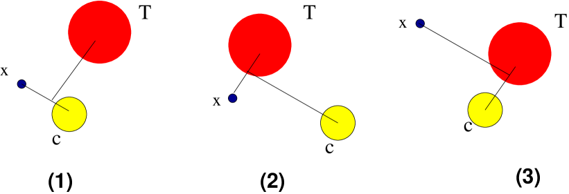
When considering reactions with light radioactive beams, it is customary to model the incoming projectile as a two-body system (in fact sometimes the projectile has a clear three-body structure and models that handle three-body projectiles are underway). In principle, the solution to the reaction problem can be obtained exactly from solving the Faddeev equations with the appropriate boundary conditions. In the Faddeev formalism Fad60 ; Joa87 , the three-body wavefunction is written as a sum of three Jacobi components represented in Fig. 1. Each component is defined by the intercluster coordinate between two of the subsystems ({${\bf r}_{i};i=1,2,3$}) and the relative coordinate of this pair to the third cluster ({${\bf R}_{i};i=1,2,3$}). Asymptotically, the Faddeev component $i$ contains contribution from the bound states associated to the pair with relative coordinate ${\bf r}_{i}$, plus a contribution coming from three-body breakup. Therefore, while rearrangement channels are confined to specific Faddeev components, breakup is distributed among the three components. Consequently, extracting the breakup observables requires complicated transformations among Jacobi coordinates. Besides, solving the Faddeev coupled equations is a very difficult task, specially for three charged particles where Coulomb plays an important role. Inclusion of absorption in the intercluster potentials, which is required when the subsystems have internal degrees of freedom is also an open problem, although some promising work is already in progress akram .

It is well known that basis states belonging to different Jacobi sets are not mutually orthogonal. Furthermore, for each Jacobi set, a complete basis of the three-body bound and unbound spectrum can be constructed. Then, it could be possible, in principle, to describe the reaction observables of a thee-body scattering problem using uniquely states from one of the Jacobi components. This is in fact the procedure followed by the Continuum Discretized Coupled Channels (CDCC) formalism. This method has been applied for more than two decades to the scattering of weakly bound (two-body) projectiles by light and heavy targets. For the scattering of a composite projectile $A$(=$c$+$x$) by a target $T$, the CDCC method defines the model three-body Hamiltonian:

$$H = K_{rel}+H_{int}+U_{x}+U_{c},$$

$$H_{int} = K_{int}+V_{xc}$$ (1)

where $K_{rel}$ is the kinetic energy for the projectile-target relative motion, $K_{int}$ is the internal kinetic energy of the projectile, $U_{x}$ and $U_{c}$ are the $x-T$ and $c-T$ interactions and $V_{xc}$ is the $x-c$ binding potential. As to the internal degrees of freedom of the target, in the standard CDCC method, only the target ground state is considered explicitly. Therefore, the fragments are not allowed to engage in arbitrary processes with the target. For example, processes in which one of the dissociated fragments is absorbed by the target, or in which the target internal degrees of freedom are excited, are excluded from the model space. Also, rearrangement channels corresponding to cluster-target bound states are by construction excluded from the CDCC model space and hence, those observables associated with these two-body channels can not be obtained from the asymptotics of the CDCC three-body wavefunction. The model space spanned by CDCC allows only the calculation of elastic breakup and leaves out those processes related to inelastic breakup.

In order to take into account the effect of the excluded channels, the interactions $U_{x}$ and $U_{c}$ are usually taken as phenomenological optical potentials obtained, for example, from the fit of the elastic data at the same energy per nucleon. By contrast, the interaction $V_{xc}$ is taken to be real, and chosen to reproduce known bound and/or excited states separation energies, or resonance energies.

The full three-body space is truncated by setting a maximum excitation energy for the projectile. Moreover, the $c-x$ relative angular momentum is also restricted by considering only a limited number of partial waves. In order to deal with a finite set of coupled equations, a discretization of the continuum states into energy intervals (bins) is also performed. This procedure should be regarded as a practical method of making the problem numerically solvable, rather than an additional approximation. In fact, it has been shown that the calculated observables are essentially independent of the method of discretization Piy99 .

Within this restricted model space, the three-body wavefunction is expanded in eigenstates of the internal Hamiltonian $H_{int}$ as

$$\Psi_{\bf K}^{(1)}({\bf r}_{1},{\bf R}_{1})=\sum_{\alpha=0}^{N_{1}}\phi_{\alpha}({\bf r}_{1})\chi_{\alpha}({\bf R}_{1}),$$ (2)

where $N_{1}$ is the number of states considered, $\alpha$ represents all angular momentum quantum numbers as well as excitation energies of the projectile, $\phi_{\alpha}({\bf r})$ are the eigenstates of the two-body Hamiltonian $H_{int}$ and $\chi_{\alpha}({\bf R})$ describes the relative motion between the projectile $A=c+x$ and the target $T$. This expansion of the three-body wavefunction is inserted into the Shrödinger equation that, when projected into the considered internal states, provides a set of coupled equations.

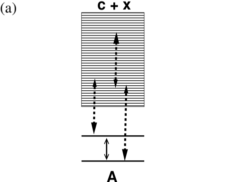
Within the CDCC scheme, the breakup process is treated as inelastic excitations of the projectile $A$ into the continuum $c+x$ due to the interactions with the target $T$ Yah82 ; Yah86 ; Aus87 . A pictorial representation of these couplings is given in Fig. 2(a). The couplings responsible for this excitation, as well as the diagonal potentials, are obtained by folding the phenomenological interactions $U_{x}$ and $U_{c}$ with the internal wavefunctions, i.e.

$$U_{\alpha;\alpha^{\prime}}({\bf R}_{1}) = \langle\phi_{\alpha}|U_{x}+U_{c}|\phi_{\alpha^{\prime}}\rangle\;.$$ (3)

Applications to the breakup of ⁸B at low and intermediate energy regimes have been very successful in describing the data Nun99 ; Tos01 ; Mort02 .

Unlike the Faddeev method, the CDCC approach uses only one of the three possible sets of Jacobi coordinates. As noted above, rearrangement channels corresponding to cluster-target bound states are not part of the CDCC model space and, therefore, the CDCC three-body wavefunction is not adequate to predict observables associated with these two-body channels. On the contrary, it has been argued that, provided that the model space is sufficiently large Aus89 ; Aus96 , the total three-body breakup is contained in the CDCC wavefunction and, hence, can be extracted from its asymptotics.

Although considerably simpler than its Faddeev counterpart, solving the CDCC problem is also a complicated task. In some cases, particularly with heavy targets, long range interactions usually lead to convergence problems. An additional difficulty is that, in many breakup experiments, scattering observables (differential energy cross sections, angular distributions, etc) are obtained with respect to one of the projectile fragments (this is indeed always the case of inclusive reactions). Given the choice of coordinates, the CDCC observables are more naturally expressed in terms of the projectile center of mass, and its internal excitation energy. Converting to one of the fragment’s coordinates requires a complicated kinematic transformation Tos01 . Furthermore, due to the restricted model space, the CDCC description is not expected to be good in the region where channels outside the model space play an important role. Discrepancies in large angle scattering data, observed in early applications of the CDCC method to deuteron and ³He breakup Ise86 , have been attributed to this fact.

A way to circumvent the two latter criticisms is to use the T-matrix formalism in post-form and approximate the incoming exact three-body wavefunction appearing in the exact scattering amplitude:

$$T_{post}=\langle\chi^{(-)}_{cB}\phi^{(-)}_{xT}|V_{xc}+U_{c}-U_{f}|\Psi_{i}^{(+)}\rangle,$$ (4)

by the CDCC wavefunction, i.e., $\Psi_{i}^{(+)}\approx\Psi^{CDCC}$. In this equation, $B=x+T$, $\chi^{(-)}_{cB}$ is the distorted wave generated by the (arbitrary) distorting potential $U_{f}(\mathbf{R^{\prime}})$ (where $\mathbf{R^{\prime}}$ is the $c-B$ relative coordinate), and $\phi^{(-)}_{xT}$ represents a scattering state for the $x+T$ system. By making use of the Gell-Mann–Goldberger two-potential formula, the transition amplitude (4) can be rewritten as:

$$T_{post}=\langle\chi^{(-)}_{cT}\phi^{(-)}_{xT}|V_{xc}|\Psi_{i}^{(+)}\rangle,$$ (5)

where $\chi^{(-)}_{cT}$ is the distorted wave generated by the potential $U_{c}$. The above matrix element is dominated by small $x-c$ separations, where $\Psi^{CDCC}$ is at its best.

Although very appealing from the formal point of view, expression (5) is hard to implement in practice. The main reason is that this expression involves a six-dimensional integral, in which both the initial and final wavefunctions are highly oscillatory. Furthermore, post form representations offer poor convergence since both the scattering waves for $x+c$ and the potential $V_{xc}$ are expressed in the same coordinate and consequently there maybe no natural cutoff for the integral (5) Ich85 .

In order to make the calculation more feasible, Shyam and collaborators (see, for instance, Ban98 ; Chat00 ; Chat02 ) have developed an approach based in the amplitude (5), in which the exact wavefunction is replaced by its elastic component, i.e.,

$$\Psi_{i}^{(+)}\approx\chi_{0}^{(+)}(\mathbf{R}_{AT})\phi_{0}(\mathbf{r}_{xc}),$$ (6)

where $\phi_{a}(\mathbf{r}_{xc})$ is the projectile ground state and $\chi_{0}^{(+)}$ is a distorted wave generated with a optical potential, typically adjusted to reproduce the elastic scattering data. Note that this approximation neglects breakup events that proceed via projectile excitation. Note also that, even after the replacement of the exact wavefunction by the elastic component, Eq. (5) still involves a six dimensional integral. A significant simplification of the problem can be achieved by using the local momentum approximation Shy85 ; Chat00 , which leads to a factorization of the amplitude in a product of two terms, each involving a three-dimensional integral.

Figure 2: : (a) Breakup couplings for a two-body projectile ($c+x$) impinging on a target $T$ and (b) corresponding transfer to the continuum couplings.

The difficulties outlined above can be partially avoided using the prior representation of the transition amplitude,

$$T_{prior}=\langle\Psi_{f}^{(-)}|V_{xT}+U_{c}-U_{AT}|\phi_{0}\chi_{0}\rangle,$$ (7)

where the final state is the exact three-body wavefunction with incoming boundary conditions. This wavefunction is typically expanded in terms of the $x+T$ continuum states, formally similar to Eq. (2), but now in the Jacobi set (2) of Fig. 1:

$$\Psi_{f}^{(2)}({\bf r}_{2},{\bf R}_{2})=\sum_{\beta=0}^{N_{2}}\phi_{\beta}({\bf r}_{2})\chi_{\beta}({\bf R}_{2}).$$ (8)

Again, the functions $\phi_{\beta}$ represent the set of bin wavefunctions Yah82 ; Yah86 ; Aus87 , constructed by superposition of pure scattering waves. Note that Eq. (8) goes beyond the DWBA, because couplings between final states are explicitly considered in the wavefunction $\Psi_{f}^{(2)}$.

Therefore, in the standard CDCC method the three-body continuum is described in terms of the projectile two-body ($x-c$) states, while in the amplitude (7) this continuum is expanded using the fragment-target states $x-T$. While the CDCC method treats the breakup process as inelastic excitations to the projectile continuum, expressions (5) and (7) emphasize a rather different picture, in which three-body breakup is formally treated as transfer of one of the fragments ($x$ in our case) to the target continuum. This is schematically illustrated in Fig. 2(b). At this stage, it is worth to stress that, in the way here presented, the CDCC and the the TR* methods are solutions of the same three three-body model Hamiltonian, given by Eq. (1) and, therefore, three-body observables obtained with these two approaches should be the same.

However, in practice there are several factors that may destroy this equivalence. First, due to computational limitations, one can not include an arbitrarily large number of continuum states. Secondly, there are ambiguities associated with the choice of the interactions involved in both schemes. In the BU approach, one usually has two complex potentials, namely $U_{x}$ and $U_{c}$, and a real interaction, $V_{xc}$. By contrast, in the amplitude (7) the wavefunction $\Psi_{f}^{(2)}$ is typically obtained with the complex potentials $U_{c}$ and $U_{xc}$. The choice of the potential $V_{xT}$ deserves special care. For inclusive processes, in which the fragment $x$ is allowed to interact in any possible way with the target, $V_{xT}$ would be a complicated many body operator, which can induce excitations in both $x$ and $T$. However, for a comparison with CDCC, in which only the elastic breakup component is calculated, this operator is better represented by an effective complex optical potential Ich85 ; Aus87 and hence, according to our previous notation, $V_{xT}=U_{x}$. This is actually the choice made in current semiclassical applications of the transfer to the continuum method Bon01 .

Another ambiguity is related to the interaction that should be used for $U_{AT}$ in the amplitude (7). Note that, if the exact expression is used for the three-body wavefunction $\Psi_{f}^{(-)}$ the matrix element is independent of the choice of the potential $U_{AT}$. This result does not hold when $\Psi_{f}^{(-)}$ is replaced by an approximated wavefunction. Following the standard DWBA choice, one could use the optical potential that reproduces the elastic scattering. Another possible choice, is the so called cluster-folding potential, given by the sum of the fragments-target interactions folded with the ground state of the projectile: $\langle\phi_{0}|U_{x}+U_{c}|\phi_{0}\rangle$. In our calculations we have explored both choices.

The main purpose of this work is to test to what extent the equivalence between the BU and (prior form) TR* is satisfied, at least in an approximate way, in actual calculations. To this end, we have performed numerical calculations for two different systems using both approaches, and compared several reaction observables. At high scattering energies, around 100 MeV per nucleon and above, the TR* method, as presented here, becomes numerically very demanding, and the problem is better solved by using further approximations, such as the use of classical trajectories. Since it is our purpose to compare the full quantum mechanical CDCC and TR* expressions, we confine ourselves to reactions at low and medium energies.

III Calculations

III.1 $p$+¹¹Be case

We first consider the reaction of 38.5 MeV per nucleon ¹¹Be breaking up on protons. The elastic and transfer channels were measured in GANIL Win01 ; lapoux but no breakup data was recorded. According to the discussion in the previous section, the ¹¹Be breakup reaction can be thought of as the direct breakup (BU) ¹¹Be$+p\rightarrow(^{10}$Be$+n)+p$ or transfer of the neutron to the continuum of the deuteron (TR*) ¹¹Be$+p\rightarrow^{10}$Be$+(n+p)$.

The $n-p$ interaction was taken from Aus87 , whereas the nuclear interaction for $p-^{10}$Be was extracted from a fit to the elastic data lapoux . The Coulomb potential for $p-^{10}$Be was also included so Coulomb breakup is also included in our calculations, although it was shown to be very small. The binding potential and the potential generating the continuum waves for $n-^{10}$Be was the same as in Win01 , but without the spin-orbit term. These potentials are listed in Table 1. The BU calculations required partial waves up to $l_{max}=4$ and energies up to $\varepsilon_{max}$=30 MeV for the relative motion of the $n-^{10}$Be system. The bin wavefunctions for the CDCC couplings were calculated up to $R_{bin}$=60 fm. An $L_{max}=25$ was necessary for the ¹¹Be$-p$ distorted waves. As to the TR* calculation, the same parameters were sufficient for convergence but they are computationally more lengthy . All the TR* calculations here presented use as incoming optical potential the folding of the $p-n$ and $p$-¹⁰Be interactions with the ground state wavefunction of the ¹¹Be nucleus. We also did calculations using a Woods-Saxon shape with the same parameters as for the $p$-¹⁰Be potential. Results obtained with this potential are very similar to those of the cluster-folding and, hence, will not be shown in the graphs. Both the BU and TR* calculations were performed with the computer code FRESCO Thom88 .

Table 1: Optical model parameters used in this work. Except for the $p+n$ case, all potentials are parameterized using the usual Woods-Saxon form, with a real volume part and volume ($W_{v}$) or surface ($W_{d}$) imaginary part. Reduced radii are related to physical radii by $R=r_{0}A_{T}^{1/3}$.

System	$V_{0}$	$r_{0}$	$a_{0}$	$W_{v}$	$W_{d}$	$r_{i}$	$a_{i}$
	(MeV)	(fm)	(fm)	(MeV)	(MeV)	(fm)	(fm)
$p$+10Be	51.2	1.114	0.57	19.5	0	1.114	0.50
$p+n$	72.15	1.484	-	-	-	-	-
8B+58Ni	130	1.050	0.65	92	0	1.123	0.997
7Be+58Ni	100	1.050	0.65	30.6	0	1.123	0.80
$p$+58Ni	54.512	1.17	0.75	0	11.836	1.260	0.58
$p$+7Be	44.675	1.25	0.52	-	-	-	-

Figure 3: (Color online) Breakup energy distribution for ¹¹Be on protons at 38.5 MeV/u: comparison of transfer to the continuum (bottom figure) with the direct breakup approach (upper figure).

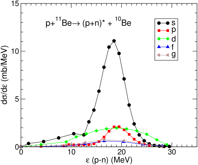
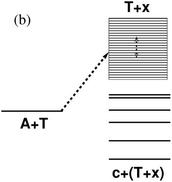
In Fig. 3 we present the differential breakup cross section calculated within the BU and TR* methods, as a function of the excitation energy of the ¹⁰Be-$n$ and $p$-$n$ systems, respectively. It can be seen that, in the BU case, most of the strength is below $\varepsilon_{x}(^{11}$Be$)\approx 5$ MeV whereas in the TR* calculation the strength is largely concentrated around $\varepsilon_{x}(d)\approx 20$ MeV. The total integrated cross section for the two processes are $\sigma_{bu}=125$ mb and $\sigma_{tr}=140$ mb.

Figure 4: Total angular momentum distribution for the breakup of ¹¹Be on protons at 38.5 MeV/u: comparison of transfer to the continuum with the direct breakup approach.

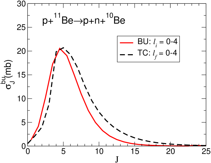
In order to establish a meaningful comparison between the two approaches, one has to compare the same quantities. For this purpose, in Fig. 4 we compare the contribution of each total angular momentum $J$ (resulting from the vector coupling of projectile, target and their relative motion angular momentum) to the breakup cross section. It can be seen that both distributions are similar for small values of $J$. Also, we find that for the two cases the distribution peaks around $J=5$ which means that most of the breakup cross section occurs at distances $b\approx 4$ fm. The similitude between both distributions supports the idea that breakup, calculated as excitation of the projectile to its continuum spectrum, or by transfer to the continuum states of the target, do describe the same physical process. However, for $J>5$ the TR* clearly exceeds the BU cross section which, as we will show below, results on different predictions for measurable physical observables.

In actual breakup experiments, the data commonly recorded are the angular and/or energy distributions of the emerging fragments. Therefore, it is instructive to compare the predictions of both approaches for these observables. In Fig. 5 we represent the calculated breakup cross section distribution of the outgoing ¹⁰Be fragments as a function of its kinetic energy, measured in the overall c.m.  of the three-body system. In both methods, these distributions are obtained by integration of a triple differential cross section with respect to the angular variables. In the case of the TR* approach, this procedure is straightforward, since expression (7) is referred already to the scattering angle and energy of the ¹⁰Be fragments. In the case of the BU approach, the differential cross section is naturally expressed in terms of the scattering angle of the composite $x+c$ and the relative energy between these two fragments. In order to obtain the differential cross section with respect to any of the fragments, one has to apply to appropriate kinematic transformation, as done in Ref. Tos01 .

Figure 5: Energy distribution in the overall c.m. for the ¹⁰Be coming from the breakup of ¹¹Be on protons at 38.5 MeV/u: comparison of transfer to the continuum with the direct breakup approach.

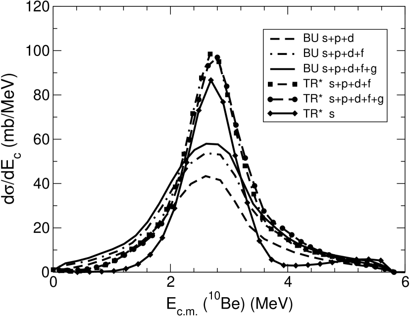
These energy distributions show only a qualitative agreement between the two methods. In both cases, the energy of the ¹⁰Be fragments goes from zero to about 6 MeV, with a maximum around 3 MeV. However, although the same energy region of space is being included, the two models do not produce identical shapes. In Fig. 5 we also show the convergence rates for both TR* and BU. The labels s,p,d, etc refer to the relative partial waves included in the corresponding calculation. For instance, the solid line in the BU calculation includes all $n-^{10}$Be partial waves up to $l=4$ whereas the dashed line includes only partial waves up to $l=2$.

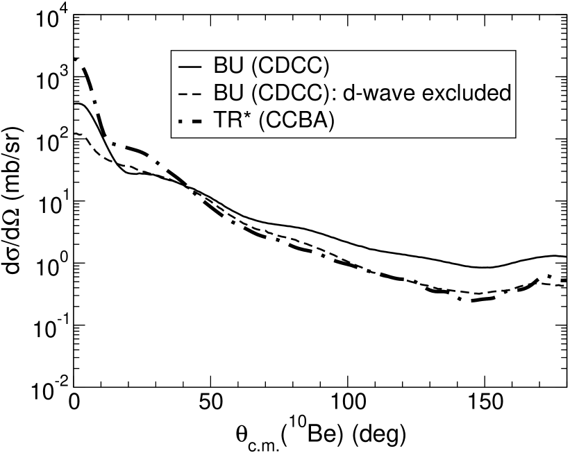
Disagreements become more severe for the angular distributions. These can be seen in Fig. 6. Note that the TR* calculation (dot-dashed curve in Fig. 6) exhibits a pronounced decrease of the cross section as a function of angle. In addition, its forward angle cross section is an order of magnitude larger than the BU calculation (solid line) and an order of magnitude lower for backward angles. Part of the reason for the disagreement can be understood excluding the d-wave resonance in the $n-^{10}$Be system (dashed curve). This wave has a very strong contribution for backward angles and a d-wave resonance in ¹¹Be will be very hard to model in terms of the deuteron continuum. However, the discrepancy remains at forward angles: including only the s-wave of the deuteron in the BU calculation, the resulting cross section is an order of magnitude smaller than the TR* cross section. Detailed data for this reaction would be very useful.

Figure 6: Angular distribution in the c.m. for the ¹⁰Be coming from the breakup of ¹¹Be on protons at 38.5 MeV/u: comparison of transfer to the continuum with the direct breakup approach.

III.2 ⁸B+⁵⁸Ni case

A breakup reaction for which more detailed data exist is that for ⁸B$\rightarrow^{7}$Be$+p$ on ⁵⁸Ni at 25.6 MeV. Calculations using the standard CDCC ⁸B$+^{58}$Ni $\rightarrow(^{7}$Be$+p)+^{58}$Ni have provided very good agreement with experiment Nun99 ; Tos01 . Again, one can think of the alternative path to breakup, as transfer to the continuum of the ⁵⁹Cu nucleus (TR*) ⁸B$+^{58}$Ni $\rightarrow^{7}$Be$+(p+^{58}$Ni). All interactions for both BU and TR* are the same as those in Tos01 , although for the $p-$Ni only the real part was included in the TR* calculation.

The BU calculations required partial waves up to $l_{max}=4$ and energies up to $\varepsilon_{max}=8$ MeV for the relative motion of the $p$-⁷Be system. The bin wavefunctions for the CDCC couplings were calculated up to $R_{bin}=60$ fm and the coupled channel equations were solved with $R_{max}=500$ fm. An $L_{max}=1000$ was necessary for the ⁸B$-^{58}$Ni distorted waves . Note that in this case the BU calculation is a good test reference, as it agrees very well with both energy and angular distribution data Tos01 , at least within the kinematic conditions of the referred experiment. As to the TR* calculation we used partial waves up to $l_{max}=17$ and energies up to $\varepsilon_{max}=10$ MeV for the relative motion $p+^{58}$Ni. To reduce the computational requirements, for $l_{f}>6$, continuum–continuum couplings were included only between bins with the same $l_{f}$. The bin wavefunctions were calculated up to $R_{bin}=120$ fm, and an $L_{max}=120$ was necessary for the ⁸B$-^{58}$Ni distorted waves. However, these results are not yet converged. The large required widths for the non-local transfer couplings make the calculations extremely heavy.

We next compare the same quantities as in the $p$+¹¹Be case. Unlike the previous test example, where $V_{xc}=V_{pn}$, here the $V_{xc}$ interaction ($p$+⁷Be), as extracted from the elastic data, is expected to contain an imaginary part. In our TR* calculations, we probe several possibilities for the imaginary part, keeping the same geometry as the real part and using different choices for the depth. For the incoming channel optical potential we used two different potentials. The first one, denoted OM1, is the sum of the $p$+⁷Be and ⁷Be+⁵⁸Ni interactions folded with the bound state wavefunction of the ⁸B nucleus. The second one, consisted on a parametrization with two Woods-Saxon terms, real and imaginary, with parameters obtained by fitting the elastic angular distribution, as predicted by the CDCC calculation. In this case we used, as starting parameters for the fitting routine, those for the ⁷Be+⁵⁸Ni interaction. The parameters for this potential resulting from the fit, denoted OM2, are listed in Table 1.

Figure 7: Total angular momentum distribution for the breakup of ⁸Be on ⁵⁸Ni at 25.6 MeV. The solid line is the BU calculation, whereas the remaining lines correspond to the TR* calculations with two different sets of partial waves $l_{f}$, as indicated by the labels (see text for details).

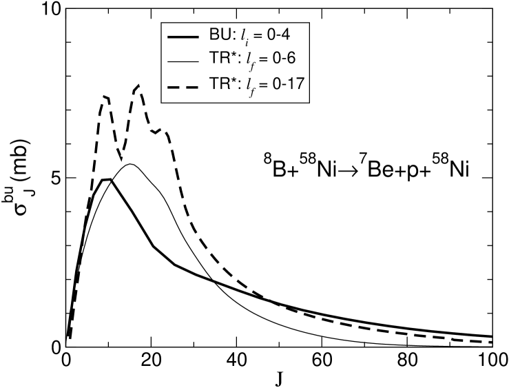
In Fig. 7 we show the total breakup calculated within the BU and TR* schemes, for each value of the total angular momentum, $J$. In the TR* case, two different calculations are presented. In both cases, the potential OM2 was used for the elastic channel, and the value $W_{d}$=3 was used for the imaginary depth of the $p$+⁷Be interaction. The thin solid line in this figure represents the TR* calculation performed in the subspace $l_{f}=0-6$. This calculation exhibits clear differences from the BU (thick solid line): the lower values of $J$ are clearly overestimated, whereas for the large values of $J$, the distribution falls too fast as compared to the BU. The second TR* calculation here presented (dotted-dashed line) uses the same parameters as before, but includes also the partial waves $l_{f}=7-17$ for the proton-⁵⁸Ni continuum. This calculation improves the agreement for large $J$. However, it also adds an extra contribution on the lower values of $J$ which appears to deteriorate the agreement with the BU results.

As noted in the previous section, it has been argued that in the calculation of elastic breakup, one should use an absorptive potential for the $V_{xT}$ operator in Eq. (7). This might explain part of the discrepancies found here between both approaches. Unfortunately, the present version of the code FRESCO does not allow this interaction to be complex. Although at present we cannot use an imaginary term in the $V_{xT}$ operator, we are considering modifications of the code to enable this feature. It is fortunate that, in the $p$+¹¹Be reaction, $V_{xT}=V_{pn}$ which, within the energy range of our analysis, is well represented by a real potential. This might explain the better agreement obtained for the absolute value of the breakup cross section, as well a for the $J$-distribution, as compared to the ⁸B+⁵⁸Ni case.

Although the representation of the $V_{xT}$ operator by a real operator has undesirable consequences for the purpose of the present work, one may speculate about the physical meaning behind this choice. As noted above, choosing $V_{xT}$ as the phenomenological optical potential in the CDCC approach implies that the model space considers only breakup where the target is left in its ground state. Conversely, one may argue that, by choosing this potential as real, as we do here in the TR* case, there is the possibility of including other inelastic breakup events, and even transfer to bound states of the target. In other words, the TR* method with a real $V_{xT}$ may include contributions from the so called stripping breakup. These aspects will be explored in future work.

Figure 8: (Color online) Angular distribution in the laboratory frame for the ⁷Be fragments coming from the breakup of ⁸B on ⁵⁸Ni at 25.6 MeV within the direct breakup and transfer to the continuum approaches. Experimental data are from Gui00 .

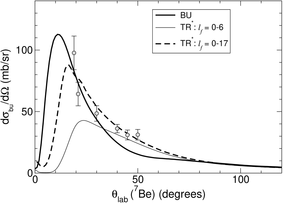
For the ⁷Be angular distribution, we first study the convergence of the calculations with respect to the size of the model space. In the case of the BU this has been discussed in detail in Ref. Tos01 , and so we will just quote the results from this reference. In this section, we concentrate only on the convergence of this observable within the TR* scheme. For definiteness, these calculations were performed with the choice $W_{d}=3$ MeV for the imaginary part of the $p$+⁷Be potential. The dependence on this potential will be analyzed below. The convergence of the calculation with respect to the number of partial waves for the relative motion of the $x-T$ pair is depicted in Fig. 8. For comparison, the BU calculation (thick solid line) and the experimental data points Gui00 have been also included. The thin solid line is the calculation where the partial waves $l_{f}=0-6$ are included and coupled among them to all orders. The thick dotted-dashed line is the sum of this calculation and the separated differential cross sections for the partial waves $l_{f}=7-17$. It becomes apparent that the contribution of these partial waves is very important to describe the strong Coulomb peak at small scattering angles. Both calculations are in good agreement with the data. Given the large error bars and restricted angular range of the data it is not possible to make strong conclusions on which method is more suitable in this particular situation. Roughly speaking, it seems that the TR* describes better the larger angles, while the BU is more suitable to describe the smaller angles. In the remaining discussion, all our comparisons with the BU calculations will be performed with the full set of partial waves ($l_{f}=0-17$).

Figure 9: Angular distribution in the c.m. for the ⁷Be fragment coming from the breakup of ⁸B on ⁵⁸Ni at 25.6 MeV: comparison of transfer to the continuum with the direct breakup approach for two different choices of the incoming optical potential for the TR* calculation (see text for details).

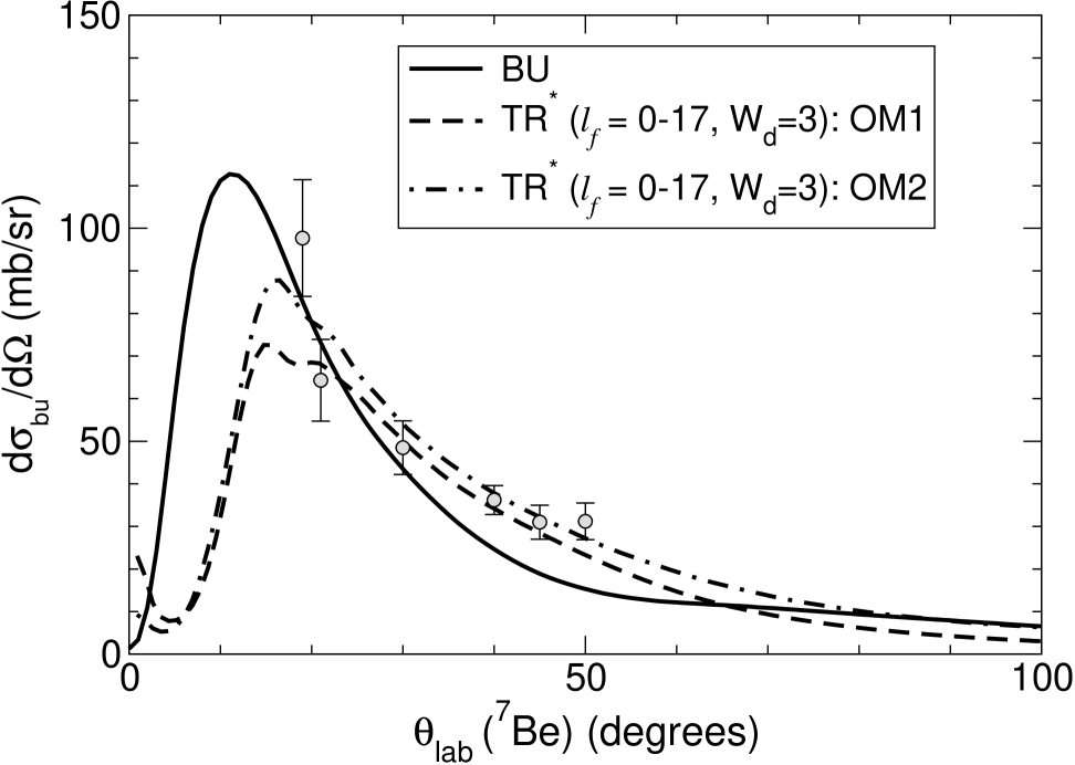
Next, we study the dependence of the ⁷Be angular distribution on the choice of the incoming channel optical potential. This is illustrated in Fig. 9. In this figure, the dashed and dotted-dashed lines correspond, respectively, to the TR* calculation with the cluster-folded potential (OM1) and the phenomenological optical potential obtained from a fit of the CDCC elastic angular distribution (OM2). Again, we have fixed the imaginary depth of the $p$+⁷Be interaction to $W_{d}=3$ MeV. For comparison purposes, the BU calculation (thick solid line) has been also included. One sees that the choice of the elastic channel optical potential has indeed an effect on the predicted ⁷Be cross sections. However, given the uncertainties of these calculations, differences do not seem very dramatic, and in both cases a fairly good agreement is obtained with the BU calculation irrespective of the choice of this potential.

Figure 10: (Color online) Angular distribution for the ⁷Be fragments coming from the breakup of ⁸B on ⁵⁸Ni at 25.6 MeV: comparison of transfer to the continuum with the direct breakup approach for different values of the imaginary depth of the $p$+⁷Be potential.

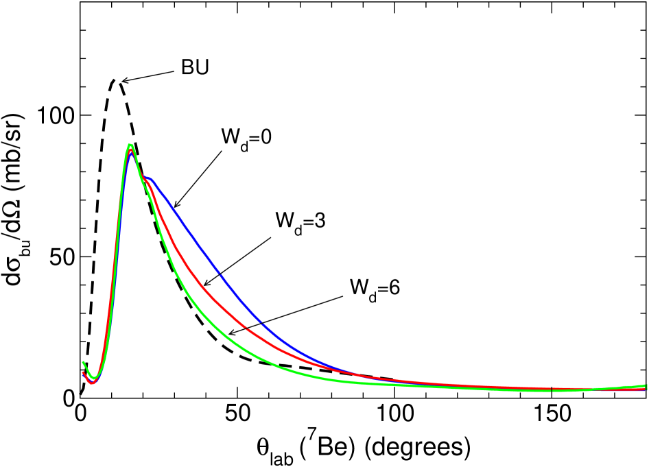
In Fig. 10 we compare the standard CDCC calculation with TR* calculations performed with the optical potential OM2 for the incoming channel, and different choices of the imaginary depth of the $p$+⁷Be potential. Thick lines correspond to the full calculation ($l_{max}=17$). At backward angles all TR* calculations look very similar, indicating a fast convergence with respect to the number of partial waves and a weak dependence on the choice of the $p$+⁷Be potential at these angles. The effect of the imaginary part seems to be crucial at intermediate angles, where one observes a progressive suppression of the cross section with increasing absorption. The TR* with real $p$+⁷Be interaction clearly overestimates the BU result at intermediate angles. Interestingly, the forward angular region is only weakly affected by this absorptive term. As we verified in our calculations, this is a consequence of the fact that this potential has little effect on the higher partial waves. The best agreement with the BU calculation is obtained when the imaginary part of the $p$+⁷Be potential for TR* is $W_{d}=6$ MeV.

The reasonably good agreement between BU calculation and the TR* calculations, performed in the augmented model space ($l_{max}=17$) and with a complex proton+⁷Be interaction, leads us again to the conclusion that projectile breakup and transfer to the target continuum populate, to a large extent, the same three-body continuum. We interpret the discrepancy at small scattering angles as lack of convergence of our TR* calculations, and the ambiguities associated to the potentials.

Figure 11: Energy distribution in the c.m. for the ⁷Be coming from the breakup of ⁸B on ⁵⁸Ni at 25.6 MeV: comparison of transfer to the continuum with the direct breakup approach.

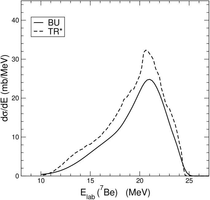
In Fig. 11, we plot the energy distribution for the detected ⁷Be fragments after breakup, for the BU (solid line) and the TR* approach with $l_{max}=17$, and $W_{d}=3$ MeV for $p$+⁷Be (dashed line). It can be seen that both methods give similar distributions. In particular, it is noticeable that both methods predict a maximum of the energy distribution at about the same ⁷Be energy. The TR* calculation gives however a larger breakup cross section.

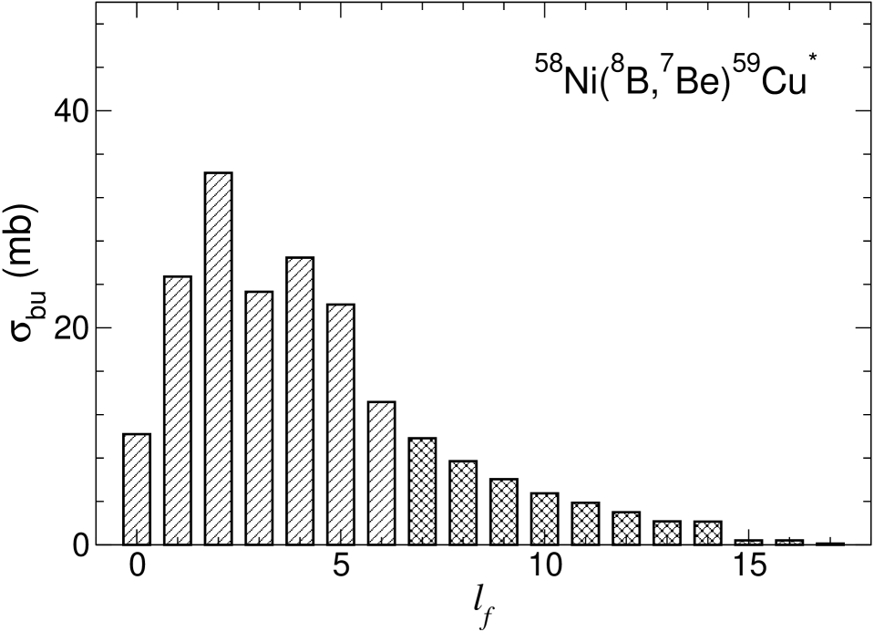
To have further insight into the convergence of the TR* calculation with respect to the size of the model space we have plotted in Fig. 12 the distribution of the TR* cross section as a function of $l_{f}$, i.e., the final angular momentum between the proton and the target. On one hand, it is clear that TR* requires far more partial waves that the BU calculation. On the other hand, the small contribution for $l_{f}>15$, does provide some confidence in the results presented here.

Figure 12: Breakup distribution as a function of the relative motion ⁵⁸Ni-p for the transfer to the continuum of the proton from ⁸B to ⁵⁸Ni at 25.6 MeV. Results up to $l_{f}=6$ are fully coupled, but for $l_{f}>6$ they are calculated separately (see text for details).

The breakup of ⁸B on ⁵⁸Ni at 25.8 MeV is a good example where the BU configuration seems to work better than the TR* configuration.

IV Discussion

The qualitative agreement between the calculations performed in the BU and TC representations clearly indicates that both basis describe to a large extent the same three-body continuum. However, the analysis of the preceding section also shows that, in order to achieve convergence of the observables, the number of basis states required in both representations can be very different. From the practical point of view, it will be desirable in general to choose the representation that requires less number of states.

For example, our analysis of the ⁸B breakup reaction clearly supports the choice of the Jacobi coordinates (1) in Fig 1. On the other side, our previous study on the reaction ⁸Li+²⁰⁸Pb Mor03a was better performed using the coordinate set (2). It is clear that, in general, the most suitable choice will depend on the specific reaction. Inspired by the work of Merkuriev Merk74 on three-body bound states, we have searched for a criterion that can select between the two representations. Unfortunately the asymptotic behaviour of the three body continuum is very different from the exponential decay of bound states, and the final behaviour of these expansions is not as transparent. Therefore, we will present only qualitative arguments to evaluate the relative importance of the different configurations.

For practical purposes one always opts for the calculation that requires the minimum number of partial waves in the $x-c$ or $x-T$ systems, for BU and TR* respectively. For the ¹¹Be the difference in $l_{max}$ for BU and TR* was not noticeable. For the ⁸B example, $l_{max}=4$ was sufficient for BU whereas $l_{max}=17$ was still not enough for the TR*. In addition to the angular momentum, it seems clear that if a representation such as Eq. (2) is valid, then the average energy $\langle\varepsilon_{1}\rangle$ associated with the relative coordinate $r_{1}$ should be much less than the total energy in the centre of mass frame $E_{cm}^{(1)}$. Equally, if Eq. (8) is to be used, the average energy $\langle\varepsilon_{2}\rangle$ associated with coordinate $r_{2}$ should be small compared to the total energy of the exit partition in the centre of mass frame $E_{cm}^{(2)}$. We have computed the average energy between the fragments in the continuum, weighting it by the cross section. For the ⁸B example above, we obtain $\langle\varepsilon_{1}\rangle=1.85$ MeV with $E_{cm}^{(1)}=22.7$ MeV for the BU calculation and $\langle\varepsilon_{2}\rangle=7.84$ MeV with $E_{cm}^{(2)}=26.0$ MeV for the TR* calculation. In the first case $\langle\varepsilon_{1}\rangle/E^{(1)}_{cm}=0.08$ whereas in the latter $\langle\varepsilon_{2}\rangle/E^{(2)}_{cm}=0.30$. As to the ¹¹Be example, the difference is also pronounced: for BU we obtain $\langle\varepsilon_{1}\rangle/E^{(1)}_{cm}=0.15$ and $\langle\varepsilon_{2}\rangle/E^{(2)}_{cm}=0.52$, implying again that the transfer to the continuum approach is not the best. In the breakup of ⁸Li Mor03a , the TR* approach was used successfully. We compute the average energy between the fragments in the outgoing channel and obtain $\langle\varepsilon_{2}\rangle/E^{(2)}_{cm}=0.05$, validating the previous TR* calculations Mor03a . This same criterion shows a red card to the preliminary calculations on ⁶He Agu00 , as in that case we have $\langle\varepsilon_{2}\rangle/E^{(2)}_{cm}=0.43$. In conclusion, the condition $\langle\varepsilon^{i}\rangle/E^{i}_{cm}\ll 1$ should be satisfied whenever only one $i$ Jacobi set is taken into account in the reaction formalism. This is for instance the case in Coulomb dissociation, where the long-range and smooth behaviour of the Coulomb potential makes that the reaction mechanism populates mainly low-energy states of the projectile. As a matter of fact, is was shown in Nun99 that the peak in the breakup angular distribution at $\theta_{\mathrm{c.m.}}\approx 15^{\circ}$ is mainly due to Coulomb excitation. In our calculations, this peak is well reproduced by the CDCC calculation, while it requires many partial waves of the proton-target system in the TR* method. Furthermore, at high energies, the Coulomb dissociation cross section becomes approximately proportional to the $B(E1)$ strength of the projectile. Hence, the BU approach provides in this case a more transparent and useful picture of the reaction process. On the other side, in situations where the removed particle has a high probability to be left with a small relative energy with respect to the target, the TR* may result more convenient. Nevertheless, this does not seem to be the case of the reactions studied in this work.

Even in calculations where the TR* converges quickly with the number of partial waves, we found it to be computationally very demanding, as it involves non-local couplings. In practice, these calculations could be significantly speeded up, using different techniques which are now of common use: local momentum and adiabatic approximations, etc. It is however beyond the scope of this work to explore how to make the TR* numerically more feasible.

V Conclusions

Given the importance of the reaction model in the understanding of the fundamental nuclear structure on the drip lines, we compare two alternative schemes to calculate breakup observables for the reaction $A(=c+v)+T$, within the same three-body Hamiltonian. Each one of these methods uses a description of the three-body continuum in terms of one of the possible sets of Jacobi coordinates. In the CDCC approach, the three-body continuum is described in terms of the $c-v$ states. On the contrary, the transfer to the continuum (TR*) approach expands the continuum in terms of $v-T$ states. Since both sets of states form a complete basis, reaction observables could be in principle calculated using either of these two basis. We show that in both cases predictions by these two schemes are in semiquantitative agreement. This result clearly shows that, provided that enough basis states are included, both representations describe essentially the same three-body continuum. In the ⁸B+⁵⁸Ni reaction, both calculations are consistent with existing experimental data. From our analysis, it is clear that the truncated model space is not always identical. In particular, in this case we found that the TR* approach requires a significantly larger number of partial waves for the proton-cluster relative motion, thus making the calculation numerically more demanding. We also find that part of the disagreement between the two methods is due to the ambiguities associated with the choice of the effective interactions involved in both methods. In addition, we have proposed a simple criterion based on the average relative excitation energy to select between the two approaches.

More detailed studies on the absorption part of the optical potential and applications to other reactions will be presented elsewhere. Ultimately, we would like to compare these results with exact Faddeev calculations. Work along these line is being initiated.