Isospin fluctuations in spinodal decomposition

Abstract

We study the isospin dynamics in fragment formation within the framework of an analytical model based on the spinodal decomposition scenario. We calculate the probability to obtain fragments with given charge and neutron number, focussing on the derivation of the width of the isotopic distributions. Within our approach this is determined by the dispersion of $N/Z$ among the leading unstable modes, due to the competition between Coulomb and symmetry energy effects, and by isovector-like fluctuations present in the matter that undergoes the spinodal decomposition. Hence the widths exhibit a clear dependence on the properties of the Equation of State. By comparing two systems with different values of the charge asymmetry we find that the isotopic distributions reproduce an isoscaling relationship.

I Introduction

In the last years a widespread attention has been devoted to the role played by the isospin degree of freedom in the heavy–ion reaction physics. The interest on this subject is twofold: the knowledge of the symmetry term in the Equation of State (EOS) of asymmetric nuclear matter, which is a fundamental ingredient in astrophysical investigations Lat01 , and the thermostatistical properties both at equilibrium and out of equilibrium of systems with two strongly interacting components Mue95 ; Bao97 ; Bar98 ; Lar99 ; Bot01 ; Bar01 ; Bar02 . Both the interests concern systems faraway from the physical conditions of ordinary nuclear matter.

Thanks to the availability of high–performance $4\pi$–detectors for the investigations of heavy–ion collisions at intermediate energy Xu00 ; Tsa01 ; Xu02 ; Ger04 , recent experimental results can provide new insights about isospin effects on the nuclear dynamics. In particular, for multifragmentation processes we can obtain information about highly excited two–component systems and their subsequent decomposition. Statistical models have been extensively applied to the description of experimental data, also for isospin observables Tan03 , and some conclusions have been drawn on the behavior of charge asymmetric systems. These models, however, imply the achievement of the statistical equilibrium for the nuclear system. Then, it would be highly desireable to have some insight on the path followed by the system to attain equilibrium, if this occurs. Further, it would be of great advantage to envisage some observable, which preserves memory of the dynamical processes occurred during the fragmentation.

In this paper we present an analytical description of the disassembly of excited nuclear systems formed during the collision of heavy ions, in terms of the occurrence of nuclear matter instabilities. Our approach accounts for the source of the density fluctuations occurring when the system enters the spinodal instability region of the density–temperature phase diagram, and describes the growth of the fluctuations with time until they cause the decomposition of the system. This approach is a generalization to include the isospin degree of freedom, of the model developed in Refs. Mat00 ; Mat03 for symmetric nuclear matter basically. This gives rise to a substantial improvement of the model, with new valuable results. Such extension allows us to investigate separately fluctuations of the neutron and proton densities and their interplay. Following the procedure introduced in Ref. Mat00 , we identify the pattern of the domains containing correlated density fluctuations, with the fragmentation pattern, and can make predictions on the isotopic distributions of the fragments. Moreover, we include in the present treatment the Coulomb force according to the approach outlined in Ref. Fab98 . Its effects on the isotopic distributions turn out to be sizeable.

Our results essentially refer to the distributions of the fragments just after the early break–up of the system. So our approach can be considered complementary to dynamical model calculations based upon semiclassical kinetic equations for one–body phase–space density, (for a review on dynamical models see, e.g., Refs. Das01 ; Bor02 ; Cho04 ), as far as the description of the early fragmentation mechanism is concerned. The advantage here is that one can make significant predictions on observables of experimental interest on an analytical basis. This allows us to directly relate the results obtained to the EOS properties and the features of the spinodal mechanism. In our scheme the onset and the growth of the fluctuations about the mean phase–space density in unstable situations, are self–consinstently treated. The self–consistency condition is provided by the fluctuation–dissipation theorem. Whereas all the processes, which take place before the system enters the spinodal instability region and after the break–up, are beyond our approach. Therefore the mean values of density, temperature and asymmetry of the nuclear medium when the system starts to break up are taken from calculations performed within dynamical models.

On the other side, a dynamical model, which appropriately incorporates the effects of the fluctuations, might give a detailed description of the whole history of a collision between heavy ions. Therefore, it can be of interest to compare the results of our approach with those obtained by numerical solutions of microscopic transport equations, also to connect the results of the simulations to what is expected in a pure spinodal decomposition scenario. The comparison will be done with the isotopic distributions for the primary fragments, calculated in the dynamical stochastic mean–field (SMF) approach of Refs. Bar02 ; Col98 . In particular, we will consider the ratio, for a given value of the proton number, between the isotope yields from two different reactions. This quantity represents a straightforward mean to compare isotopic distributions, since it is experimentally found to obey a simple relationship (isoscaling), as a function of the proton number and neutron number Xu00 ; Tsa01 ; Tan01 ; Tsa101 . We will also discuss the dependence of the isoscaling parameters on the EOS considered.

In Sec. II we outline the extension of the formalism developed in Ref. Mat00 only for isoscalar density fluctuations, to include the isospin degree of freedom. In Sec. III we discuss the results of our calculations and their comparison with the calculations performed in Ref. Liu04 within the SMF approach. Finally, in Sec. IV a brief summary and conclusions are given.

II Formalism

II.1 Time evolution of density fluctuations

We study the density fluctuations by introducing a self–consistent stochastic field acting on the constituents of the system. The time evolution of the fluctuations is described by a kinetic equation, within a linear approximation for the stochastic field. The growth of fluctuations is essentially dominated by the unstable mean field. Thus we focus our attention on the behavior of the mean field and neglect the collision term in the kinetic equation. Collisions would mainly add a damping to the growth rate of the fluctuations and should not change the main results of our calculations, at least at a qualitative level.

The additional stochastic mean field, which we assume having a vanishing mean, will induce fluctuations of the proton and neutron densities, $\delta\varrho_{i}({\bf r},t)$, with respect to their uniform mean values $\varrho_{i}$ ( $i=1,2$ for protons and neutrons respectively ). We assume that at the time $t=0$, given density fluctuations $\delta\varrho_{i}({\bf r},t=0)$ are present in the system. The equations for the Fourier coefficients of $\delta\varrho_{i}({\bf r},t)$ for $t>0$ are given by a generalization of the equation for the isoscalar density fluctuations of Ref. Mat00 ; Lalime . They read

$$\delta\varrho_{i}({\bf k},t)= \delta\varrho_{i}({\bf k},t=0)-\Sigma_{j,l}\,\delta\varrho_{l}({\bf k},t=0)D_{j,l}^{-1}(k,\omega=0)\,\int_{0}^{t}D_{i,j}(k,t-t^{\prime})\,dt^{\prime}$$ (1)

$$+\Sigma_{j}\int_{0}^{t}D_{i,j}(k,t,t^{\prime})dW_{j}({\bf k},t^{\prime})\,.$$

where the $2\times 2$ matrix in the isospin space, $D_{i,j}(k,t-t^{\prime})$, is the density–density response function and $D_{i,j}(k,\omega)$ its time Fourier transform. For symmetry reasons the response function and its Fourier transform depend only on the magnitude of the wave vector. In the last integral $dW_{j}({\bf k},t^{\prime})$ gives the contribution of the $j$–component of the stochastic field in the interval $dt^{\prime}$. Since the stochastic field is real $W_{i}^{*}({\bf k},t)=W_{i}({-\bf k},t)$. The real and imaginary parts of the Fourier coefficients $W_{i}({\bf k},t)$ are indipendent components of a multivariate stochastic process Gard , with

$$<\int_{0}^{t}\,dW_{i}({\bf k},t^{\prime})\int_{0}^{t}\,dW_{j}(-{\bf k},t^{\prime\prime})>=\int_{0}^{t}dt^{\prime}dt^{\prime\prime}\,B_{i,j}({\bf k},t^{\prime},t^{\prime\prime})\,$$ (2)

defining the correlator for the stochastic field. Angular brackets denote ensemble averaging.

In the mean–field approximation the response function obeys the following set of equations

$$D_{i,j}(k,\omega)=\,D^{(0)}_{i}(k,\omega)\delta_{i,j}+\Sigma_{l}D^{(0)}_{i}(k,\omega){\cal A}_{i,l}(k)D_{l,j}(k,\omega)\,$$ (3)

where $D^{(0)}_{i}(k,\omega)$ is the non–interacting particle–hole propagator and ${\cal A}_{i,l}(k)$ is the Fourier transform of the nucleon–nucleon effective interaction.

In Ref. Mat00 it has been shown that, in the case of isoscalar fluctuations in symmetric nuclear matter, a white–noise hypothesis for the stochastic field can be retained for values of temperature and density sufficiently close to the borders of the spinodal region. In such situations the imaginary part of the response function displays a sharp peak dominating the particle–hole background at a value of $\omega\ll kv_{F}$. This is due to the occurrence of a pole on the imaginary axis of $\omega$, that corresponds to isoscalar fluctuations, at a distance from the origin that is much smaller than the values of $kv_{F}$. The position of this pole determines the time scale characteristic of the response function.

However, when one wants to investigate the properties of neutron and proton distributions, as we do in the present study, one should consider also the effects due to the isovector fluctuations. Even though isoscalar modes are the dominant ones, since they are unstable, isovector fluctuations contribute to the width of the isotopic distributions of the fragments formed in the spinodal decomposition process. In asymmetric nuclear matter isovector and isoscalar fluctuations are coupled. However one can still distinguish oscillations with neutrons and protons moving in phase (isoscalar-like) or out of phase (isovector-like). Let us first concentrate on the properties of the isoscalar-like modes.

II.1.1 Isoscalar-like fluctuations

The position of the pole $\omega=i\Gamma_{k}$ for the unstable isoscalar-like mode is given by the imaginary root of the equation

$${\rm det}|\delta_{i,j}-D^{(0)}_{i}(k,\omega){\cal A}_{i,j}(k)|=0\,.$$ (4)

The quantity $\Gamma_{k}$ is the damping or growth rate (depending on its sign) of the density fluctuations. In evaluating it, we use the expression of $D^{(0)}_{i}(k,\omega)$ for $\omega\ll kv_{F}$ Mat00

$$D_{i}^{(0)}(k,\omega)\simeq-\frac{\partial\varrho_{i}}{\partial\tilde{\mu}_{i}}-i\frac{1}{2\pi}m^{2}F(\beta\tilde{\mu}_{i})\frac{\omega}{k}\,,$$

where the effective chemical potential $\tilde{\mu}_{i}$ of neutrons or protons is measured with respect to the uniform mean field $U_{i}(\varrho_{1},\varrho_{2})$ of the unperturbed initial state and $F(\beta\tilde{\mu}_{i})$ is the function

$$F(\beta\tilde{\mu}_{i})=\,\frac{1}{e^{-\beta\tilde{\mu}_{i}}+1}\,,$$

with $\beta=1/T$ being the inverse temperature (we use units such that $\hbar=~{}c=~{}k_{B}=1$).

Substituting into Eq. (1) the response function $D_{i,j}(k,t-t^{\prime})$ calculated with these approximations, the equation for the fluctuations $\delta\varrho_{i}({\bf k},t)$ becomes

$$\delta\varrho_{i}({\bf k},t)= \delta\varrho_{i}({\bf k},t=0)+\Sigma_{j,l}C_{i,l}(k)D_{l,j}^{-1}(k,\omega=0)\delta\varrho_{j}({\bf k},t=0)\frac{1}{\Gamma_{k}}(e^{\Gamma{{}_{k}t}}-1)$$ (5)

$$+\Sigma_{j}\,C_{i,j}(k)e^{\Gamma{{}_{k}t}}\int_{0}^{t}e^{-\Gamma{{}_{k}t^{\prime}}}\,dW_{j}({\bf k},t^{\prime})\,,$$

where $C_{i,j}(k)$ are the residues, times $(-i)$, of the components of the response function at the pole $\omega=i\Gamma_{k}$. They have the relevant property

$${\rm det}|C_{i,j}(k)|=0\,.$$ (6)

The explicit expression of the inverse of the response function for $\omega=0$ is

$$D_{i,j}^{-1}(k,\omega=0)=-\Big{[}\frac{\partial\tilde{\mu}_{j}}{\partial\varrho_{i}}+{\cal A}_{i,j}(k)\Big{]}\,.$$

For isoscalar-like fluctuations $W_{j}({\bf k},t^{\prime})$ represents a Gaussian white noise Mat00 . The probability distribution of density fluctuations, $P[\delta\varrho_{i}({\bf k},t)]$, is given by a product of Gaussian distributions. Each single factor corresponds to the stochastic process of Eq. (5) for a given wave number $k$ Mat00 ; Mat03 , with the covariance matrix

$$\sigma^{2}_{i,j}(k,t)=\Sigma_{l,m}C_{i,l}(k)B_{l,m}({\bf k},t)C_{m,j}(k)\frac{1}{2\Gamma_{k}}\Big{(}e^{2\Gamma_{k}t}-1\Big{)}\,.$$ (7)

For simplicity, we have assumed that the initial fluctuations are negligible $\sigma^{2}_{i,j}(k,t)\simeq 0$. Whenever it is necessary, a nonvanishing covariance can be easily introduced.

The probability distribution $P[\delta\varrho_{i}({\bf k},t)]$ is completely determined once the covariance matrix $\sigma^{2}_{i,j}(k,t)$ is known. According to the procedure usually followed when treating instabilities by exploiting the fluctuation–dissipation theorem, see e.g. Refs. Gunt83 ; Hoff95 , we determine the coefficients $B_{i,j}({\bf k},t)$ as functions of $\varrho_{1}$, $\varrho_{2}$ and $T$ for the system at equilibrium, then we extend the expressions so found to non–equilibrium cases. Since the relevant values of the wave vector $k$ turn out to be such that the quantity $kv_{F}$ is of the same order of magnitude as $T$, the limit $\omega/kv_{F}\ll 1$ also implies $\omega/T\ll 1$. In such case, the classical limit $\omega/T\ll 1$ (or $|\Gamma_{k}(t)|/T\ll 1$) can be taken when evaluating both sides of the fluctuation–dissipation relation. Then, we get

$$\frac{\partial}{\partial t}<\delta\varrho_{i}({\bf k},t)\delta\varrho_{j}({-\bf k},t^{\prime})>=-TD_{i,j}(k,t-t^{\prime})\,.$$ (8)

The equation for the equilibrium fluctuations can be obtained from Eq. (1) by shifting the initial time $t=0$ to $-\infty$. By exploiting Eq. (8) we can obtain the following relation between the coefficients $B_{i,j}({\bf k},t)$ and the functions $C_{i,j}(k)$:

$$\Sigma_{l,m}C_{i,l}(k)B_{l,m}({\bf k},t)C_{m,j}(k)=\,-2TC_{i,j}(k)\,.$$ (9)

From this equation we can see that $B_{i,j}$ are constant and depend only on the magnitude $k$ of the wave vector, as it is expected for symmetry reasons. Following Refs. Gunt83 ; Hoff95 (see also the discussion in Ref. Mat00 on this point) we assume that the relation (9) is valid also in instability situations. In such a way, the covariance matrix (7) acquires the form

$$\sigma^{2}_{i,j}(k,t)=-TC_{i,j}(k)\frac{1}{\Gamma_{k}}\Big{(}e^{2\Gamma_{k}t}-1\Big{)}\,,$$ (10)

and is completely determined both for stable and unstable situations. We notice that, for the isoscalar-like mode, $\sigma^{2}_{1,2}(k)=\sigma^{2}_{2,1}(k)$ is positive. In fact proton and neutron densities oscillate in phase, although with different amplitudes in general. However, the ratio between amplitudes, $\sigma^{2}_{1,1}(k)/\sigma^{2}_{1,2}(k)$, is found to be larger than the initial proton to neutron ratio, thus leading to the formation of more symmetric fragments, the so-called isospin distillation effect Bar98 .

II.1.2 Isovector-like fluctuations

Now we turn to consider the isovector-like modes. In this case the frequency of the modes, $\omega^{iv}_{k}$ is real, i.e. we have stationary oscillations. The position of the pole is given by the other solution of Eq. (6). However, we add a small negative imaginary part $-\Gamma^{iv}_{k}$ to the position of the pole, taking into account that here we are neglecting nucleon-nucleon collisions and finite size effects. Correspondingly the imaginary part of the response function acquires the width $\Gamma^{iv}_{k}$.

The contribution of isovector-like fluctuations to the covariance matrix $\sigma_{i,j}^{2}(k,t)$ can be written as it follows:

$$\sigma^{2}_{i,j}(k,t) =4\,\Sigma_{l,m}C_{i,l}^{iv}(k)C_{m,j}^{iv}(k)e^{-2\Gamma^{iv}_{k}t}$$ (11)

$$\times\int_{0}^{t}dt_{1}dt_{1}^{\prime}\Big{[}e^{\Gamma^{iv}_{k}(t_{1}+t_{1}^{\prime})}B_{l,m}^{iv}({\bf k},t_{1},t_{1}^{\prime})\sin\big{(}2\omega^{iv}_{k}(t-t_{1})\big{)}\sin\big{(}2\omega^{iv}_{k}(t-t_{1}^{\prime})\big{)}\Big{]}\,,$$

where $C_{i,j}^{iv}(k)$ are the residues at the pole and $B_{l,m}^{iv}({\bf k},t_{1},t_{1}^{\prime})$ denote the contributions from the isovector–like fluctuations to the stochastic field.

To determine the amplitude of the stochastic field we essentially follow again the derivation presented above. By exploiting the fluctuation-dissipation theorem, now in the limit $\omega/T>>1$ (since the frequency of the isovector vibrations is rather large with respect to the relevant values of $T$), we obtain for values of $\omega$ close to the pole the relation:

$$\Sigma_{l,m}C_{i,l}^{iv}(k)B_{l,m}^{iv}({\bf k},\omega)C_{m,j}^{iv}(k)=\,2\Gamma^{iv}_{k}C_{i,j}^{iv}(k)\Big{(}\,\frac{2(\Gamma^{iv}_{k})^{2}}{(\omega-\omega^{iv}_{k})^{2}+(\Gamma^{iv}_{k})^{2}}\Big{)}\,,$$ (12)

where we have added a Lorentzian factor to the right hand side in order to restrict to a small region about $\omega^{iv}_{k}$ the contribution from the isovector–like pole to the time Fourier transform of $B_{l,m}^{iv}({\bf k},\omega)$. In this way the correlator $B_{l,m}^{iv}({\bf k},t_{1}-t_{1}^{\prime})$ for the stochastic field results to be proportional to $e^{-\Gamma^{iv}_{k}|t_{1}-t_{1}^{\prime}|}$. This means that the isovector–like stochastic field is given by a coloured noise, at variance with the isoscalar case.

Substituting the time Fourier transform of Eq. (12) into Eq. (11), and retaining only the leading term of the expansion in powers of $(\Gamma^{iv}_{k}/\omega^{iv}_{k})$, we obtain for the covariance matrix the expression

$$\sigma^{2}_{i,j}(k,t)=C_{i,j}^{iv}(k)\Big{(}1-e^{-2\Gamma^{iv}_{k}t}-2\Gamma^{iv}_{k}t\,e^{-2\Gamma^{iv}_{k}t}\Big{)}+O\big{(}(\frac{\Gamma^{iv}_{k}}{\omega^{iv}_{k}})^{2}\big{)}\,,$$ (13)

whose asymptotic value is given by

$$\sigma^{2}_{i,j}(k)=C_{i,j}^{iv}(k)\,.$$ (14)

We notice that, for isovector-like fluctuations, $\sigma^{2}_{1,2}(k)=\sigma^{2}_{2,1}(k)$ is negative. Indeed neutron and proton densities oscillate out of phase.

The covariance matrix of Eq. (14) refers to equilibrium fluctuations at given values of density and charge asymmetry. It can be directly obtained by means of the fluctuation–dissipation relation in the case of a purely real pole ( $\Gamma^{iv}_{k}\rightarrow 0$ ).

We finally remark that the covariance matrix of Eq. (14) is obtained in the limit $T\rightarrow 0$ and, in addition, it does not depend on the width $\Gamma^{iv}_{k}$ of the isovector–like resonance. This implies that the density fluctuations of isovector–like nature, we are considering, have a quantum origin.

II.2 Size distributions

Now we describe the procedure to determine the distribution for the size of the correlation domains. We closely follow the derivation given in Ref. Mat00 for isoscalar density fluctuations, and we limit ourselves to outline the steps relevant to the present more general treatment. We distinguish the fluctuations of the proton density from those of the neutron density.

II.2.1 Correlation lengths

The probability distribution for the sizes of the domains where the fluctuations are correlated, $b_{1}$ and $b_{2}$ for protons and neutrons respectively, can be obtained by means of the functional integral

$$P(b_{1},b_{2},t)= \,\int d[\delta\varrho_{i}({\bf r},t)]\,\delta\bigg{(}b_{1}-\int d{\bf r}d{\bf r}^{\prime}\delta\varrho_{1}({\bf r},t)f_{1}({\bf r})\delta\varrho_{1}({\bf r}^{\prime},t)f_{1}({\bf r}^{\prime})\bigg{)}$$ (15)

$$\,\delta\bigg{(}b_{2}-\int d{\bf r}d{\bf r}^{\prime}\delta\varrho_{2}({\bf r},t)f_{2}({\bf r})\delta\varrho_{2}({\bf r}^{\prime},t)f_{2}({\bf r}^{\prime})\bigg{)}P[\delta\varrho_{i}({\bf r},t)]\,,$$

where $P[\delta\varrho_{i}({\bf r},t)]$ is the probability distribution for the density fluctuations and $f_{i}({\bf r})$ are suitable weight functions. Moreover, we assume that the dynamical correlation lengths for proton and neutron density fluctuations, $<b_{1}>$ and $<b_{2}>$, coincide

$$L(t)=\,\int\frac{d{\bf k}}{(2\pi)^{3}}\sigma^{2}_{1,1}(k,t)|f_{1}(k)|^{2}=\,\int\frac{d{\bf k}}{(2\pi)^{3}}\sigma^{2}_{2,2}(k,t)|f_{2}(k)|^{2}\,,$$ (16)

where $f_{i}(k)$ are the Fourier transforms of the weight functions. In this way we assume that, on average, neutrons and protons are correlated within the same domain. We will see in the following how this can be related to the average isospin distillation effect in the formation of fragments.

Following the procedure used in Ref. Mat00 we obtain for the probability distribution $P(b_{1},b_{2},t)$ the equation

$$P(b_{1},b_{2},t)= \frac{1}{2\pi}\frac{1}{L(t)}\,\frac{1}{[b_{1}+b_{2}]}\frac{1}{\sqrt{\gamma(t)}}{\rm exp}\bigg{(}-\frac{[b_{1}+b_{2}]}{4L(t)}\bigg{)}$$ (17)

$$\times{\rm exp}\bigg{(}-\frac{1}{4L(t)\gamma(t)}\frac{[b_{1}-b_{2}]^{2}}{[b_{1}+b_{2}]}\bigg{)}\,,$$

where the parameter $\gamma(t)$ is given by

$$\gamma(t)=1-\frac{\int d{\bf k}\sigma^{2}_{1,2}(k,t)|f_{1}(k)|^{2}\int d{\bf k}\sigma^{2}_{1,2}(k,t)|f_{2}(k)|^{2}}{\int d{\bf k}\sigma^{2}_{1,1}(k,t)|f_{1}(k)|^{2}\int d{\bf k}\sigma^{2}_{2,2}(k,t)|f_{2}(k)|^{2}}\,.$$ (18)

At variance with the case of isoscalar fluctuations, the distribution $P(b_{1},b_{2},t)$ depends on the weight functions $f_{i}(k)$. These functions, to some extent, are arbitrary, the only requirement is that the integrals containing them should converge. For simplicity, we assume $|f_{i}(k)|^{2}=a_{i}|f(k)|^{2}$. For the functional form of $|f(k)|^{2}$ we choose the simplest one: $|f(k)|^{2}=1/k^{2}$. This choice is also supported by the fact that for equilibrium fluctuations the integral of the variance weighted with $1/k^{2}$ gives the correct value of the correlation length Mat00 . In addition, we have found that for the physical situations considered in this paper, the value of the parameter $\gamma(t)$ to a large extent is insensible to the particular form of the weight function $|f(k)|^{2}$.

From the probability distribution of the domain sizes we can obtain the distribution of the numbers of correlated protons $Z$ and neutrons $N$, assuming the correlation domains to be spherical. The relations between $Z$ and $b_{1}$, and $N$ and $b_{2}$ can be expressed as $b_{1}=2r_{01}Z^{1/3}$ and $b_{2}=2r_{02}N^{1/3}$, where $r_{0i}$ is the mean interparticle spacing for nucleons of the $i$–species, calculated at the actual values of asymmetry and density (when fragments are formed), that are different from asymmetry and density of the initial matter. The fact that the fragment size is related to the correlation length can be considered as a reasonable assumption in situations where isoscalar-like modes are the dominant ones, as in fragmentation processes.

So, since on average $b_{1}$ is equal to $b_{2}$, we obtain: $r_{01}/r_{02}=(\rho_{2}/\rho_{1})^{1/3}=<N^{1/3}>/<Z^{1/3}>$, where $\rho_{i}$ are the densities calculated at the time fragments are formed. In this way the ratio $r_{01}/r_{02}$ can be related to the average asymmetry of the liquid (fragment) phase, obtained after the distillation process has occurred. One can consider, for instance, as average fragment asymmetry, values extracted from dynamical SMF simulations for primary fragments Bar02 .

Then, the probability distribution of $Z$ protons and $N$ neutrons contained in a correlation domain, acquires the form

$$P(Z,N,t)= \frac{1}{9\pi}\frac{r_{0}}{L(t)}\,\frac{\lambda_{1}\lambda_{2}}{[\lambda_{1}Z^{1/3}+\lambda_{2}N^{1/3}]}\frac{1}{(ZN)^{2/3}}\frac{1}{\sqrt{\gamma(t)}}{\rm exp}\bigg{(}-\frac{r_{0}}{2L(t)}[\lambda_{1}Z^{1/3}+\lambda_{2}N^{1/3}]\bigg{)}$$ (19)

$$\times{\rm exp}\bigg{(}-\frac{r_{0}}{2L(t)}\frac{1}{\gamma(t)}\frac{[\lambda_{1}Z^{1/3}-\lambda_{2}N^{1/3}]^{2}}{[\lambda_{1}Z^{1/3}+\lambda_{2}N^{1/3}]}\bigg{)}\,$$

with $\lambda_{i}=r_{0i}/r_{0}$, where $r_{0}$ is the mean interparticle spacing for nucleons of both species.

II.2.2 Correlation volumes

One may also assume that the size of fragments is directly related to a correlation volume $V$, instead of a correlation length. Equation (17) can be rewritten for the correlation volumes, just replacing $b_{1}$ and $b_{2}$ with $V_{1}$ and $V_{2}$. Then the probability distribution, after some algebra, reads:

$$P(Z,N,t)= \frac{1}{2\pi}\frac{1}{{\bar{V}}(t)}\,\frac{1}{[\rho_{2}Z+\rho_{1}N]}\frac{1}{\sqrt{\gamma(t)}}{\rm exp}\bigg{(}-\frac{1}{4{\bar{V}}(t)}[Z/\rho_{1}+N/\rho_{2}]\bigg{)}$$ (20)

$$\times{\rm exp}\bigg{(}-\frac{1}{4{\bar{V}}(t)}\frac{1}{\gamma(t)}\frac{[Z/\rho_{1}-N/\rho_{2}]^{2}}{[Z/\rho_{1}+N/\rho_{2}]}\bigg{)}\,$$

where ${\bar{V}}$ is the average correlation volume for nucleons of both species. For not too large asymmetries, this can be rewritten in the following form:

$$P(Z,N,t)= \frac{1}{\pi A{\bar{A}}}\,\frac{1}{\sqrt{\gamma(t)}}{\rm exp}\bigg{(}-\frac{A}{2{\bar{A}}}\bigg{)}$$ (21)

$$\times{\rm exp}\bigg{(}-\frac{A}{2{\bar{A}}}\frac{1}{\gamma(t)}\Big{[}\frac{N-Z}{A}-\alpha\Big{]}^{2}\bigg{)}\,$$

where $\alpha=(\rho_{2}-\rho_{1})/(\rho_{2}+\rho_{1})$ represents the average asymmetry of fragments and ${\bar{A}}$ is the average mass.

III Results

In our calculations we have adopted a schematic Skyrme–like effective interaction, that can be expressed as a sum of two terms

$${\cal A}_{i,j}(k)={\cal A}(k)+{\cal S}_{i,j}(k)\,.$$

For the symmetric term ${\cal A}(k)$ we use the finite–range effective interaction introduced in Ref. ColA94 :

$${\cal A}(k)=\Big{(}A\frac{1}{\varrho_{eq}}+(\sigma+1)\frac{B}{\varrho_{eq}^{\sigma+1}}\varrho^{\sigma}\Big{)}e^{-c^{2}\,k^{2}/2}\,,$$ (22)

with $\varrho=\varrho_{1}+\varrho_{2}$ and

$$A=-356.8\,{\rm MeV},~{}~{}B=303.9\,{\rm MeV},~{}~{}\sigma=\,\frac{1}{6}\,.$$

These values reproduce the binding energy ($15.75\,{\rm MeV}$) of symmetric nuclear matter at saturation ($\varrho_{eq}=0.16\,{\rm fm}^{-3}$) and give an incompressibility modulus of $201\,{\rm MeV}$. The width of the Gaussian in Eq. (22) has been chosen in order to reproduce the surface-energy term as prescribed in Ref. Mye66 .

The isospin–dependent part, ${\cal S}_{i,j}(k)$, contains three different terms

$${\cal S}_{i,j}(k)=\frac{\partial^{2}{\cal E}_{symm}}{\partial\varrho_{i}\partial\varrho_{j}}+\tau_{i}\tau_{j}Dk^{2}+\frac{1+\tau_{i}}{2}V_{C}(k)\delta_{i,j}\,,$$ (23)

with $\tau_{1}=1$ and $\tau_{2}=-1$. The double derivative of the potential part of the symmetry energy density, ${\cal E}_{symm}$, is calculated in the unperturbed initial state. For the coefficient of the isovector surface term we use the value $D=40\,{\rm MeV\cdot fm}^{5}$ Bay71 . Concerning the Coulomb interaction, a mean–field exchange contribution

$$V_{C}^{ex}=-\frac{1}{3}\Big{(}\frac{3}{\pi}\Big{)}^{1/3}e^{2}\varrho_{1}^{-2/3}$$

is added to the bare Coulomb force.

In order to stress the effects of the asymmetry of the nuclear medium, we will present results obtained with two different parametrizations of the symmetry energy: one with a stronger density dependence ( “superstiff” asymmetry term ) and the other one with a weaker density dependence ( “soft” asymmetry term ). In both cases the density dependence of the symmetry energy can be expressed by

$${\cal E}_{symm}(\varrho_{1},\varrho_{2})=S(\varrho)(\varrho_{2}-\varrho_{1})^{2}\,,$$

with

$$S(\varrho)=\frac{2d}{\varrho_{eq}^{2}}\frac{\varrho}{1+\varrho/\varrho_{eq}}\,,$$ (24)

where $d=19\,{\rm MeV}$ Bao00 , for the “superstiff” case, and

$$S(\varrho)=d_{1}-d_{2}\varrho\,,$$ (25)

where $d_{1}=240.9\,{\rm MeV\cdot fm}^{3}$ and $d_{2}=819.1\,{\rm MeV\cdot fm}^{6}$ ColA98 , for the “soft” case.

Figure 1: The variance for the unstable modes as a function of $k$ at four different times: from bottom to top $t=30,100,125,150\,{\rm fm}/c$. The values of $\varrho$, ${\rm T}$, and $\alpha$ are $\varrho=0.3\varrho_{eq}$, ${\rm T}=4.5\,{\rm MeV}$, and $\alpha=0.2$.

The inclusion of the Coulomb interaction presents sizeable effects on the stability conditions of nuclear matter. It gives rise to an overall decrease of the growth rate of density fluctuations with a corresponding contraction of the instability region in the ($\varrho,T$) phase diagram Fab98 ; ColonnaPRL . Moreover, it can be observed that, when the Coulomb force is included, the growth rate vanishes for sufficiently low values of the wave vector $k$ ($k_{min}\simeq 0.2{\rm fm}^{-1}$) Fab98 .

In the integrals of Eqs. (16) and (18), which determine the relevant parameters $L(t)$ and $\gamma(t)$ for the distribution $P(Z,N,t)$, we consider only the contributions from the unstable modes. To this purpose, we put the weight function $f(k)$ equal to zero for $k$ larger than the value beyond which the rate $\Gamma_{k}$ becomes negative. However, to evaluate the total value of the covariance matrix, we will consider the sum of the asymptotic value of the contribution due to isovector-like fluctuations, Eq. (14) and the contribution due to the isoscalar-like modes, Eq. (7), that grows exponentially.

The variance for the unstable fluctuations of the isoscalar density, $\sigma^{2}(k)=\sigma^{2}_{1,1}(k)+\sigma^{2}_{2,2}(k)+2\sigma^{2}_{1,2}(k)$, is displayed in Fig. 1 at four different times. We only report the results obtained with the “superstiff” symmetry term. For the isoscalar fluctuations the “soft” asymmetry term gives almost undistinguishable curves. The values chosen for the density $\varrho=0.3\varrho_{eq}$ and for the temperature $T=4.5\,{\rm MeV}$ are in the range expected for the multifragmentation process Cho04 ; Tam98 . For the asymmetry we choose a value of $\alpha=0.2$. Figure 1 shows that the variance becomes a more and more peaked function about the most unstable mode with increasing time. It is worth noticing that the values of the variance of our calculations quite well compare with those obtained in Ref. Ayi96 within a different approach including the effects of the nucleon-nucleon collisions. This supports the suggestion that the development and the growth of the fluctuations are essentially determined by the instabilities of the mean field, while the seeds are provided by the thermal agitation of the system.

We now turn to evaluate fragment isotopic distributions. In order to take into account that $Z$ and $N$ are discrete variables we express the probability of finding a correlation domain containing $Z$ protons and $N$ neutrons, $Y(Z,N,t)$, through the integral

$$Y(Z,N,t)=\,\int_{Z-1}^{Z}dZ\int_{N-1}^{N}dN\,P(Z,N,t)\,.$$ (26)

For large $Z$ and $N$, $Y(Z,N,t)$ tends to coincide with $P(Z,N,t)$.

We first consider Eq.(19) to calculate the distribution $P(Z,N,t)$ and the probability $Y(Z,N,t)$. They are determined once the ratio $r_{0}/L(t)$ and the parameter $\gamma(t)$ have been calculated for given values of $\varrho$, $T$ and average asymmetry $\alpha$ of the system at the break–up. The length $L(t)$ characterizes the decrease of the correlation function with distance. The procedure to determine its value has been extensively discussed in Refs. Mat00 ; Mat03 . Here, we focus our attention on the calculation of the parameter $\gamma(t)$ characterizing the widths of the isotopic distributions.

This can be evaluated by rewriting Eq. (18) with the assumptions about the weight functions introduced in Sec. II:

$$\gamma(t)=1-\frac{\int dk\sigma^{2}_{1,2}(k,t)|f(k)|^{2}\int dk\sigma^{2}_{1,2}(k,t)|f(k)|^{2}}{\int dk\sigma^{2}_{1,1}(k,t)|f(k)|^{2}\int dk\sigma^{2}_{2,2}(k,t)|f(k)|^{2}}\,.$$ (27)

Since the magnitude of the isospin–distillation effect, i.e. the ratio $\sigma_{1,2}^{2}(k)/\sigma_{1,1}^{2}(k)=\sigma_{2,2}^{2}(k)/\sigma_{1,2}^{2}(k)$, depends on the wave number $k$, even considering only the contribution of the isoscalar-like modes to $\sigma_{i,j}^{2}(k)$, one obtains a non vanishing value of the width $\gamma$. Considering also the contribution of isovector-like fluctuations, the width $\gamma$ increases, as we will show in the following.

For values of the asymmetry $\alpha$ of nuclear interest, the parameter $\gamma(t)$ turns out to be about $10^{-3}$ for both the considered asymmetry terms in the nucleon–nucleon interaction ( “soft” and “superstiff” ). As a general trend, the parameter $\gamma(t)$ increases with increasing asymmetry and density of the decomposing system, and decreases with the time.

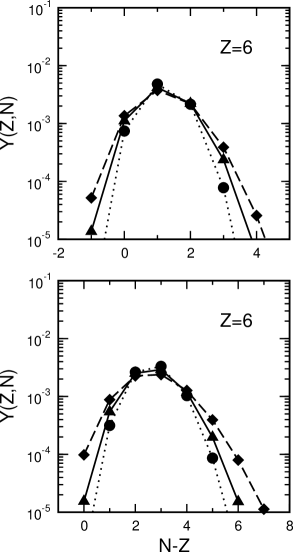
Figure 2: Calculated isotopic yields of $Z=6$–fragment with the “superstiff” symmetry term (diamonds) and the “soft” symmetry term (triangles). The circles represent the results obtained neglecting the contribution of isovector-like fluctuations in the “soft” case. The values of $\varrho$, ${\rm T}$, $L$, and $t$ are $\varrho=0.3\varrho_{eq}$, ${\rm T}=4.5\,{\rm MeV}$, $L=1.3\,r_{0}$, and $t=125\,{\rm fm}/c$. Top panel: $\alpha=0.1$, the value of the parameter $\gamma(t)$ is $\gamma(t)=1.02\,10^{-3}$ for the “superstiff” symmetry term, for the “soft” symmetry term $\gamma(t)=0.69\,10^{-3}$ and $\gamma(t)=0.37\,10^{-3}$, with and without the contributions from the isovector–like fluctuations, respectively. Bottom panel: $\alpha=0.2$, the value of the parameter $\gamma(t)$ is $\gamma(t)=1.62\,10^{-3}$ for the “superstiff” symmetry term, for the “soft” symmetry term $\gamma(t)=0.89\,10^{-3}$ and $\gamma(t)=0.56\,10^{-3}$, with and without the contributions from the isovector–like fluctuations, respectively.

In Fig. 2 we report the isotopic yields of $Z=6$–fragment, calculated according to Eqs. (19) and (26) for two different values of the asymmetry: $\alpha=0.1$ and $\alpha=0.2$. The used values of the parameters ${\rm T}=4.5\,{\rm MeV}$, $\varrho=0.3\varrho_{eq}$ and $t=125\,{\rm fm}/c$, where $t$ is the time that the system spends in the instability region, are compatible with the analogous values obtained within the SMF approach of Ref. Bar02 . For the dynamical correlation length we have chosen the value $L=1.3\,r_{0}$. This value corresponds to the effective exponent $\tau_{eff}=1.65$ of the power law $Y(Z)=Y_{0}Z^{-\tau_{eff}}$ for fragment distribution Mat03 . In the figure we display the results obtained with the “superstiff” asymmetry term and with the “soft” asymmetry term of the nucleon–nucleon interaction. Moreover we compare also the relative contribution of isoscalar-like and isovector-like fluctuations to the width.

In the ”superstiff” case isovector–like oscillations are suppressed for the considered values of $\varrho$, $T$ and $\alpha$, i.e. Eq. (4) has only one pole, so the width comes essentially from the dispersion of the chemical effect in the isoscalar-like fluctuations (diamonds). In the “soft” case, the full calculation is represented by triangles, while the result obtained taking into account only the contribution from the isoscalar-like modes is represented by circles. Comparing diamonds and circles, we observe that the “superstiff” asymmetry term gives rise to a wider isotopic distribution. This is due to the fact that the “soft” asymmetry term, at the considered density, is more effective to drive fragments closer to the average asymmetry value, with respect to an asymmetry term with a stronger density dependence. Indeed we find that, in spite of the competition with Coulomb and surface effects, the isospin distillation mechanism does not change much with the wave number $k$, in the “soft” case. The counterpart in our formalism is that in this case the behaviors of the components of the covariance matrix, as functions of $k$, are more similar each other reducing the width of the isotopic distribution. However, adding the contributions due to the isovector-like fluctuations, the total width obtained in the “soft” case (triangles) becomes closer to the “superstiff” results. It is also possible to observe that the contribution of the isovector-like fluctuations to the full width is more important at smaller asymmetry. This is because isovector-like fluctuations become weaker when increasing the asymmetry of the matter.

Figure 2 also shows that the width of the isotopic yields increases with asymmetry. This corresponds to the general property that for more neutron–rich systems the density–density response function of neutrons is enhanced with respect to that of protons. In addition, we can see that the more neutron–rich system ($\alpha=0.2$) produces the more neutron–rich isotopes, as expected.

It is worth to remark that both the overall behavior and the widths of the distributions of Fig. 2 favourably compare with the corresponding distributions for primary fragments calculated within the SMF approach Liu04 .

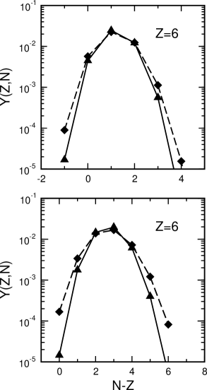
Figure 3: Isotopic distributions calculated according to the correlation volume prescription (Eq. 21). The values of the parameters and the symbols are the same as in Fig 2.

In Fig. 3 we present isotopic distributions obtained using the correlation volume prescription (Eq. 21), with ${\bar{A}}=20$. This value corresponds to the average size of intermediate mass fragments, as obtained in the considered conditions of density and temperature. As one can see by comparing Figs. 2 and 3, results are not very different with the two prescriptions.

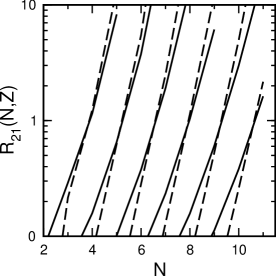
Figure 4: Isotopic ratio $R_{21}(N,Z)=Y_{\alpha=0.2}(N,Z)/Y_{\alpha=0.1}(N,Z)$ calculated with the “superstiff” symmetry term (solid lines ) and with the “soft” symmetry term (dashed lines). Lines correspond to different values of $Z$, $Z=3-8$ from left to right. The values of remaining parameters are the same as in Fig 2.

The ratio between isotopic yields observed in two different reactions, $R_{21}(N,Z)=Y_{\alpha_{2}}(N,Z)/Y_{\alpha_{1}}(N,Z)$, shows a very simple behavior. As a function of $Z$ and $N$, it can well be fitted by an exponential law (the so called isoscaling relationship) Xu00 ; Tsa01 ; Tan01 ; Tsa101 . In addition, the isoscaling relationship has been reproduced by SMF–model calculations also for the distributions of primary fragments Liu04 . This particular feature of the isotopic distributions can represent an effective tool to compare isotopic distributions from systems with different $N/Z$ ratios.

The isotopic ratio $R_{21}(N,Z)$ calculated in our approach, according to Eqs. (19) and (26), for two different values of the asymmetry parameter, $\alpha_{2}=0.2$ and $\alpha_{1}=0.1$, is displayed in Figs. 4 and 5. In Fig. 4 we compare the values of $R_{21}(N,Z)$ as a function of $N$, obtained with the “superstiff” symmetry term and with the “soft” symmetry term. The linear behavior, in logaritmic scale, with the same slope for every $Z$ is reproduced in both cases within a satisfying approximation. Because of the smaller value of the width parameter $\gamma(t)$, the “soft” symmetry term gives a steeper slope with respect to the “superstiff” term. The average values of the slope approximatively are $2.2\pm 0.2$ and $1.5\pm 0.15$ for the “soft” case and the “superstiff” case respectively.

Figure 5: Same as in Fig. 4 but using only the “superstiff” symmetry term and for two different values of the density: solid lines correspond to $\varrho=0.3\,\varrho_{eq}$ and $t=125\,{\rm fm}/c$, dashed lines correspond to $\varrho=0.4\,\varrho_{eq}$ and $t=150\,{\rm fm}/c$.

In Fig. 5 the ratio $R_{21}(N,Z)$ is displayed for two values of the density of the system at the break–up. In order to obtain fluctuations of similar magnitude in the two cases, two different times the system spends in the instability region are considered. Nevertheless, a behavior with a steeper slope is observed in the more unstable case. This is due to a smaller value of $\gamma(t)$ in this case, since, for a given charge asymmetry, the response functions of protons and of neutrons tend to be more similar with decreasing density.

We now perform a more quantitative comparison between predictions of our approach and results for primary fragments of the SMF–model calculations of Ref. Liu04 . To this purpose we adopt for the average asymmetry of fragments the values predicted by the SMF model for semicentral collisions of ${}^{112}{\rm Sn}+^{112}{\rm Sn}$ and ${}^{124}{\rm Sn}+^{124}{\rm Sn}$ Bar02 ; Liu04 : $\alpha_{1}=0.13$ and $\alpha_{2}=0.195$, respectively. In both the approaches the same “superstiff” symmetry term for the effective interaction is used. Also the values of density $\varrho=0.3\varrho_{eq}$, temperature ${\rm T}=4.5\,{\rm MeV}$, and time spent at the break–up $t=125\,{\rm fm}/c$ are chosen according to the results of SMF–model calculations. Figure 6 shows the isotopic ratio $R_{21}(N,Z)$ calculated with our approach and the curves obtained in Ref. Liu04 by fitting the results of the SMF model with an exponential law. We observe a remarkable agreement between the results of our nuclear matter calculations and the simulations of the SMF–model.

Figure 6: Comparison of calculated isotopic ratio $R_{21}(N,Z)=Y_{\alpha=0.195}(N,Z)/Y_{\alpha=0.13}(N,Z)$ (diamonds) with the fit for primary fragments of Ref. Liu04 (solid lines). From left to right $Z=3,4,5,6,7,8$. Calculations are done with the “superstiff” symmetry term. The values of density $\varrho$, temperature ${\rm T}$, time $t$, and ratio $L/r_{0}$ are the same as in Fig. 2.

IV Conclusions

In this article we discuss relevant observables of multifragmentation processes in charge asymmetric nuclear matter, such as the isotopic distribution of intermediate–mass fragments, as obtained within the spinodal decomposition scenario, on the basis of an analytical approach. Fragmentation happens due to the development of isoscalar-like unstable modes, i.e. unstable density oscillations with also a chemical component, leading to the formation of more symmetric fragments. We find that the isotopic distributions are peaked at a value given by the average distillation effect, while the width is determined by the dispersion of the chemical effect among the relevant unstable modes and by isovector-like fluctuations present in the matter that undergoes spinodal decomposition. The size of this dispersion is mostly due to the competition between symmetry energy effects (that favour the formation of symmetric fragments) and the Coulomb repulsion, that acts against the concentration of protons in large density domains, expecially for modes with large wavelength. Clearly the net result of this competion also depends on the EOS used. Smaller widths are obtained with a “soft” symmetry energy term. However, the contribution due to isovector-like fluctuations is more important in the “soft” case, indeed in the “superstiff” case isovector oscillations are suppressed. Hence finally the isotopic distributions are quite similar when using the two parameterizations of the symmetry energy.

In particular, we find that, when considering two systems with different asymmetry, the isotopic (or isotonic) yields obey an approximate isoscaling, with a slope connected to the difference betwen the asymmetries of the two systems and to the differences between the widths of the isotopic distributions. Hence isoscaling properties can be recovered in a dynamical picture. We notice that isoscaling has been found in dynamical simulations of heavy ion collisions, such as stochastic mean field Liu04 and antisymmetrized molecular dynamics calculations Ono .

The isoscaling parameters are also connected to the properties of the symmetry term in the EOS. Indeed we have seen that a stiffer behavior of the symmetry energy term yields larger isotopic widths, leading to smaller values of the slope (see Fig. 4). However, as reported in Ref. Bar02 , we also observe that in collisions of charge asymmetric systems, pre-equilibrium emission is less neutron rich when using a stiffer parametrization of the symmetry term (thus leading to more asymmetric fragments), with respect to the “soft” case. Therefore, in the isoscaling analysis, there could be a compensation between the average asymmetry of fragments (larger in the “stiff” case) and the width of the distribution (also larger in the “stiff” case). In fact, for the systems considered in Ref. Liu04 , similar values of the slope are obtained for the two parameterizations considered for the symmetry energy.

It may also be interesting to notice that the values obtained in our calculations are larger than the predictions of statistical multifragmentation models, see Ref. Tsa101 . Of course this picture can be modified by the secondary de-excitation process, that reduces the asymmetry of fragments and, consequently, the slopes deduced from isoscaling. Hence the final distributions can be quite different from the primary ones. A more detailed study, aiming to extract information on the primary distributions and on the fragmentation mechanism, would require the introduction of more sophisticated observables, probably based on an event by event analysis, in line with the recent investigations of correlations between intermediate–mass fragments Bor02 .

References

- (1) J. M. Lattimer and M. Prakash, Astrophys. J. 550, 426 (2001) and references therein.
- (2) H. Mueller and B. D. Serot, Phys. Rev. C 52, 2072 (1995).
- (3) Bao–An Li and C. M. Ko, Nucl. Phys. A618, 498 (1997).
- (4) V. Baran, M. Colonna, M. Di Toro, and A. B. Larionov, Nucl. Phys. A632, 287 (1998).
- (5) A. B. Larionov, A. S. Botvina, M. Colonna, and M. Di Toro, Nucl. Phys. A658, 375 (1999).
- (6) A. S. Botvina and I. N. Mishustin, Phys. Rev. C 63, 061601 (2001).
- (7) V. Baran, M. Colonna, M. Di Toro, and V. Greco, Phys. Rev. Lett. 86, 4492 (2001).
- (8) V. Baran, M. Colonna, M. Di Toro, V. Greco, M. Zielinska–Pfabè, and H. H. Wolter, Nucl. Phys. A703, 603 (2002).
- (9) H. S. Xu et al., Phys. Rev. Lett. 85, 716 (2000).
- (10) M. B. Tsang, W. A. Friedman, C. K. Gelbke, W. G. Lynch, G. Verde, and H. S. Xu, Phys. Rev. Lett. 86, 5023 (2001).
- (11) H. S. Xu et al., Phys. Rev. C 65, 061602 (2002).
- (12) E. Geraci et al., Nucl. Phys. A732, 173 (2004).
- (13) W. P. Tan, S. R. Souza, R. J. Charity, R. Donangelo, W. G. Lynch, and M. B. Tsang, Phys. Rev. C 68, 034609 (2003) and references therein.
- (14) F. Matera and A. Dellafiore, Phys. Rev. C 62, 044611 (2000).
- (15) F. Matera, A. Dellafiore, and G. Fabbri, Phys. Rev. C 67, 034608 (2003).
- (16) G. Fabbri and F. Matera, Phys. Rev. C 58, 1345 (1998).
- (17) S. Das Gupta, A. Z. Mekjian, and M. B. Tsang, in Advances in Nuclear Physics, edited by J. W. Negele and E. Vogt (Plenum, New York, 2001), Vol. 26, p. 91.
- (18) B. Borderie, J. Phys. G 28, R217 (2002).
- (19) Ph. Chomaz, M. Colonna, and J. Randrup, Phys. Rep. 389, 263 (2004).
- (20) M. Colonna, M. Di Toro, A. Guarnera, S. Maccarone, M. Zielinska–Pfabè, and H. H. Wolter, Nucl. Phys. A642, 449 (1998).
- (21) W. P. Tan, Bao–An Li, R. Donangelo, C. K. Gelbke, M.–J. van Goethem, X. D. Liu, W. G. Lynch, S. R. Souza, M. B. Tsang, G. Verde, A. Wagner, and H. S. Xu, Phys. Rev. C 64, 051901(R) (2001).
- (22) M. B. Tsang, C. K. Gelbke, X. D. Liu, W. G. Lynch, W. P. Tan, G. Verde, H. S. Xu, W. A. Friedman, R. Donangelo, S. R. Souza, C. B. Das, S. Das Gupta, and D. Zhabinsky, Phys. Rev. C 64, 054615 (2001).
- (23) T. X. Liu et al., Phys. Rev. C 69, 014603 (2004).
- (24) M. Colonna, Ph. Chomaz, and J. Randrup, Nucl. Phys. A567, 637 (1994).
- (25) C. W. Gardiner, Handbook of Stochastic Methods (Springer–Verlag, Berlin, 1997), Chap. 4.
- (26) J. D. Gunton, M. San Miguel, and Paramdeep S. Shani, in Phase Transitions and Critical Phenomena, edited by C. Domb and J.L. Lebowitz (Academic, London, 1983), Vol. 8, p. 267.
- (27) D. Kiderlen and H. Hofmann, Phys. Lett. B 353, 417 (1995); H. Hofmann and D. Kiderlen, Int. J. Mod. Phys. E 7, 243 (1998).
- (28) M. Colonna and Ph. Chomaz, Phys. Rev. C 49, 1908 (1994).
- (29) W. D. Myers and W. J. Swiatecki, Nucl. Phys. 81, 1 (1966).
- (30) G. Baym, H. A. Bethe, and C. J. Pethik, Nucl. Phys. A175, 225 (1971).
- (31) Bao–An Li, Phys. Rev. Lett. 85, 4221 (2000).
- (32) M. Colonna, M. Di Toro, G. Fabbri, and S. Maccarone, Phys. Rev. C 57, 1410 (1998).
- (33) M. Colonna, Ph. Chomaz and S. Ayik, Phys. Rev. Lett. 88, 122701 (2002).
- (34) B. Tamain and D. Durand, in Trends in Nuclear Physics, 100 years later, Proceedings of the Les Houches Summer School, Session 66, edited by H. Nifenecker, J.–P. Blaizot, G.F. Bertsch, W. Weise, and F. David (North–Holland, Amsterdam,1998), p. 295.
- (35) S. Ayik, Ph. Chomaz, M. Colonna, and J. Randrup, Z. Phys. A 355, 407 (1996).
- (36) Akira Ono, P. Danielewicz, W. A. Friedman, W. G. Lynch, and M. B. Tsang, Phys. Rev. C 68, 051601(R) (2003).