Benchmark calculation for proton-deuteron elastic scattering observables including Coulomb

Abstract

Two independent calculations of proton-deuteron elastic scattering observables including Coulomb repulsion between the two protons are compared in the proton lab energy region between 3 MeV and 65 MeV. The hadron dynamics is based on the purely nucleonic charge-dependent AV18 potential. Calculations are done both in coordinate space and momentum space. The coordinate-space calculations are based on a variational solution of the three-body Schrödinger equation using a correlated hyperspherical expansion for the wave function. The momentum-space calculations proceed via the solution of the Alt-Grassberger-Sandhas equation using the screened Coulomb potential and the renormalization approach. Both methods agree within 1% on all observables, showing the reliability of both numerical techniques in that energy domain. At energies below three-body breakup threshold the coordinate-space method remains favored whereas at energies higher than 65 MeV the momentum-space approach seems to be more efficient.

I Introduction

Although there is a long history of theoretical work on the solution of the Coulomb problem in three-particle scattering alt:78a ; berthold:90a ; kievsky:96a ; kievsky:01a ; chen:01a ; alt:02a ; suslov:04a , the work of Refs. kievsky:96a ; kievsky:01a pioneered the effort on fully converged numerical calculations for proton-deuteron $(pd)$ elastic scattering including the Coulomb repulsion between protons together with realistic nuclear interactions. In their work the authors use the charge-dependent AV18 potential together with the Urbana IX three-nucleon force and proceed to solve the three-particle Schrödinger equation using the Kohn variational principle (KVP); the wave function satisfies appropriate Coulomb distorted asymptotic boundary conditions and is expanded at short distances in a pair correlated hyperspherical harmonics basis set. The results presented were fully converged vis-à-vis the size of the basis set and the angular momentum states included in the calculation. In parallel a benchmark calculation was performed kievsky:01b where results obtained variationally were compared with those obtained from the solution of coordinate-space Faddeev equations for the AV14 potential at energies below three-body breakup threshold.

In a recent publication deltuva:05a the momentum-space solution of the Alt-Grassberger-Sandhas (AGS) equation alt:67a for two protons and a neutron was successfully applied, not only to $pd$ elastic scattering but also to radiative $pd$ capture and two-body electromagnetic disintegration of ${}^{3}\mathrm{He}$. The treatment of the Coulomb interaction is based on the ideas proposed by Taylor taylor:74a for two charged particle scattering and extended in LABEL:~alt:78a for three-particle scattering with two charged particles alone. The Coulomb potential is screened, standard scattering theory for short-range potentials is used, and the obtained results are corrected for the unscreened limit using the renormalization prescription taylor:74a ; alt:78a . The results presented in LABEL:~deltuva:05a are converged vis-à-vis the screening radius $R$ and the number of included two-body and three-body angular momentum states. Although in LABEL:~deltuva:05a the hadron dynamics is based on the purely nucleonic charge-dependent (CD) Bonn potential and its realistic coupled-channel extension CD Bonn + $\Delta$, allowing for single virtual $\Delta$-isobar excitation, other realistic potential models may be used easily as well.

Motivated by recent experimental efforts in the measurements of $pd$ elastic observables sagara:94a ; exp1 ; exp2 , in the present paper we present benchmark results for a number of $pd$ elastic scattering observables, both below and above three-body breakup threshold, using the charge-dependent AV18 wiringa:95a two-nucleon potential and no three-nucleon force. In Sec. II we make a short description of the methods we use, in Sec. III we present the results, and in Sec. IV the conclusions.

II The Methods

In this section we briefly introduce both methods and provide the basic framework for a general understanding of the technical procedures; further details may be found in the appropriate references. We choose to describe the method based on KVP using its traditional notation, which we attempt to carry over to the discussion of the integral equation approach in Sec. II.2 and III. Therefore the presentation of the integral equation approach will not be in the notation used in LABEL:~deltuva:05a .

II.1 The Kohn variational principle

The KVP can be used to describe nucleon-deuteron $(Nd)$ elastic scattering. Below the three-body breakup threshold the collision matrix is unitary and the problem can be formulated in terms of the real reactance matrix ($K$–matrix). Above the three-body breakup threshold the elastic part of the collision matrix is no longer unitary and the formulation in terms of the $S$-matrix, the complex form of the KVP, is convenient. Referring to Refs. kievsky:01a ; KRV99 ; VKR00 for details, a brief description of the method is given below. The scattering wave function (w.f.) $\Psi$ is written as sum of two terms

$$\Psi=\Psi_{C}+\Psi_{A}\$$ (1)

which carry the appropriate asymptotic boundary conditions. The first term, $\Psi_{C}$, describes the system when the three–nucleons are close to each other. For large interparticle separations and energies below the three-body breakup threshold it goes to zero, whereas for higher energies it must reproduce a three outgoing particle state. It is written as a sum of three Faddeev–like amplitudes corresponding to the three cyclic permutations of the particle indices. Each amplitude $\Psi_{C}({\bf x}_{i},{\bf y}_{i})$, where ${\bf x}_{i},{\bf y}_{i}$ are the Jacobi coordinates corresponding to the $i$-th permutation, has total angular momentum $JJ_{z}$ and total isospin $TT_{z}$ and is decomposed into channels using $LS$ coupling, namely

$$\Psi_{C}({\bf x}_{i},{\bf y}_{i}) = \sum_{\alpha=1}^{N_{c}}\phi_{\alpha}(x_{i},y_{i}){\cal Y}_{\alpha}(jk,i)$$ (2)

$${\cal Y}_{\alpha}(jk,i) = \Bigl{\{}\bigl{[}Y_{\ell_{\alpha}}(\hat{x}_{i})Y_{L_{\alpha}}(\hat{y}_{i})\bigr{]}_{\Lambda_{\alpha}}\bigl{[}s_{\alpha}^{jk}s_{\alpha}^{i}\bigr{]}_{S_{\alpha}}\Bigr{\}}_{JJ_{z}}\;\bigl{[}t_{\alpha}^{jk}t_{\alpha}^{i}\bigr{]}_{TT_{z}},$$ (3)

where $x_{i},y_{i}$ are the moduli of the Jacobi coordinates and ${\cal Y}_{\alpha}$ is the angular-spin-isospin function for each channel. The maximum number of channels considered in the expansion is $N_{c}$. The two-dimensional amplitude $\phi_{\alpha}$ is expanded in terms of the pair correlated hyperspherical harmonic basis KVR93 ; KVR94

$$\phi_{\alpha}(x_{i},y_{i})=\rho^{-5/2}f_{\alpha}(x_{i})\left[\sum_{K}u^{\alpha}_{K}(\rho){}^{(2)}P^{\ell_{\alpha},L_{\alpha}}_{K}(\phi_{i})\right]\ ,$$ (4)

where the hyperspherical variables, the hyperradius $\rho$ and the hyperangle $\phi_{i}$, are defined by the relations $x_{i}=\rho\cos{\phi}_{i}$ and $y_{i}=\rho\sin{\phi}_{i}$. The factor ${}^{(2)}P^{\ell,L}_{K}(\phi)$ is a hyperspherical polynomial and $f_{\alpha}(x_{i})$ is a pair correlation function introduced to accelerate the convergence of the expansion. For small values of the interparticle distance $f_{\alpha}(x_{i})$ is regulated by the $NN$ interaction whereas for large separations $f_{\alpha}(x_{i})\rightarrow 1$.

The second term, $\Psi_{A}$, in the variational wave function of Eq.(1) describes the asymptotic motion of a deuteron relative to the third nucleon. It can also be written as a sum of three amplitudes with the generic one having the form

$$\Omega^{\lambda}_{LSJ}({\bf x}_{i},{\bf y}_{i})=\sum_{l_{\alpha}=0,2}w_{l_{\alpha}}(x_{i}){\cal R}^{\lambda}_{L}(y_{i})\left\{\left[[Y_{l_{\alpha}}({\hat{x}}_{i})s_{\alpha}^{jk}]_{1}s^{i}\right]_{S}Y_{L}({\hat{y}}_{i})\right\}_{JJ_{z}}[t_{\alpha}^{jk}t^{i}]_{TT_{z}}\ ,$$ (5)

where $w_{l_{\alpha}}(x_{i})$ is the deuteron w.f. radial component in the state $l_{\alpha}=0,2$. In addition, $s_{\alpha}^{jk}=1,t_{\alpha}^{jk}=0$ and $L$ is the relative nucleon-deuteron angular momentum. The superscript $\lambda$ indicates the regular ($\lambda\equiv R$) or the irregular ($\lambda\equiv I$) solution. In the $pd$ $(nd)$ case, the functions ${\cal R}^{\lambda}$ are related to the regular or irregular Coulomb (spherical Bessel) functions. The functions $\Omega^{\lambda}$ can be combined to form a general asymptotic state ${}^{(2S+1)}L_{J}$

$$\Omega^{+}_{LSJ}({\bf x}_{i},{\bf y}_{i})=\Omega^{0}_{LSJ}({\bf x}_{i},{\bf y}_{i})+\sum_{L^{\prime}S^{\prime}}{}^{J}{\cal L}^{SS^{\prime}}_{LL^{\prime}}\Omega^{1}_{L^{\prime}S^{\prime}J}({\bf x}_{i},{\bf y}_{i})\ ,$$ (6)

where

$$\Omega^{0}_{LSJ}({\bf x}_{i},{\bf y}_{i})= u_{00}\Omega^{R}_{LSJ}({\bf x}_{i},{\bf y}_{i})+u_{01}\Omega^{I}_{LSJ}({\bf x}_{i},{\bf y}_{i})\ ,$$ (7)

$$\Omega^{1}_{LSJ}({\bf x}_{i},{\bf y}_{i})= u_{10}\Omega^{R}_{LSJ}({\bf x}_{i},{\bf y}_{i})+u_{11}\Omega^{I}_{LSJ}({\bf x}_{i},{\bf y}_{i})\ .$$ (8)

The matrix elements $u_{ij}$ can be selected according to the four different choices of the matrix ${\cal L}=$ $K$-matrix, $K^{-1}$-matrix, $S$-matrix or $T$-matrix. A general three-nucleon scattering w.f. for an incident state with relative angular momentum $L$, spin $S$ and total angular momentum $J$ is

$$\Psi^{+}_{LSJ}=\sum_{i=1,3}\left[\Psi_{C}({\bf x}_{i},{\bf y}_{i})+\Omega^{+}_{LSJ}({\bf x}_{i},{\bf y}_{i})\right]\ ,$$ (9)

and its complex conjugate is $\Psi^{-}_{LSJ}$. A variational estimate of the trial parameters in the w.f. $\Psi^{+}_{LSJ}$ can be obtained by requiring, in accordance with the generalized KVP, that the functional

$$[{}^{J}{\cal L}^{SS^{\prime}}_{LL^{\prime}}]={}^{J}{\cal L}^{SS^{\prime}}_{LL^{\prime}}-{\frac{2}{{\rm det}(u)}}\langle\Psi^{-}_{LSJ}|H-E|\Psi^{+}_{L^{\prime}S^{\prime}J}\rangle\ ,$$ (10)

be stationary. Below the three-body breakup threshold, due to the unitarity of the $S$-matrix, the four forms for the ${\cal L}$-matrix are equivalent. However, it was shown that when the complex form of the principle is used, there is a considerable reduction of numerical instabilities kiev97 . Above the three-body breakup threshold it is convenient to formulate the variational principle in terms of the $S$–matrix. Accordingly, we get the following functional:

$$[{}^{J}{S}^{SS^{\prime}}_{LL^{\prime}}]={}^{J}{S}^{SS^{\prime}}_{LL^{\prime}}+{i}\langle\Psi^{-}_{LSJ}|H-E|\Psi^{+}_{L^{\prime}S^{\prime}J}\rangle\ .$$ (11)

The variation of the functional with respect to the hyperradial functions $u^{\alpha}_{K}(\rho)$ leads to the following set of coupled equations:

$$\sum_{\alpha^{\prime},k^{\prime}}\Bigl{[}A^{\alpha\alpha^{\prime}}_{kk^{\prime}}({\rho}){d^{2}\over d{\rho}^{2}}+B^{\alpha\alpha^{\prime}}_{kk^{\prime}}({\rho}){d\over d{\rho}}+C^{\alpha\alpha^{\prime}}_{kk^{\prime}}({\rho})+{M_{N}\over\hbar^{2}}E\;N^{\alpha\alpha^{\prime}}_{kk^{\prime}}({\rho})\Bigr{]}u^{\alpha^{\prime}}_{k^{\prime}}({\rho})=D^{\lambda}_{\alpha k}(\rho)\ .$$ (12)

For each asymptotic state ${}^{(2S+1)}L_{J}$ two different inhomogeneous terms are constructed corresponding to the asymptotic $\Omega^{\lambda}_{LSJ}$ functions with $\lambda\equiv 0,1$. Accordingly, two sets of solutions are obtained and combined to minimize the functional (11) with respect to the $S$-matrix elements. This is the first order solution, the second order estimate of the $S$-matrix is obtained after replacing the first order solution in Eq.(11).

In order to solve the above system of equations appropriate boundary conditions must be specified for the hyperradial functions. For energies below the three-body breakup threshold they go to zero when $\rho\rightarrow\infty$, whereas for higher energy they asymptotically describe the breakup configuration. The boundary conditions to be applied in this case have been discussed in Refs. kievsky:01a ; VKR00 ; KVR97 and are briefly illustrated below. To simplify the notation let us label the basis elements with the index $\mu\equiv[{\alpha},K]$, and introduce the completely antisymmetric correlated spin-isospin-hyperspherical basis element ${\cal Q}_{\mu}(\rho,\Omega)$ as linear combinations of the products

$$\sum_{i=1}^{3}f_{\alpha}(x_{i})\;{}^{(2)}P^{\ell_{\alpha},L_{\alpha}}_{K}(\phi_{i}){\cal Y}_{\alpha}(jk,i)\ ,$$ (13)

which depend on $\rho$ through the correlation factor. In terms of the ${\cal Q}_{\mu}(\rho,\Omega)$ the internal part is written as

$$\Psi_{C}=\rho^{-5/2}\sum_{\mu=1}^{N_{m}}\omega_{\mu}(\rho){\cal Q}_{\mu}(\rho,\Omega)\ ,$$ (14)

with $N_{m}$ the total number of basis functions considered. The hyperradial functions $u_{\mu}(\rho)$ and $\omega_{\mu}(\rho)$ are related by an unitary transformation imposing that the “uncorrelated” basis elements ${\cal Q}^{0}_{\mu}(\Omega)$, obtained by setting all the correlation functions $f_{\alpha}(x_{i})=1$, form an orthogonal basis. Explicitly, the matrix elements of the norm $N$ behave as

$$N_{\mu\mu^{\prime}}(\rho)=\int d\Omega\;{\cal Q}_{\mu}(\rho,\Omega)^{\dagger}{\cal Q}_{\mu^{\prime}}(\rho,\Omega)\rightarrow N^{(0)}_{\mu\mu^{\prime}}+{N^{(3)}_{\mu\mu^{\prime}}\over\rho^{3}}+{\cal O}(1/\rho^{5})\ ,\qquad{\rm for\ }\rho\rightarrow\infty\ ,$$ (15)

where, in particular,

$$N^{(0)}_{\mu\mu^{\prime}}=\int d\Omega\;{\cal Q}^{0}_{\mu}(\Omega)^{\dagger}{\cal Q}^{0}_{\mu^{\prime}}(\Omega)\ .$$ (16)

is diagonal with diagonal elements ${\cal N}_{\mu}$ either $1$ or $0$. Therefore, some correlated elements have the property: ${\cal Q}_{\mu}(\rho,\Omega)\rightarrow 0$ as $\rho\rightarrow\infty$. In the following we arrange the new basis in such a way that for values of the index $\mu\leq\overline{N}_{m}$ the eigenvalues of the norm are ${\cal N}_{\mu}=1$ and for $\overline{N}_{m}+1\leq\mu\leq N_{m}$ they are ${\cal N}_{\mu}=0$.

For $\rho\rightarrow\infty$, neglecting terms going to zero faster than $\rho^{-2}$, the asymptotic expression of the set of Eqs.(12) rotated using the unitary transformation defined above, reduces to the form

$$\sum_{\mu^{\prime}}\biggl{\{}-{\hbar^{2}\over M_{N}}\left({d^{2}\over d\rho^{2}}-{{\cal K}_{\mu}({\cal K}_{\mu}+1)\over\rho^{2}}+Q^{2}\right){\cal N}_{\mu}\delta_{\mu,\mu^{\prime}}+{2\;Q\;\chi_{\mu\mu^{\prime}}\over\rho}\;+{\cal O}({1\over\rho^{3}})\biggr{\}}\omega_{\mu^{\prime}}(\rho)=0\ ,$$ (17)

where $E=\hbar^{2}Q^{2}/M_{N}$ and ${\cal K}_{\mu}=G_{\mu}+3/2$. Here $G_{\mu}$ is the grand-angular quantum number defined as $G_{\mu}=l_{\alpha}+L_{\alpha}+2K$ and the matrix $\chi$ is defined as

$${\chi}_{\mu\mu^{\prime}}=\int d\Omega\;{\cal Q}^{0}_{\mu}(\Omega)^{\dagger}\;\hat{\chi}\;{\cal Q}^{0}_{\mu^{\prime}}(\Omega)\ .$$ (18)

The dimensionless operator $\hat{\chi}$ originates from the Coulomb interaction as

$$\hat{\chi}={M_{N}\over 2\hbar^{2}Q}\sum_{i=1}^{3}{e^{2}\over\cos\phi_{i}}{1+\tau_{j,z}\over 2}{1+\tau_{k,z}\over 2}\ .$$ (19)

It should be noticed that $\chi_{\mu\mu^{\prime}}=0$ if $\mu,\mu^{\prime}>{\overline{N}_{m}}$.

In practice, the functions $\omega_{\mu}(\rho)$ are chosen to be regular at the origin, i.e. $\omega_{\mu}(0)=0$ and, in accordance with the equations to be satisfied for $\rho\rightarrow\infty$, to have the following behavior ($\mu\leq\overline{N}_{m}$)

$$\omega_{\mu}(\rho)\rightarrow-\sum_{\mu^{\prime}=1}^{\overline{N}_{m}}\left(e^{-i{\hat{\chi}}\ln 2Q\rho}\right)_{\mu\mu^{\prime}}\;b_{\mu^{\prime}}\;e^{iQ\rho}\ ,$$ (20)

where $b_{\mu^{\prime}}$ are unknown coefficients. This form corresponds to the asymptotic behavior of three outgoing particles interacting through the Coulomb potential merkuriev2 . In the case of $nd$ scattering ($\chi\equiv 0$) the outgoing solutions evolve as outgoing Hankel functions $H^{(1)}(Q\rho)$ ($\omega_{\mu}(\rho)\rightarrow-b_{\mu}e^{iQ\rho}$).

For values of the index $\mu>\overline{N}_{m}$ the eigenvalues of the norm are ${\cal N}_{\mu}=0$ and the leading terms in Eq.(17) vanish. So, the asymptotic behavior of these $\omega_{\mu}$ functions is governed by the next order terms. However, for $\mu>\overline{N}_{m}$, it is verified that $\omega_{\mu}{\cal Q}_{\mu}\rightarrow 0$ as $\rho\rightarrow\infty$.

In order to solve the system of Eqs.(12) the hyperradial functions are expanded in terms of Laguerre polynomials plus an auxiliary function

$$\omega_{\mu}(\rho)=\rho^{5/2}\sum_{m=0}^{M}A^{m}_{\mu}L^{(5)}_{m}(z)\exp(-{z\over 2})+A^{M+1}_{\mu}\overline{\omega}_{\mu}(\rho)\ ,$$ (21)

where $z=\gamma\rho$ and $\gamma$ is a nonlinear parameter. The linear parameters $A^{m}_{\mu}$ $(m=0,....,M+1)$ are determined by the variational procedure.

The inclusion of the auxiliary functions $\overline{\omega}_{\mu}(\rho)$ defined in Eq.(21) is useful for reproducing the oscillatory behavior shown by the hyperradial functions for $\rho\gtrsim 30$ fm. Otherwise a rather large number $M$ of polynomials should be included in the expansion. A convenient choice is to take them as the regular solutions of a one dimensional differential equation corresponding to the $\mu$-th equation of the system whose asymptotic behavior is the one of Eq.(17). In the cases considered here the solutions obtained for the $S$-matrix stabilize for values of the matching radius $\rho_{0}>100$ fm.

II.2 The integral equation approach

The integral equation to be solved is the AGS equation alt:67a for three-particle scattering where each pair of nucleons interacts through the strong potential $v$ and the Coulomb potential $w$ acts only between charged nucleons. The work in LABEL:~deltuva:05a follows the seminal work of Refs. taylor:74a ; alt:78a in the sense that the treatment of the Coulomb interaction is based on screening, followed by the use of standard scattering theory for short-range potentials and renormalization of the obtained results in order to correct for the unscreened limit. Nevertheless there are important differences relative to LABEL:~alt:02a that are paramount to the fast convergence of the calculation in terms of screening radius R and the effective use of realistic interactions:

a) We work with a screened Coulomb potential

$$w_{R}(r)=w(r)\;e^{-(r/R)^{n}}$$ (22)

where $w(r)=\frac{\alpha}{r}$ is the true Coulomb potential, $\alpha$ being the fine structure constant and $n$ a power controlling the smoothness of the screening. We prefer to work with a sharper screening than the Yukawa screening $(n=1)$ of LABEL:~alt:02a because we want to ensure that the screened Coulomb potential $w_{R}$ approximates well the true Coulomb one $w$ for distances $r<R$ and simultaneously vanishes rapidly for $r>R$, providing a comparatively rapid convergence of the partial wave expansion. In contrast, the sharp cutoff $(n\to\infty)$ yields unpleasant oscillatory behavior in momentum space representation, leading to convergence problems. We find values $3\leq n\leq 6$ to provide a sufficient smoothness and fast convergence; $n=4$ is used for the calculations of this paper.

b) Although the choice of the screened potential improves the partial wave convergence, the practical implementation of the solution of AGS equation still places a technical difficulty, i.e., the calculation of the AGS operators for nuclear plus screened Coulomb potentials requires two-nucleon partial waves with pair orbital angular momentum considerably higher than required for the hadronic potential alone. In this context the perturbation theory for higher two-nucleon partial waves developed in Ref. deltuva:03b is a very efficient and reliable technical tool for treating the screened Coulomb interaction in high partial waves.

As a result of these two technical implementations, the method deltuva:03a that was developed before for solving three-particle AGS equations without Coulomb could be successfully used in the presence of screened Coulomb. Using the usual three-body notation, the full multichannel transition matrix reads

$$\begin{aligned} U^{(R)}_{\beta\alpha}(Z)={}&\bar{\delta}_{\beta\alpha}G_{0}^{-1}(Z)+\sum_{\sigma}\bar{\delta}_{\beta\sigma}T^{(R)}_{\sigma}(Z)G_{0}(Z)U^{(R)}_{\sigma\alpha}(Z),\end{aligned}$$ (23a)

where the superscript $$(R) R G_{0}(Z)=(Z-H_{0})^{-1} \bar{\delta}_{\beta\alpha}=1-\delta_{\beta\alpha}$$ denotes the dependence on the screening radius of the Coulomb potential, the free resolvent, , and

$$\begin{aligned} T^{(R)}_{\alpha}(Z)={}&(v_{\alpha}+w_{\alpha R})+(v_{\alpha}+w_{\alpha R})G_{0}(Z)T^{(R)}_{\alpha}(Z).\end{aligned}$$ (23b)

The two-particle transition matrix $T^{(R)}_{\alpha}(Z)$ results from the nuclear interaction $v_{\alpha}$ between hadrons plus the screened Coulomb $w_{\alpha R}$ between charged nucleons ($w_{\alpha R}=0$ otherwise). As expected the full multichannel transition matrix $U^{(R)}_{\beta\alpha}(Z)$ must contain the pure Coulomb transition matrix $T^{\mathrm{c\!\>\!.m\!\>\!.}}_{\alpha R}(Z)$ derived from the screened Coulomb $W^{\mathrm{c\!\>\!.m\!\>\!.}}_{\alpha R}$ between the spectator proton and the center of mass (c.m.) of the remaining neutron-proton $(np)$ pair in channel $\alpha$

$$T^{\mathrm{c\!\>\!.m\!\>\!.}}_{\alpha R}(Z)=W^{\mathrm{c\!\>\!.m\!\>\!.}}_{\alpha R}+W^{\mathrm{c\!\>\!.m\!\>\!.}}_{\alpha R}G^{(R)}_{\alpha}(Z)T^{\mathrm{c\!\>\!.m\!\>\!.}}_{\alpha R}(Z),$$ (24)

where $W^{\mathrm{c\!\>\!.m\!\>\!.}}_{\alpha R}=0$ for $n(pp)\;\;\alpha$ channels and $G^{(R)}_{\alpha}$ the channel resolvent

$$G^{(R)}_{\alpha}(Z)=(Z-H_{0}-v_{\alpha}-w_{\alpha R})^{-1}.$$ (25)

In a system of two charged particles and a neutral one, when $w_{\alpha R}=0$, $\;W^{\mathrm{c\!\>\!.m\!\>\!.}}_{\alpha R}\neq 0$ and vice versa.

As demonstrated in Refs. alt:78a ; deltuva:05a the split of the multichannel transition matrix

$$U^{(R)}_{\beta\alpha}(Z)=\delta_{\beta\alpha}T^{\mathrm{c\!\>\!.m\!\>\!.}}_{\alpha R}(Z)+[U^{(R)}_{\beta\alpha}(Z)-\delta_{\beta\alpha}T^{\mathrm{c\!\>\!.m\!\>\!.}}_{\alpha R}(Z)]$$ (26)

into a long-range part $\delta_{\beta\alpha}T^{\mathrm{c\!\>\!.m\!\>\!.}}_{\alpha R}(Z)$ and a Coulomb distorted short-range part $[U^{(R)}_{\beta\alpha}(Z)-\delta_{\beta\alpha}T^{\mathrm{c\!\>\!.m\!\>\!.}}_{\alpha R}(Z)]$ is extremely convenient to recover the unscreened Coulomb limit. According to Refs. alt:78a ; deltuva:05a the full $pd$ transition amplitude $\langle\phi_{\beta}({\mathbf{q}}_{f})\nu_{\beta_{f}}|U_{\beta\alpha}|\phi_{\alpha}({\mathbf{q}}_{i})\nu_{\alpha_{i}}\rangle$ for the initial and final channel states with relative $pd$ momentum ${\mathbf{q}}_{i}$ and ${\mathbf{q}}_{f}$, $q_{f}=q_{i}$, energy $E_{\alpha}(q_{i})$, and discrete quantum numbers $\nu_{\alpha_{i}}$ and $\nu_{\beta_{f}}$, is obtained via the renormalization of the on-shell $U^{(R)}_{\beta\alpha}(Z)$ with $Z=E_{\alpha}(q_{i})+i0$ in the infinite $R$ limit. For the screened Coulomb transition matrix $T^{\mathrm{c\!\>\!.m\!\>\!.}}_{\alpha R}(Z)$, contained in $U^{(R)}_{\beta\alpha}(Z)$, that limit can be carried out analytically, yielding the proper Coulomb transition amplitude $\langle\phi_{\beta}({\mathbf{q}}_{f})\nu_{\beta_{f}}|T^{\mathrm{c\!\>\!.m\!\>\!.}}_{\alpha C}|\phi_{\alpha}({\mathbf{q}}_{i})\nu_{\alpha_{i}}\rangle$ alt:78a ; taylor:74a , while the Coulomb distorted short-range part requires the explicit use of a renormalization factor,

$$\begin{split}\langle\phi_{\beta}({\mathbf{q}}_{f})&\nu_{\beta_{f}}|U_{\beta\alpha}|\phi_{\alpha}({\mathbf{q}}_{i})\nu_{\alpha_{i}}\rangle\\ ={}&\delta_{\beta\alpha}\langle\phi_{\beta}({\mathbf{q}}_{f})\nu_{\beta_{f}}|T^{\mathrm{c\!\>\!.m\!\>\!.}}_{\alpha C}|\phi_{\alpha}({\mathbf{q}}_{i})\nu_{\alpha_{i}}\rangle\\ &+\lim_{R\to\infty}\{\mathcal{Z}_{R}^{-\frac{1}{2}}(q_{f})\langle\phi_{\beta}({\mathbf{q}}_{f})\nu_{\beta_{f}}|[U^{(R)}_{\beta\alpha}(E_{\alpha}(q_{i})+i0)\\ &-\delta_{\beta\alpha}T^{\mathrm{c\!\>\!.m\!\>\!.}}_{\alpha R}(E_{\alpha}(q_{i})+i0)]|\phi_{\alpha}({\mathbf{q}}_{i})\nu_{\alpha_{i}}\rangle\mathcal{Z}_{R}^{-\frac{1}{2}}(q_{i})\}.\end{split}$$ (27)

The renormalization factor

$$\mathcal{Z}_{R}(q)=e^{-2i\phi_{R}(q)},$$ (28a)

contains a phase $$\phi_{R}(q) pd L R$$ which, though independent of the relative orbital momentum in the infinite limit, is given by taylor:74a

$$\phi_{R}(q)=\sigma_{L}(q)-\eta_{LR}(q),$$ (28b)

where $\eta_{LR}(q)$ is the diverging screened Coulomb phase shift corresponding to standard boundary conditions, and $\sigma_{L}(q)$ the proper Coulomb phase referring to logarithmically distorted Coulomb boundary conditions. The limit of the Coulomb distorted short-range part of the multichannel transition matrix $[U^{(R)}_{\beta\alpha}(Z)-\delta_{\beta\alpha}T^{\mathrm{c\!\>\!.m\!\>\!.}}_{\alpha R}(Z)]$ has to be performed numerically but, due to its short-range nature, the limit is reached with sufficient accuracy at finite screening radii $R$. Furthermore, due to the choice of screening and perturbation technique to deal with high angular momentum states, $[U^{(R)}_{\beta\alpha}(Z)-\delta_{\beta\alpha}T^{\mathrm{c\!\>\!.m\!\>\!.}}_{\alpha R}(Z)]$ is calculated through the numerical solution of Eqs. (23) and (24), using partial-wave expansion.

In actual calculations we use the isospin formulation and, therefore, the nucleons are considered identical. Instead of Eq. (23a) we solve a symmetrized AGS equation

$$U^{(R)}(Z)=PG_{0}^{-1}(Z)+PT^{(R)}_{\alpha}(Z)G_{0}(Z)U^{(R)}(Z),$$ (29)

$P$ being the sum of the two cyclic three-particle permutation operators, and use a properly symmetrized $pd$ transition amplitude

$$\begin{split}\langle\phi_{\alpha}({\mathbf{q}}_{f})&\nu_{\alpha_{f}}|U|\phi_{\alpha}({\mathbf{q}}_{i})\nu_{\alpha_{i}}\rangle\\ ={}&\langle\phi_{\alpha}({\mathbf{q}}_{f})\nu_{\alpha_{f}}|T^{\mathrm{c\!\>\!.m\!\>\!.}}_{\alpha C}|\phi_{\alpha}({\mathbf{q}}_{i})\nu_{\alpha_{i}}\rangle\\ &+\lim_{R\to\infty}\{\mathcal{Z}_{R}^{-\frac{1}{2}}(q_{f})\langle\phi_{\alpha}({\mathbf{q}}_{f})\nu_{\alpha_{f}}|[U^{(R)}(E_{\alpha}(q_{i})+i0)\\ &-T^{\mathrm{c\!\>\!.m\!\>\!.}}_{\alpha R}(E_{\alpha}(q_{i})+i0)]|\phi_{\alpha}({\mathbf{q}}_{i})\nu_{\alpha_{i}}\rangle\mathcal{Z}_{R}^{-\frac{1}{2}}(q_{i})\}\end{split}$$ (30)

for the calculation of observables. For further technical details we refer to LABEL:~deltuva:05a .

III Results

In this section we compare numerical calculations for a number of elastic observables performed using the KVP and the integral equation approach. Three different lab energies have been considered: $3$, $10$, and $65$ MeV. The Coulomb effects are expected to be sizable in most of the observables at the first two energies. The two methods use a different scheme to construct the scattering states with total angular momentum and parity $J^{\pi}$. In the KVP the $LS$ coupling is used and channels are ordered by increasing values of $\ell_{\alpha}+L_{\alpha}$. The expansion of the scattering state is truncated at values $\ell_{\alpha}+L_{\alpha}=L_{max}+2$, where $L_{max}$ is the maximum value of $L$ corresponding to the asymptotic states ${}^{(2S+1)}L_{J}$. In the integral equation approach the $jj$ scheme has been used. The channels have been ordered for increasing values of the two-body angular momentum $j$ and for the strong interaction the maximum value $j_{max}=5$ has been considered for the first two energies whereas at $65$ MeV the value $j_{max}=6$ has been used; the screened Coulomb interaction is taken into account up to $j_{max}=25$ as described in LABEL:~deltuva:05a . Both numerical calculations presented here are converged relative to the number of three-body partial waves. In addition, the variational calculations are converged relative to the size of the hyperspherical basis set and, in the integral equation approach, the results are converged with respect to the screening radius $R$.

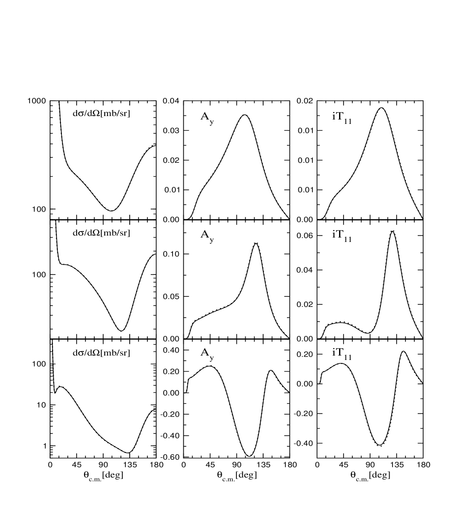
Figure 1: Differential cross section, and the proton and deuteron analyzing powers $A_{y}$ and $iT_{11}$ are shown for $pd$ elastic scattering at $3$ MeV (first row), $10$ MeV (second row) and $65$ MeV (third row) lab energies as functions of the c.m. scattering angle. Results obtained using KVP (thin solid line) and integral equation approach (dotted line) are compared.

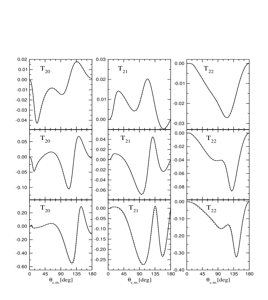
Figure 2: Tensor analyzing powers $T_{20}$, $T_{21}$, and $T_{22}$ are shown for $pd$ elastic scattering at $3$ MeV (first row), $10$ MeV (second row) and $65$ MeV (third row) lab energies as functions of the c.m. scattering angle. Results obtained using KVP (thin solid line) and integral equation approach (dotted line) are compared.

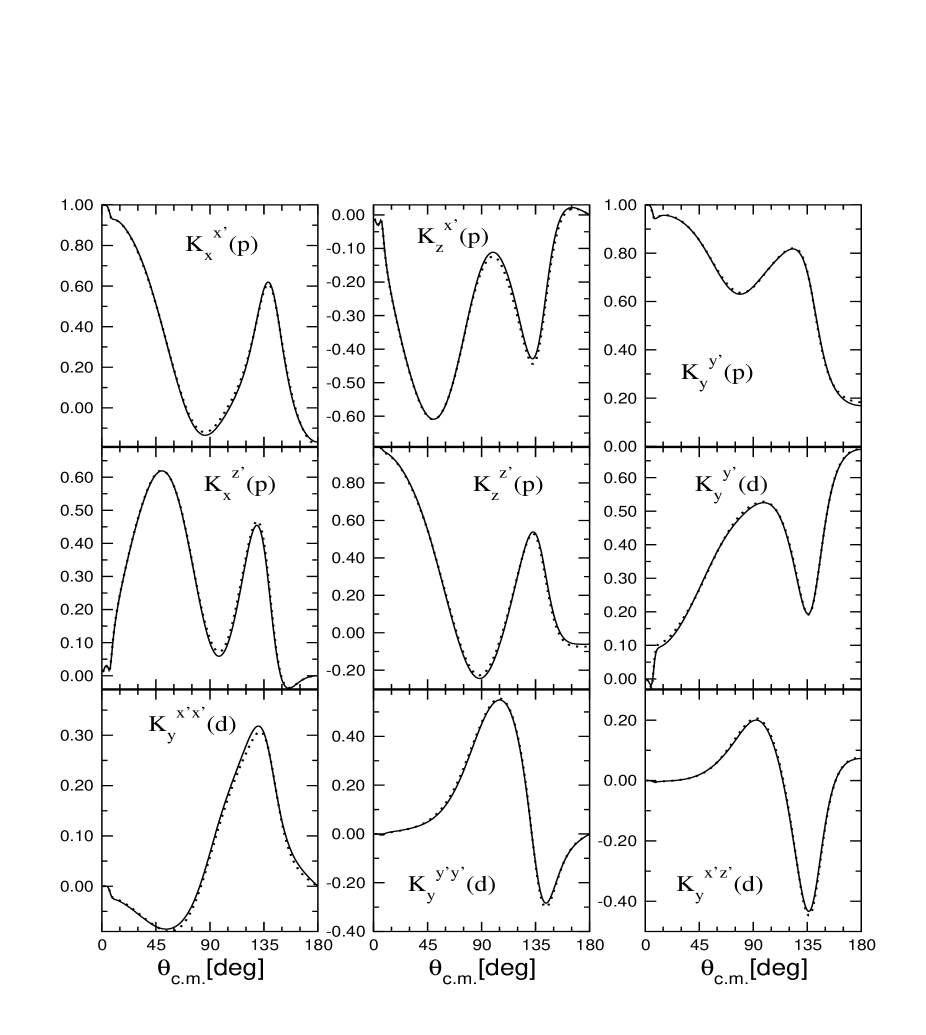
Figure 3: A selection of proton to proton and proton to deuteron spin transfer coefficients for $pd$ elastic scattering at $65$ MeV lab energy as function of the c.m. scattering angle. Results obtained using KVP (thin solid line) and integral equation approach (dotted line) are compared.

In Figs. 1 and 2 we compare the differential cross section and vector and tensor analyzing powers for $pd$ elastic scattering at the three selected energies, $3$, $10$ and $65$ MeV proton lab energies. In Fig. 3 a selection of spin transfer coefficients at $65$ MeV is shown. In the figures, two different curves are shown corresponding to calculations using the KVP (thin solid line) and integral equation approach (dotted line). By inspection of the figures one may conclude that the agreement is excellent because the numerical calculations agree to better than 1%. In fact the curves are practically one on top of the other, the exceptions being the maximum of $T_{21}$ and some spin transfer coefficients at $65$ MeV in which a small disagreement is observed. Nevertheless, it is important to mention that in all cases the difference between the two curves is smaller than the experimental accuracy for the corresponding data sets. Likewise the agreement between the two calculations largely exceeds the agreement of any of them with the data as shown in Refs. kievsky:01a ; deltuva:05a .

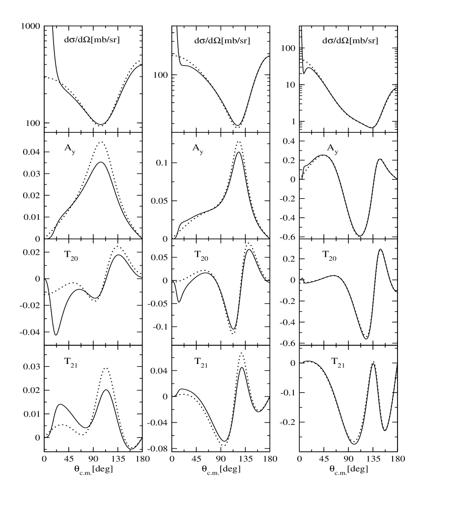
Figure 4: Calculations for $pd$ (solid line) and $nd$ (dotted line) scattering are compared for differential cross section, $A_{y}$, $T_{20}$ and $T_{21}$ at $3$ MeV (first column), $10$ MeV (middle column) and $65$ MeV (last column) nucleon lab energies.

The present results can be used to study Coulomb effects by comparing $nd$ to $pd$ calculations. In Fig. 4 we analyze the evolution of the Coulomb effects for the differential cross section, the nucleon analyzing power $A_{y}$ and two tensor analyzing powers, $T_{20}$ and $T_{21}$ at $3$, $10$ and $65$ MeV proton lab energies. In order to reduce the number of curves in the figure for the sake of clarity we present results obtained using the integral equation approach. The results obtained using the KVP for $nd$ scattering agree at the same level already shown for the $pd$ case in the previous figures. In Fig. 4 the thin solid line denotes the $pd$ calculation whereas the dotted line denotes the corresponding $nd$ calculation. The latter agrees well with the results of other existing $nd$ calculations witala:pc . From the figure we observe that Coulomb effects are appreciable at $3$ and $10$ MeV but are considerably reduced at $65$ MeV. A more exhaustive analysis on Coulomb effects can be found in Refs. kievsky:01a ; KRV01 ; deltuva:05a .

In addition to the benchmark comparison using AV18 potential we also give one result for the Malfliet-Tjon (MT) I-III potential, in order to resolve an existing problem. Reference suslov:04a reports a disagreement between $pd$ phase shifts results for MT I-III potential calculated using the first technique of this paper, the KVP kievsky:01a , and the configuration-space Faddeev equations suslov:04a . The calculation based on the second technique of this paper, the momentum-space integral equations deltuva:05a , clearly confirms the results of LABEL:~kievsky:01a . A detailed comparison of $pd$ and $nd$ phase shift results for MT I-III potential is given in Table 1.

In the following we discuss some of the limitations inherent to the two methods used to describe $pd$ elastic scattering. The KVP, as presented here, reduces the scattering problem to the solution of a linear set of equations in which the matrix elements of the Hamiltonian have to be computed between basis states; increasing the energy, appreciable contributions from states with high values of $\ell_{\alpha}+L_{\alpha}$ appear. In order to take into account these contributions, a very large basis has to be used with the consequence that numerical instabilities start to appear. In the integral equation approach at very low energies convergence in terms of screening radius requires $R>30\>\mathrm{fm}$, which in turn increases the number of two-body partial waves that are needed for convergence. The interplay of these two requirements makes the integral equation solution unstable at those very low energies. An interesting heuristic argument to understand the size of the screening radius needed for convergence is the wave length $\lambda$ corresponding to the on-shell momentum. At 3 MeV, 10 MeV, and 65 MeV proton lab energy, for which a screening radius of 20 fm, 10 fm, and 7 fm is needed for convergence, $\lambda$ is $24.8\>\mathrm{fm}$, $13.6\>\mathrm{fm}$, and $5.3\>\mathrm{fm}$, respectively. It appears that for the calculation of $pd$ elastic scattering observables the screening has to be only so large that one wave length can be accommodated in the Coulomb tail outside the range of the hadronic interaction; seeing proper Coulomb over one wave length appears enough to provide, with the additional help of renormalization, the true Coulomb characteristics of scattering despite screening.

IV Conclusions

In the present paper two methods devised to describe elastic $pd$ scattering are compared for a wide range of energies. One of the methods, the KVP, was developed a few years ago and used to study how realistic potential models, including two-body and three-body forces, describe the elastic observables measured for that reaction. On the other hand, numerical accurate results have been recently obtained solving the AGS equation for $pd$ scattering using a screened Coulomb potential corrected for the unscreened limit using a renormalization prescription. As has been briefly described in the present paper, both methods are substantially different. It is satisfactory to observe that both methods produce essentially the same results for a large variety of elastic observables using a realistic two-nucleon potential. We stress the fact that the selection of observables here presented is only part of the observables compared. In all cases, similar patterns have been obtained. In addition, by comparing the $pd$ calculations to the corresponding $nd$ calculations, Coulomb effects have been estimated. As expected these effects are sizable at low energies but at the highest analyzed energy, $65$ MeV, they are small, except at forward scattering angles. From these considerations it is possible to identify on a firm basis which $pd$ observables may or may not be analyzed by calculations in which the Coulomb interaction has been neglected.

We can conclude that at present it is possible to describe $pd$ elastic scattering, including the Coulomb repulsion, using standard techniques as the Faddeev equations in configuration and momentum space or variational principles. Moreover, in Ref. KVM04 the treatment of other terms of the $NN$ electromagnetic potential as the magnetic moment interaction has been discussed.

	${}^{2}\delta_{0}$	${}^{2}\eta_{0}$	${}^{4}\delta_{0}$	${}^{4}\eta_{0}$
$nd$ at 14.1 MeV	105.48	0.4649	68.95	0.9782
	105.49	0.4649	68.95	0.9782
$nd$ at 42.0 MeV	41.34	0.5022	37.72	0.9033
	41.36	0.5022	37.71	0.9033
$pd$ at 14.1 MeV	108.44	0.4984	72.60	0.9795
	108.39	0.4983	72.62	0.9796
$pd$ at 42.0 MeV	43.67	0.5056	39.95	0.9046
	43.70	0.5056	39.97	0.9046

Table 1: $nd$ and $pd$ phase-shift and inelasticity parameters calculated with MT I-III potential. For each reaction, the KVP and integral equation approach results are given in the first and second row, respectively.