$K\Lambda$ and $K\Sigma$ photoproduction in a coupled channels framework.

Abstract

A coupled channels analysis, based on the $\mathsf{K}$-matrix approach, is presented for photo-induced kaon production. It is shown that channel coupling effects are large and should not be ignored. The importance of contact terms in the analysis, associated with short range correlations, is pointed out. The extracted parameters are compared with $SU(3)$-model predictions.

I Introduction

One of the major issues of hadron physics is the determination of masses and coupling constants for the different baryon resonances. These extracted parameters serve as a test of different QCD-based models Met01 ; The01 . As will be demonstrated in this work, coupled channels effects are large and should be taken into account in extracting resonance parameters for the higher-lying resonances. Another reason for performing a coupled channels description is that the requirement of a simultaneous fit of the data for a multitude of observables in different reaction channels strongly confines the values of the model parameters thus reducing the model dependence to a minimum. The coupled-channel calculations presented here are based on an effective-field model which is gauge invariant and obeys the low-energy theorems.

However, as it was shown for example in ref. Pen02 , even the present large experimental database in a unitary coupled-channel effective Lagrangian model does not allow to uniquely fix the extracted parameters. One of the reasons for this is the necessity to include empirical form-factors in the model to regularize the matrix elements at higher energies. These form-factors introduce the need for a gauge-invariance restoration procedure. As is well known this has many ambiguities associated with it, see for example ref. Dav01 . In this work we will explicitly formulate these ambiguities in terms of four-point contact terms which can be added to the model Lagrangian. In particular we will show that procedure of minimal substitution, known as the Ohta prescription Ohta89 results in a major cancellation of the form-factor effects. This results in a large disagreement with the data, even in a coupled-channels description, which has the tendency to suppress the cross section at higher energies in a particular channel.

A number of analyses of data on strangeness production have been performed Tit02 ; Ire04 ; Jan02 ; Pen02 ; Benn01 , but only few of them are based on a coupled-channel model Pen02 . In addition different gauge-invariance restoration prescriptions are used, which makes it difficult to compare the parameters. In the present work we have investigated the implications of the different gauge-invariance restoration procedures, and formulated them in terms of additional gauge-invariant contact terms. In general these contact terms can be regarded as short-range effects which are not included in the model Lagrangian or due to loop corrections which have been omitted. In expressing the model dependence in terms of contact terms added to the model Lagrangian we follow the philosophy used in effective-field chiral perturbation theory Mei95 .

In the last years the data base on strangeness photoproduction SAPHIR1 ; SAPHIR2 has been extended appreciably. For certain kinematics these new data differs significantly from the old one. A new analysis is therefore appropriate.

II Model

This work is based on an effective Lagrangian model. The Lagrangian as used in the present calculation is given in the Appendix A and some of the main ingredients are presented in a following section. This Lagrangian is used to build the kernel for a $\mathsf{K}$-matrix approach. As described in the following section this allows to account for coupled channels effects while preserving many symmetries of a full field-theoretical approach.

II.1 $\mathsf{K}$-matrix model

In our calculation the coupled channels (or re-scattering) effects are included through the use of the $\mathsf{K}$-matrix formalism. In this section we present a short overview of the $\mathsf{K}$-matrix approach, a more detailed description can be found in ref. Kor98 ; Sch02 ; New82 .

In the $\mathsf{K}$-matrix formalism the scattering matrix is written as

$$\mathsf{T}=\frac{\mathsf{K}}{1-i\mathsf{K}}\,.$$ (1)

It is easy to check, that the resulting scattering amplitude $S=1+2i\mathsf{T}$ is unitary provided that $\mathsf{K}$ is Hermitian. The construction in Eq. (1) can be regarded as the re-summation of an infinite series of loop diagrams by making a series expansion,

$$\mathsf{T}=\mathsf{K}+i\mathsf{K}\mathsf{K}+i^{2}\mathsf{K}\mathsf{K}\mathsf{K}+\cdots\,.$$ (2)

The product of two $\mathsf{K}$-matrices can be rewritten as a sum of different one-loop contributions (three- and four-point vertex and self-energy corrections) depending on the Feynman diagrams which are included in the kernel, $\mathsf{K}$. However, not the full spectrum of loop corrections present in a true field-theoretical approach, is generated in this way and the missing ones should be accounted for in the kernel. In constructing the kernel one should be careful to prevent double counting. For this reason we include in the kernel tree-level diagrams only, modified with form-factors and contact terms. The contact terms (or four-point vertices) ensure gauge invariance of the model and express model-dependence in working with form factors, see Section III. Form factors and contact terms can be regarded as accounting for loop corrections which are not generated in the $\mathsf{K}$-matrix procedure, or for short-range effects which have been omitted from the interaction Lagrangian. Both s- and u-channel diagrams are included and the kernel thus obeys crossing symmetry.

Table 1: Baryon states included in the calculation of the kernel with their coupling constants. The column labelled W lists the decay width to states outside the model space. The columns labelled M and W are in units of GeV. See text for a discussion on the signs of the coupling constants.

$L_{IJ}$	M	W	$g_{N\pi}$	$g^{1}_{N\gamma}$	$g^{2}_{N\gamma}$	$g_{K\Lambda}$	$g_{K\Sigma}$	$g_{N\eta}$
$N$	$0.939$	$0.0$	$13.47$	—	—	$12$	$8.7$	$3.0$
$\Lambda$	$1.116$	$0.0$	—	—	—	—	—	—
$\Sigma$	$1.189$	$0.0$	—	—	—	—	—	—
$S_{11}$	$1.525$	$0.0$	$0.6$	$-1.2$	—	$0.1$	$0.0$	$2.0$
$S_{11}$	$1.690$	$0.030$	$1.0$	$-1.0$	—	$-0.1$	$0.0$	$-0.5$
$S_{31}$	$1.630$	$0.100$	$3.7$	$-0.25$	—	—	$-0.8$	—
$P_{11}$	$1.480$	$0.200$	$5.5$	$1.0$	—	$0.0$	$-2.0$	$0.0$
$P_{11}$	$1.750$	$0.300$	$3.0$	$0.3$	—	$0.0$	$-6.0$	$0.0$
$P_{13}$	$1.750$	$0.300$	$0.12$	$-0.5$	$2.0$	$-0.035$	$0.0$	$0.0$
$P_{33}$	$1.230$	$0.0$	$1.7$	$-2.2$	$-2.7$	—	$0.0$	—
$P_{33}$	$1.855$	$0.150$	$0.0$	$-0.4$	$-0.6$	—	$0.55$	—
$D_{13}$	$1.515$	$0.050$	$1.2$	$5.0$	$5.5$	$2.0$	$0.0$	$2.0$
$D_{13}$	$1.700$	$0.090$	$0.0$	$-1.0$	$0.0$	$0.0$	$0.3$	$0.0$
$D_{33}$	$1.670$	$0.250$	$0.8$	$1.5$	$0.6$	—	$-3.0$	—

Table 2: Mass, spin, parity and isospin of the mesons which are included in the model. The rightmost column specifies in which reaction channels their t-channel contribution are taken into account.

Meson	M [GeV]	$S^{\pi}$	$I$	t-ch contributions
$\pi$	$0.135$	$0^{-}$	$1$	($\gamma N\to\phi N$), ($\pi N\to\rho N$)
$K$	$0.494$	$0^{-}$	$\frac{1}{2}$	($\gamma N\to K\Lambda$), ($\gamma N\to K\Sigma$)
$\phi$	$1.019$	$1^{-}$	$0$
$\eta$	$0.547$	$0^{-}$	$0$	($\gamma N\to\phi N$)
$\rho$	$0.770$	$1^{-}$	$1$	($\gamma N\to\pi N$), ($K\Lambda\to K\Sigma$),
				($K\Sigma\to K\Sigma$), ($N\pi\to K\Lambda$),
				($N\pi\to N\eta$), ($N\pi\to N\pi$)
$\omega$	$0.781$	$1^{-}$	$0$	($N\gamma\to N\pi$)
$\sigma$	$0.760$	$0^{+}$	$0$	($N\gamma\to N\phi$), ($N\pi\to N\pi$)
$K^{*}$	$0.892$	$1^{-}$	$\frac{1}{2}$	($N\gamma\to K\Lambda$),($N\gamma\to K\Sigma$),
				($K\Lambda\to N\eta$), ($K\Sigma\to N\eta$),
				($N\pi\to K\Sigma$)

To be more specific, the loop corrections generated in the $\mathsf{K}$-matrix procedure include only diagrams that correspond to two on-mass-shell particles in the loop Kon00 ; Kon02 . This is the minimal set of diagrams one has to include to ensure two-particle unitarity. Not included are thus all diagrams that are not 2 particle reducible. In addition only the convergent pole contributions i.e. the imaginary parts of the loop correction, are generated. The omitted real parts are important to guarantee analyticity of the amplitude and may have complicated cusp-like structures at energies where other reaction channels open. In principle these can be included as form factors as is done in the dressed-$\mathsf{K}$-matrix procedure Kon00 ; Kor03 . For reasons of simplicity we have chosen to work with purely phenomenological form factors in the present calculations. An alternative procedure to account for the real-loop corrections is offered by the approach of Sat96 which is based on the use of a Bethe-Salpeter equation. This approach was recently extended to kaon production in Chi04 . Another possible approach is the one discussed in Lut02 which is based on a different application of the K-matrix formalism.

The strength of the $\mathsf{K}$-matrix procedure is that, in spite of its simplicity, several symmetries are obeyed Sch02 . As was already noted the resulting amplitude is unitary, provided that $\mathsf{K}$ is Hermitian, and obeys gauge invariance since the kernel is gauge-invariant. In addition the scattering amplitude obeys crossing symmetry when the kernel is crossing symmetric. This property is crucial for a proper behavior in the low-energy limit Kon02 ; Kon04 of the scattering amplitude.

Coupled-channels effects are automatically accounted for by the $\mathsf{K}$-matrix approach for the channels explicitly included into the $\mathsf{K}$-matrix as the final states. To account for the coupling to other channels we have added an explicit dissipative part to the kernel.

The resonances which are taken into account in building the kernel are summarized in Table 1. In the current work we limit ourselves to the spin-$\frac{1}{2}$ and $\frac{3}{2}$ resonances as in this energy regime higher-spin resonances are known Shk04 to give only a minor contribution to the strange channels, which are of primary interest here. Spin 3/2 resonances are included with so-called gauge-invariant vertices which have the property that the coupling to the spin-1/2 pieces in the Rarita-Schwinger propagator vanish Pas00 ; Kon00 . We have chosen for this prescription since it reduces the number of parameters as we do not have to deal with the off-shell couplings. The effects of these off-shell couplings can be absorbed in contact terms Pas01 which we prefer, certainly within the context of the present work. The masses of the resonances given in Table 1 are bare masses and they thus may deviate from the values given by Particle Data Group PDG . Higher-order effects in the K-matrix formalism do give rise to a (small) shift of the pole-position with respect to the bare masses. The masses of very broad resonances, in particular the $P_{11}$, are not well determined, a rather broad range of values (typically a spread of the order of a quarter of the width) gives comparable results. The width quoted in Table 1 corresponds to the partial width for decay to states outside our model space. The t-channel contributions which are included in the kernel are summarized in Table 2.

In the present calculation we have chosen all primary coupling constants to the nucleon positive. In particular the sign of $g_{NK\Lambda}$, see Table 1, deviates from the customary negative value Cot04 . In a calculation like ours and many of the ones cited in Cot04 this sign is undetermined. Changing the sign of all coupling constants involving a single $\Lambda$-field leaves the calculated observables invariant since it corresponds to a sign redefinition of this field. In weak decay the ratio of the vector v.s. axial-vector coupling does correspond to an observable. The magnitude of the couplings is within the broad range specified in Cot04 .

II.2 Model space, channels included

To keep the model manageable and relatively simple we consider only stable particles or narrow resonances in 2-body final states which are important for strangeness photoproduction. The $K-\Lambda$, $K-\Sigma$, $\phi-N$, $\eta-N$ and $\gamma-N$ are the final states of primary interest, and the $\pi-N$ final state is included for its strong coupling to most of the resonances. Three-body final states, such as $2\pi-N$, are not included explicitly for reasons of simplicity. Their influence on the width of resonances in taken into account by assigning an additional (energy dependent) width to resonances Kor98 . To investigate the effects of the coupling to more complicated states, we also included the $\rho-N$ final state. As discussed in the results section, including the $\rho$ channel has a strong influence on the pion sector, but has a relatively minor effect on $\Lambda$ and $\Sigma$ photoproduction, which are our primary focus. The discussion of $\phi$-meson production will be presented in a subsequent paper.

The components of the kernel which couple the different non-electromagnetic channels are taken as the sum of tree-level diagrams, similar to what is used for the photon channels. For these other channels no additional parameters were introduced and they thus need no further discussion.

III Form-factors & gauge restoration

A calculation with Born contributions, without the introduction of form factors, strongly overestimates the cross section at higher energies. Inclusion of coupled-channels effects reduces the cross section at high energies, however not sufficiently to obtain agreement with the experimental data, and one is forced to quench the Born contribution with form factors. There are two physical motivations for introducing form factors (or vertex functions) in our calculation. First of all, at high photon energies one may expect to become sensitive to the short-range quark structure of the nucleon. Because this is not included explicitly in our model we can only account for it through the introduction of phenomenological vertex functions. A second reason are intermediate-range effects due to meson-loop corrections which are not generated through the $\mathsf{K}$-matrix formalism. Examples of these are given in refs Kon00 ; Kor03 .

In the approach followed in this paper and, for example, that of ref. Pen02 , the form-factors are not known a priori and thus they introduce a certain arbitrariness in the model. In the current paper we limit ourselves to dipole form-factors in the s-, t-, and u-channels because of their simplicity,

$$F_{m}(s)=\frac{\Lambda^{2}}{\Lambda^{2}+(s-m^{2})^{2}}\;.$$ (3)

For ease of notation we introduce the subtracted form factors

$$\tilde{f}_{m}(s)=\frac{1-F_{m}(s)}{s-m^{2}}\,,$$ (4)

where $F_{m}(s)$ is normalized to unity on the mass-shell, $F_{m}(m^{2})=1$, and $\tilde{f}_{m}(m^{2})$ is finite. In the kaon sector only we use a different functional form for the u-channel form-factors

$$H_{m}(u)=\frac{u\Lambda^{2}}{\big{(}\Lambda^{2}+(u-m^{2})^{2}\big{)}m^{2}}\;,$$ (5)

where the argumentation for different choice is presented in the discussion of the $\Sigma$ photoproduction results. Often a different functional form and cut-off values are introduced for t-channel form-factors. While this can easily be motivated, it introduces additional model dependence and increases the number of free parameters. To limit the overall number of parameters we have taken the same cut-off value ($\Lambda=1.2\;\mbox{GeV}^{2}$, see Eq. (3)) for all form-factors except for Born contributions in kaon channels where we used $\Lambda=1.0\;\mbox{GeV}^{2}$.

Inclusion of form-factors will in general break electromagnetic gauge-invariance of the model. A gauge-restoration procedure thus should be applied. To see the implications of the gauge restoration procedure we take as a specific example the $(\gamma+p\to K+\Sigma)$ amplitude. To keep our discussion at the most general level we allow for the use of different form-factors for the different contributions to the amplitude. In the tree-level approximation, with form-factors included, the scattering amplitude reads

$$\varepsilon\cdot M_{fi}=g_{N\Sigma K}\bar{u}_{\Sigma}\Big{[}F_{m}(s)\gamma_{5}\mathcal{A}_{\chi}(/\hbox to0.0pt{\hss$q$})\frac{/\hbox to0.0pt{\hss$p$}+/\hbox to0.0pt{\hss$k$}+m}{s-m^{2}}\\ \times(/\hbox to0.0pt{\hss$\varepsilon$}-\frac{\kappa_{p}}{2m}/\hbox to0.0pt{\hss$\varepsilon$}/\hbox to0.0pt{\hss$k$})+F_{m_{\Sigma}}(u)\bigl{(}(1-e_{K})/\hbox to0.0pt{\hss$\varepsilon$}-\frac{\kappa_{\Sigma}}{2m}/\hbox to0.0pt{\hss$\varepsilon$}/\hbox to0.0pt{\hss$k$}\bigr{)}\\ \times\frac{/\hbox to0.0pt{\hss$p$}^{\prime}-/\hbox to0.0pt{\hss$k$}+m_{\Sigma}}{u-m_{\Sigma}^{2}}\gamma_{5}\mathcal{A}_{\chi}(/\hbox to0.0pt{\hss$q$})\\ +\varepsilon\cdot(2q-k)\frac{e_{K}F_{m_{K}}(t)}{t-{m_{K}}^{2}}\gamma_{5}\mathcal{A}_{\chi}(/\hbox to0.0pt{\hss$q$}-/\hbox to0.0pt{\hss$k$})\Big{]}u_{p}\;,$$ (6)

where $u_{p}$ and $\bar{u}_{\Sigma}$ are the nucleon and $\Sigma$ spinors; $p$, $k$, $q$ and $p^{\prime}$ are the momenta of the incoming proton, photon and outgoing $K$ and $\Sigma$ respectively, and $\varepsilon$ is the photon polarization vector. The charge of the outgoing kaon is $e_{K}$ and

$$\mathcal{A}_{\chi}(/\hbox to0.0pt{\hss$q$})=\frac{\chi+/\hbox to0.0pt{\hss$q$}/2m}{\chi+1}$$ (7)

is a short-hand notation introduced to account for both pseudo-vector ($\chi=0$) and pseudo-scalar ($\chi\rightarrow\infty$) couplings. While all derivations are done for both types of couplings, the final calculation is done using pseudo-vector couplings for both the pion and the kaon. For simplicity we have omitted from Eq. (6) the contribution with an intermediate $\Lambda$ since it is gauge invariant,

$$\varepsilon\cdot M_{fi\Lambda}=-g_{N\Lambda K}e_{K}F_{m_{\Lambda}}(u)\frac{\kappa_{\Lambda\Sigma}}{2m}\\ \times\bar{u}_{\Sigma}/\hbox to0.0pt{\hss$\varepsilon$}/\hbox to0.0pt{\hss$k$}\frac{/\hbox to0.0pt{\hss$p$}^{\prime}-/\hbox to0.0pt{\hss$k$}+m_{\Lambda}}{u-m_{\Lambda}^{2}}\gamma_{5}\mathcal{A}_{\chi}(/\hbox to0.0pt{\hss$q$})u_{p}\;.$$ (8)

It is easy to check that Eq. (6) is not gauge invariant:

$$k\cdot M_{fi}=g_{N\Sigma K}\bar{u}_{\Sigma}\gamma_{5}\Big{[}\mathcal{A}_{\chi}(/\hbox to0.0pt{\hss$q$})\bigl{(}F_{m}(s)-(1-e_{K})F_{m_{\Sigma}}(u)\bigr{)}\\ -\mathcal{A}_{\chi}(/\hbox to0.0pt{\hss$q$}-/\hbox to0.0pt{\hss$k$})e_{K}F_{m_{K}}(t)\Big{]}u_{p}\neq 0\,.$$ (9)

This result was to be expected since form factors should be introduced at the Lagrangian level and some kind of (minimal) substitution procedure should have been followed to obtain the photon vertices necessary to formulate a gauge-invariant theory.

III.1 Gauge Restoration

In this section different gauge-restoration procedures are compared using the amplitude for the $(\gamma+p\to K+\Sigma)$ reaction as a specific example. The procedure of minimal substitution will generate the necessary vertex corrections and contact terms to restore gauge invariance. We will follow rather closely the notation introduced in ref. Kon00 ; Kon02 . Thus minimal substitution in the strong vertex dressed with form factors, gives

$$F_{m}(p^{2})F_{m_{K}}(q^{2})F_{m_{\Sigma}}(p^{\prime 2})\gamma_{5}\mathcal{A}_{\chi}(/\hbox to0.0pt{\hss$q$})\longmapsto(2p+k)^{\mu}\tilde{f}_{m}(s)\gamma_{5}\mathcal{A}_{\chi}(/\hbox to0.0pt{\hss$q$})\\ +(1-e_{K})(2p^{\prime}-k)^{\mu}\tilde{f}_{m_{\Sigma}}(u)\gamma_{5}\mathcal{A}_{\chi}(/\hbox to0.0pt{\hss$q$})+e_{K}(2q-k)^{\mu}\tilde{f}_{m_{K}}(t)\gamma_{5}\mathcal{A}_{\chi}(/\hbox to0.0pt{\hss$q$})-\frac{e_{K}F_{m_{K}}(t)}{2m(\chi+1)}\gamma_{5}\gamma^{\mu}\;,$$ (10)

where we have dropped the coupling constant. We should note that this result is far from unique and depends on the exact order of performing minimal substitution Kon00 . For example, if we take an ordering of the terms which is more symmetric for the in- and out-going baryon, we obtain for the case of pseudo-vector coupling for charged kaon production ($e_{K}$=1)

$$\gamma_{5}/\hbox to0.0pt{\hss$q$}F_{m_{K}}(q^{2})F_{m}((q+p^{\prime})^{2})\longmapsto(2p+k)^{\mu}\tilde{f}_{m}(s)F_{m_{K}}(t)\gamma_{5}(/\hbox to0.0pt{\hss$q$}-/\hbox to0.0pt{\hss$k$})\\ +(2q-k)^{\mu}\tilde{f}_{m_{K}}(t)F_{m}(s)\gamma_{5}(/\hbox to0.0pt{\hss$q$}-/\hbox to0.0pt{\hss$k$})-\frac{F_{m}(s)}{2m(\chi+1)}\gamma_{5}\gamma^{\mu}\,,$$ (11a)

and for neutral kaon production ($$e_{K}$$=0)

$$\gamma_{5}\Big{(}/\hbox to0.0pt{\hss$p$}F_{m}(p^{2})F_{m_{\Sigma}}((p-q)^{2})-/\hbox to0.0pt{\hss$p$}^{\prime}F_{m_{\Sigma}}(p^{\prime 2})F_{m}((p^{\prime}+q)^{2})\Big{)}\longmapsto\frac{F_{m_{\Sigma}}(u)-F_{m}(s)}{2m(\chi+1)}\gamma_{5}\gamma^{\mu}\\ +\Big{(}(2p+k)^{\mu}\tilde{f}_{m}(s)F_{m_{\Sigma}}(u)+(2p^{\prime}-k)^{\mu}\tilde{f}_{m_{\Sigma}}(u)F_{m}(s)\Big{)}\gamma_{5}(/\hbox to0.0pt{\hss$q$}-/\hbox to0.0pt{\hss$k$})\,,$$ (11b)

which substantially differs from Eq. (10). It can easily be checked that both Eq. (10) and Eq. (11) in combination with the born contribution Eq. (6) give rise to a gauge-invariant expressions.

The effects of the gauge-restoration procedure are more easily seen when one rewrites the amplitude in terms of gauge-invariant amplitudes $\varepsilon\cdot M^{\prime}_{fi}=\sum_{i}\bar{u}_{\Sigma}\mathsf{M}_{i}\mathsf{A}_{i}u_{p}$, where gauge-invariant operators are given as

$$\begin{split}\mathsf{M}_{1}&=-\gamma_{5}/\hbox to0.0pt{\hss$\varepsilon$}/\hbox to0.0pt{\hss$k$}\\ \mathsf{M}_{2}&=2\gamma_{5}(p\cdot\varepsilon p^{\prime}\cdot k-p^{\prime}\cdot\varepsilon p\cdot k)\\ \mathsf{M}_{3}&=\gamma_{5}(p\cdot k/\hbox to0.0pt{\hss$\varepsilon$}-p\cdot\varepsilon/\hbox to0.0pt{\hss$k$})\\ \mathsf{M}_{4}&=\gamma_{5}(p^{\prime}\cdot k/\hbox to0.0pt{\hss$\varepsilon$}-p^{\prime}\cdot\varepsilon/\hbox to0.0pt{\hss$k$})\,.\end{split}$$ (12)

In terms of these operators the difference between Eq. (11), generalized to allow for an admixture of pseudo-scalar and -vector coupling, and Eq. (10) can be expressed as

$$\Delta=\mathsf{M}_{2}\mathsf{A}_{2}^{pole}(\mathsf{G}-1)+\mathsf{M}_{3}g_{N\Sigma K}\frac{\tilde{f}_{m}(s)+e_{K}\tilde{f}_{m_{K}}(t)}{m(\chi+1)}\\ +\mathsf{M}_{4}g_{N\Sigma K}\frac{(1-e_{K})\tilde{f}_{m_{\Sigma}}(u)-e_{K}\tilde{f}_{m_{K}}(t)}{m(\chi+1)}\,,$$ (13)

in an obvious notation, and where we have introduced the coupling constant again. The expression for $\mathsf{G}$ is given in Eq. (15) and the $A_{2}$ amplitude is governed by the convection-current pole contribution,

$$\mathsf{A}_{2}^{pole}=\frac{2e_{K}g_{\chi}}{(s-m^{2})(t-{m_{K}}^{2})}-\frac{2(1-e_{K})g_{\chi}}{(s-m^{2})(u-m_{\Sigma}^{2})}\;,$$ (14)

with $g_{\chi}=g_{N\Sigma K}(\chi+(m+m_{\Sigma}))/2m(\chi+1)$. The model dependence in the construction of the amplitudes can clearly be seen from Eq. (13). It does not only show in the magnetic amplitudes ($\mathsf{A}_{1}$, $\mathsf{A}_{3}$, and $\mathsf{A}_{4}$), as is well known, but also in the convection current, $\mathsf{A}_{2}$.

As shown by Eq. (13) the differences between two minimal substitution procedures can be large. At this point one could take an approach inspired by that followed in Chiral Perturbation Theory and simply include the most general structure with parameters which are to be adjusted to the data. For the present work we opted for a simpler approach where we compare three different approaches which are often used, namely the Davidson-Workman (DW) Dav01 prescription, the Ohta prescription Ohta89 , and the Janssen-Ryckebusch (JR) SJ prescription as discussed in the following subsections.

In Section IV it is shown that the differences between the various gauge-restoration procedures are important, which should not come as a surprise since, even at threshold, the energy of the photon is of the same order of magnitude as the nucleon rest mass. One thus should expect that quark-structure effects will start to play a role. This short-distance physics is modelled only very approximately by meson-exchange physics which is the basis of an effective Lagrangian model.

III.1.1 The Davidson-Workman prescription

In our full calculations we have opted to use the DW prescription for the amplitudes. This prescription implies that for all amplitudes the pole contributions are taken, modified with form factors appropriate for the particular diagram, with the exception of the $\mathsf{A}_{2}$ amplitude which is modified with an ad-hoc form factor

$$\begin{split}\mathsf{G}&=e_{K}\mathsf{G}_{st}+(1-e_{K})\mathsf{G}_{su}\\ \end{split}$$ (15)

where $e_{K}$ is the charge of the produced kaon, and

$$\begin{gathered}\mathsf{G}_{st}=F_{m}(s)+F_{m_{K}}(t)-F_{m}(s)F_{m_{K}}(t)\\ \mathsf{G}_{su}=F_{m}(s)+H_{m_{\Sigma}}(u)-F_{m}(s)H_{m_{\Sigma}}(u)\,.\end{gathered}$$ (16)

The full amplitude can now be expressed in the notation of Eq. (12) as

$$\begin{split}\mathsf{A}_{1}^{DW}=&\frac{g_{\chi}F_{m}(s)}{s-m^{2}}(1+\kappa_{p})\\ &+\frac{g_{\chi}H_{m_{\Sigma}}(u)}{u-m_{\Sigma}^{2}}\left((1-e_{K})+\frac{m_{\Sigma}}{m}\kappa_{\Sigma}\right)\\ &+\frac{g_{N\Sigma K}}{4m^{2}(\chi+1)}\Bigl{(}F_{m}(s)\kappa_{p}+H_{m_{\Sigma}}(u)\kappa_{\Sigma}\Bigr{)}\\ \mathsf{A}_{2}^{DW}=&\frac{2e_{K}g_{\chi}\mathsf{G}}{(s-m^{2})(t-{m_{K}}^{2})}-\frac{2(1-e_{K})g_{\chi}\mathsf{G}}{(s-m^{2})(u-m_{\Sigma}^{2})}\\ \mathsf{A}_{3}^{DW}=&\frac{g_{\chi}F_{m}(s)\kappa_{p}}{m(s-m^{2})}\\ \mathsf{A}_{4}^{DW}=&\frac{g_{\chi}H_{m_{\Sigma}}(u)\kappa_{\Sigma}}{m(u-m_{\Sigma}^{2})}\,.\end{split}$$ (17)

with $g_{\chi}=g_{N\Sigma K}(\chi+(m+m_{\Sigma}))/2m(\chi+1)$, and $\mathsf{G}$ is given in Eq. (15).

Originally the DW prescription was presented as an ad-hoc modification of the convection current, however following minimal substitution as presented in Eq. (11) will also lead to the same structure for the amplitude.

III.1.2 The Ohta prescription

Following the Ohta prescription Ohta89 , which implies minimal substitution along the lines of Eq. (10) rather than the more complicated expression of Eq. (11), the effect of form factors in the convection current, the $\mathsf{A}_{2}$ term, is cancelled completely due to the gauge-restoration procedure. As a result the $\mathsf{A}_{2}$ term has no form factors at all $\mathsf{A}_{2}^{Ohta}=\mathsf{A}_{2}^{pole}$, as given in Eq. (14). Since the matrix elements of this term are proportional to the energy, it gives rise to a cross section which increases with energy. The correction to the convection current of Eq. (17) can now be formulated as a contact term

$$\Delta_{Ohta}=(\mathsf{A}_{2}^{Ohta}-\mathsf{A}_{2}^{DW})\mathsf{M}_{2}=\mathsf{A}_{2}^{pole}(1-\mathsf{G})\mathsf{M}_{2}\\ =2g_{\chi}\tilde{f}_{m}(s)\left(e_{K}\tilde{f}_{m_{K}}(t)-(1-e_{K})\tilde{f}_{m_{\Sigma}}(u)\right)\mathsf{M}_{2}\,,$$ (18)

using the notation of Eq. (4). Rewriting in terms of $\tilde{f}$ shows clearly that the effect of such a form factor is free from spurious poles.

Janssen-Ryckebusch prescription

In the JR prescription similar form factors are used in the magnetic current contribution (the contribution to $\mathsf{A}_{1}$ not proportional to magnetic moments) as in the convection current. The difference with the DW amplitude can be written as a contact term,

$$\Delta_{JR}=(\mathsf{A}_{1}^{JR}-\mathsf{A}_{1}^{DW})\mathsf{M}_{1}=g_{\chi}\Bigl{(}e_{K}F_{m_{K}}(t)\tilde{f}_{m}(s)\\ +(1-e_{K})(F_{m}(s)\tilde{f}_{m_{\Sigma}}(u)+F_{m_{\Sigma}}(u)\tilde{f}_{m}(s))\Bigr{)}\mathsf{M}_{1}\,,$$ (19)

which is free from pole contributions. This prescription was successfully used in the non-coupled-channel analysis of kaon photoproduction data SJ .

IV Results

The focus of the present work is on strangeness photoproduction. For the description of the continuum part of the spectrum as well as the width of the resonances, coupling to other open channels is important. Due to the low threshold the pion production channel is of particular importance. We will therefore begin with a short discussion of our pion-nucleon scattering and pion photoproduction results, to be followed by a discussion of photo-induced kaon production. We stress that all results are obtained from a single parameter set.

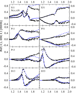
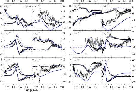
Figure 1: Data SAID for pion-nucleon scattering (l.h.s.) and pion photoproduction (center and r.h.s.) are compared with the results of our calculation. The solid and dashed lines denote the real and imaginary parts of the partial-wave amplitudes, respectively.

IV.1 $\pi+N\to\pi+N$ and $\gamma+p\to\pi+N$

The kernel is chosen similar to what had been used in ref. Kor98 , with the exception of the contact terms for pion photoproduction, which are chosen such that the $\mathsf{A}_{1}^{T}$ and $\mathsf{A}_{2}^{T}$ amplitudes read (only convection current contributions are shown)

$$\mathsf{A}_{1}^{\frac{1}{2}} =\frac{\mathsf{G}_{su}}{s-m^{2}}+\frac{\mathsf{G}_{su}-2\mathsf{G}_{ut}/3}{u-m^{2}}$$ (20)

$$\mathsf{A}_{2}^{\frac{1}{2}} =\frac{2\mathsf{G}_{su}}{(s-m^{2})(u-m^{2})}-\frac{4\mathsf{G}_{ut}/3}{(u-m^{2})(t-m_{\pi}^{2})}$$

$$\mathsf{A}_{1}^{\frac{3}{2}} =\frac{\mathsf{G}_{ut}}{u-m^{2}}$$

$$\mathsf{A}_{2}^{\frac{3}{2}} =\frac{2\mathsf{G}_{ut}}{(u-m^{2})(t-m_{\pi}^{2})}\,,$$

where $G_{su}$ and $G_{ut}$ are defined similar to Eq. (16). This improves the amplitudes at higher energies, while the low-energy behavior is not affected. The results of the calculations are compared with the partial-wave data obtained from the analysis of the Virginia Polytechnic Institute (VPI) group SAID in Fig. 1. The experimental data are reproduced with reasonable accuracy up to the energies of 1.7-1.8 GeV. In the $\pi-N$ sector we attribute the discrepancies at high energies primarily to the inelastic channels not explicitly included in the model. An exception is the $P_{11}$ partial wave, which is traditionally problematic. In our calculation its large width is generated partly due to a large pion-nucleon coupling and partly because of a large decay width to the two-pion production channel.

In the pion photoproduction amplitudes the largest discrepancies are seen in the $\mathsf{M}_{1-}$ and $\mathsf{E}_{2-}$ partial waves for isospin $3/2$. Our investigations show that the $\mathsf{E}_{2-}$ partial wave is almost exclusively sensitive to the $\mathsf{A}_{2}$ contribution, and can be corrected using form factors with cut-off values well below 1 GeV. While this will improve the $\mathsf{E}_{2-}$ partial wave, it also influences strongly all other multipoles and we have chosen not to adapt this procedure for our final calculations. In the case of $\mathsf{M}_{1-}$ partial wave, in addition to the convection current, a number of other sources contribute strongly, such as magnetic terms from the Born contributions and the $\omega$ t-channel. All these contributions are however fixed by their components in other partial waves.

To be able to estimate the effects of the missing inelastic channels on the kaon sector we introduced in the model the $\rho-N$ final state where the coupling is through Born terms only. As expected, its inclusion generates sizable in-elasticities for certain multipoles in the $(N+\pi\to N+\pi)$ sector.

We note, that by fitting the pion scattering and pion photoproduction amplitudes, masses, pion- and photon-coupling constants for the most of the resonances are fixed which strongly limits the number of free parameters for the kaon-production channels.

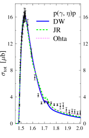
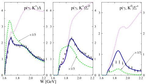
Figure 2: [Color online] Total cross-sections for $\eta$ and kaon photoproduction. Solid line corresponds to the current fit, based on the DW prescription for gauge invariance restoration. Dashed line – same parameters but using a Janssen - Ryckebusch (JR) prescription. Dotted line – same using the Ohta prescription. Note that the JR calculation in kaon sector is scaled down by a factor of 3. The data has been taken from refs. SAPHIR1 ; SAPHIR2 ; SAID ; eta2 .

IV.2 $\gamma+p\to\eta+p$

The data for the ($\gamma+p\to\eta+p$) reaction is taken from the on-line database of the VPI group SAID and from eta2 . Our calculation reproduces the cross-section for this reaction channel rather well, see Fig. 2. As is well known the $S_{11}(1525)$ and $S_{11}(1690)$ resonances give the major contribution to the cross section. In the following section it is shown that re-scattering via the $(\gamma+p\to\eta+p)$ channel influences the kaon production channels. It is worth to note, that the effects due to the different choices for the gauge restoration procedure in the $\eta$-channel are negligible, primarily due to the dominance of the resonance contributions in this channel and the relative weakness of the Born contributions.

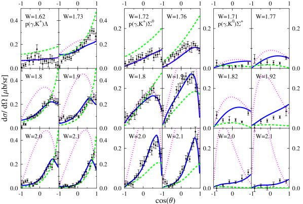
Figure 3: [Color online] Differential cross sections for kaon photoproduction. Line coding is the same as in Fig. 2. The experimental data are from the SAPHIR collaboration SAPHIR1 ; SAPHIR2 .

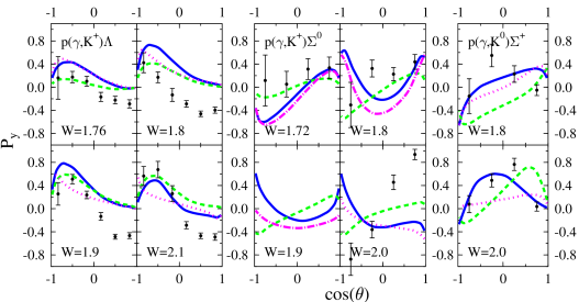
Figure 4: [Color online] Same as Fig. 3 for the final-state polarization in kaon photoproduction.

IV.3 $\gamma+p\to K^{+}+\Lambda$

Our results for photo-induced kaon production are compared to the data from the SAPHIR collaboration SAPHIR1 for angle-integrated cross sections in Fig. 2, for angular distributions in Fig. 3, and for final-state polarization in Fig. 4. The overall agreement with the data is very good, including the asymptotic behavior of the cross-section at high energies. The peaking at 90^∘ seen in the differential cross-section at threshold is not reproduced by our calculation. It should however be noticed that in the CLAS data CLAS1 , see Section IV.5, there is ample evidence for a peaking at 90^∘ at the lowest energies.

The results for the $(\gamma+p\to K+\Lambda)$ cross-sections strongly depend on the choice for the gauge restoration prescription used. In the case of the Ohta prescription the $\mathsf{A}_{2}$ amplitude is unquenched in the high-energy limit, resulting in an unbounded growth of the cross-section. The use of the JR prescription, as compared to the DW, results in a much larger value for the Born contributions. The choice for the gauge restoration procedure is also important for the angular distributions; the use of the JR prescription results in a much more forward-peaked differential cross-section as compared to the prediction following from the DW prescription.

While for the $K+\Lambda$ photoproduction channel it is possible to fit the experimental data using both prescriptions, we prefer the DW prescription for the $K+\Sigma$ photoproduction channel. The couplings extracted using the DW prescription are rather close to the $SU(3)$-model predictions, see Table 3. For the JR prescription we would have to suppress the $g_{N\Lambda K}$ coupling by a factor of $\sqrt{3}$ to compensate the enhancement of the background contributions, which will contradict the predictions of the $SU(3)$ model.

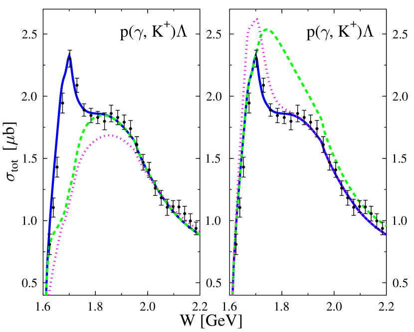
Figure 5: [Color online] Illustration of the re-scattering effects where the solid curve (corresponding to our full calculation) is the same for the left and right panels and serves as a reference. See the text for explanation for the other curves. Note, that the zero point is suppressed in these plots.

The coupled-channel effects are large in the $K-\Lambda$ channel, it not only gives an overall depletion of the cross section at higher energies, but it is responsible for certain structures seen in the spectrum. In particular we find that the narrow structure at 1.7 GeV is generated through re-scattering effects. To illustrate this the results of the following benchmark calculations are compared in Fig. 5.

• The dashed line in the l.h.s. panel corresponds to a calculation in which the photon-nucleon coupling constant for the $S_{11}(1690)$ resonance, $g_{N\gamma}$, is decreased by a factor 10 and the kaon coupling, $g_{K\Lambda}$, increased by the same factor such, that its leading order contribution to the $(\gamma+p\to K+\Lambda)$ reaction remains unchanged. While the full calculation shows the peak at 1.7 GeV, it is missing in the dashed calculation which shows that it is not due to a direct contribution from the resonance, but that re-scattering effects are essential in its formation.

• A detailed investigation at the level of partial wave amplitudes also shows that the peak is due to indirect (coupled-channels) contributions. The direct contribution from the $(\gamma+p\to S_{11}\to K+\Lambda)$ diagram is almost completely cancelled by the corresponding one from the $(\gamma+p\to\pi+N\to S_{11}\to K+\Lambda)$ channel coupling. To illustrate the complicated cancellation we show as the dotted line the results of a calculation where $g_{NK^{*}\Lambda}$ coupling constant is set to zero. Combined with a results of the dashed curve this shows that the dominant contribution to the peak is through the coupled channels contribution $(\gamma+p\to S_{11}\to\pi+N\to K+\Lambda)$, where the $K^{*}$ t-channel contributes to the last step. The direct $K^{*}$ t-channel contribution affects the partial wave amplitudes for $(\gamma+p\to K+\Lambda)$ channel, but the net result on the cross-section is small.

• The dashed line in the r.h.s. panel of Fig. 5 represents the results of a calculation in which the $\rho$-meson final state has been excluded from the model space. The opening of the $\rho$-meson channel takes flux away from the $K\Lambda$-channel thus depleting the cross section near the threshold.

• The dotted line corresponds to a calculation in which the signs of the $\eta$ coupling-constants for both $S_{11}$ resonances have been changed. In leading order this only changes the interference pattern for the $N-\eta$ final state and has no effect on any other channel. As can be seen the effects of channel-coupling are appreciable, even for a rather subtle change in coupling constants in other channels.

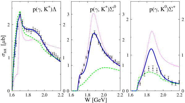
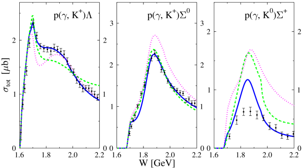
Figure 6: [Color online] The importance of the different contributions for strangeness production is shown. The solid line corresponds to the full calculation. The dashed line in the upper plane corresponds to the calculation where the resonance contributions in the kaon photoproduction channels have been excluded. The dotted line corresponds to the calculation where the channel-coupling effects were switched off. The dashed line in the lower plane corresponds to the calculation, where the $\rho$ t-channel contributions between the different kaon final states were switched off. The dotted line shows the results of a calculation using dipole form-factors Eq. (3) in the u-channel instead of those of Eq. (5).

Our calculations show, as illustrated in Fig. 6, that a major part of the cross-section is generated via non-resonant and re-scattering contributions. Even some prominent structures in the spectrum can be understood as arising through a coupled channels effect. Resonances give only a relatively minor direct contribution to the cross section in the $(\gamma+p\to K+\Lambda)$ channel. The sharp peak in the tree-level calculation corresponds to the second $S_{11}$ resonance and is so prominent due to its small width. In a coupled-channels calculation the width is increased due to the coupling to the $\eta$ channel. The figure shows that for $\Lambda$ production the structure of the u-channel form factor in the strange-sector is not very important. The reason is that the u-channel contribution with an intermediate $\Sigma$ or $\Lambda$-baryon gives only a minor contribution to the cross section. The use of the form factor of Eq. (5) gives rise to a stronger suppression of the u-channel contributions than the usual dipole form Eq. (3), see Fig. 6.

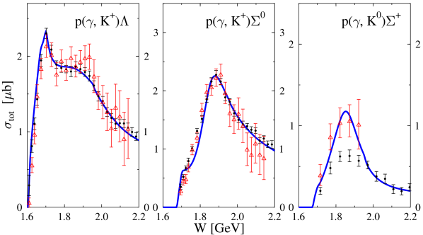
Figure 7: [Color online] Comparison of the old SAPHIR1-old ; SAPHIR2-old and new SAPHIR1 ; SAPHIR2 data for angle integrated cross sections from the SAPHIR Collaboration.

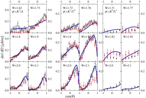
Figure 8: [Color online] Comparison of the old SAPHIR1-old ; SAPHIR2-old and new SAPHIR1 ; SAPHIR2 data for differential cross sections from the SAPHIR Collaboration (triangles).

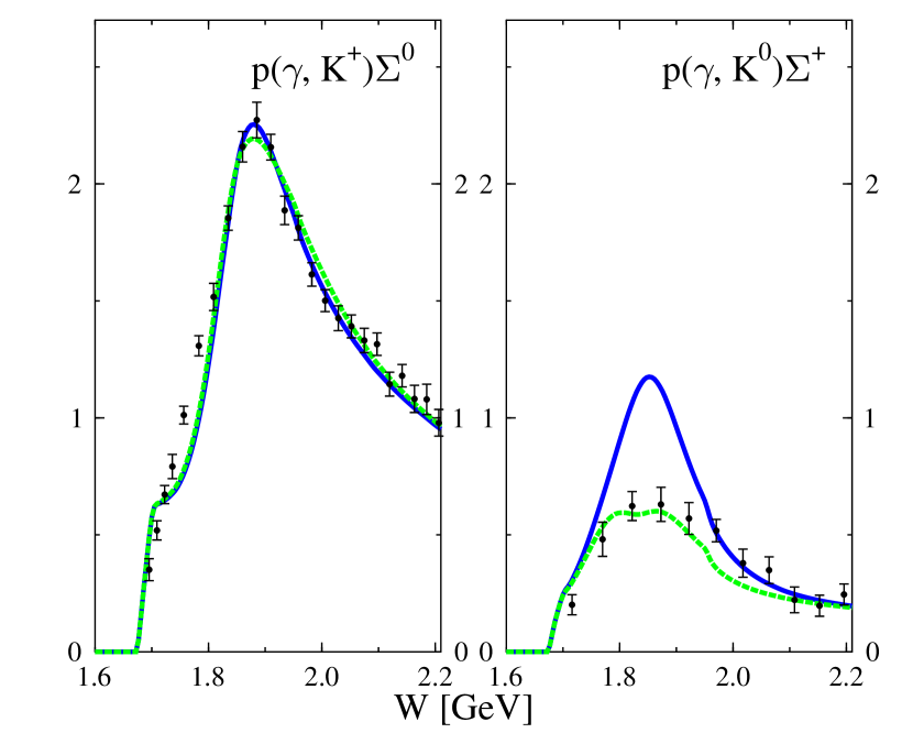
Figure 9: [Color online] Illustration of the effects of the introduction of a second $P_{13}$ resonance.

IV.4 $\gamma+p\to K^{+}+\Sigma^{0}$ and $\gamma+p\to K^{0}+\Sigma^{+}$

The data from two different analyses by the SAPHIR group are compared in Fig. 7 and Fig. 8. While for $\Lambda$- and $\Sigma^{0}$-production the two analyses basically agree, they show big differences for $\Sigma^{+}$-production. The low value for the $\Sigma^{+}$-production cross section poses a problem for the interpretation of the data since the isospin Clebsch-Gordon coefficients are in general larger for $\Sigma^{+}$ than for $\Sigma^{0}$ production. In the $K^{+}\Sigma^{0}$ channel the new data shows a stronger forward peaking of the cross section at high energies than the old.

The difference between the DW and JR prescriptions in the $\Sigma$ channel is even more pronounced than in the $\Lambda$ channel, see Fig. 2 and Fig. 3. The use of the JR prescription results in a larger value for the non-resonant contribution in the $K^{+}\Sigma^{0}$ channel while that for the $K^{0}\Sigma^{+}$ channel is depleted, more in agreement with the new data. However it also predicts a strongly forward-peaked angular distribution in the $\Sigma^{0}$ channel and little forward peaking in the $\Sigma^{+}$ channel, in disagreement with the data.

In the case of the DW prescription the ratio $\Sigma^{0}/\Sigma^{+}$ is much smaller than for JR. To correct for this we introduced modified u-channel form-factors and included $\rho$-meson t-channel contributions. The effects of these contributions is illustrated in the lower plane of Fig. 6. For the dashed line the $\rho$-meson t-channel contribution to the different matrix elements for the kaon states is switched off, which enhances the cross section in $K^{0}\Sigma^{+}$ channel and depletes that for the $K^{+}\Lambda$ channel. The basis for this is a relatively subtle interference between the channels. In obtaining the dotted line the usual dipole form for the u-channel form-factors has been taken. This results in a much larger cross-section especially at higher energies which is in disagreement with the data. The main effect of the use of the form factor Eq. (5) is to suppress the contribution of diagram with a $\Sigma$-baryon in the u-channel and thus suppressing the cross-section at backward angles for $\Sigma^{+}$ production. In the full calculation the cross section at higher energies agrees with the data and shows a gradual decrease at energies beyond those plotted. In $\Sigma^{0}$-production an enhanced cross section at 90^∘ at around 1.9 GeV is observed, which is a strong sign for a $P$ or $D$ resonance, where in the present calculation it is explained via a $P_{33}(1855)$ contribution. However, since such a resonance also contributes strongly to the $K^{0}\Sigma^{+}$ channel, due to isospin symmetry, it needs to be compensated there through the introduction of an additional $P_{13}$ resonance at a similar energy. With the correct couplings the two resonances will interfere constructively in the $K^{+}\Sigma^{0}$ channel and destructively in the $K^{0}\Sigma^{+}$ channel. To illustrate this point the results of a calculation is shown in the Fig. 9, in which a $P_{13}$ resonance is included at $m_{P_{13}}=1830$ MeV with a coupling strength of $g_{{P_{13}}K\Sigma}=0.05$ and width of $W_{P_{33}}=0.10$ GeV, at the same time increasing the width of ${P_{33}}$ to $W_{P_{33}}=0.25$ (using the same photon couplings as shown in Table 1 for both of them). Shown are total cross-sections for $K^{0}\Sigma^{+}$ and $K^{+}\Sigma^{0}$ channels. The angular distributions for the $K^{+}\Sigma^{0}$ channel are also improved, while those for $K^{0}\Sigma^{+}$ are not affected. The rest of observables (including final-state polarization) are not modified or modified only slightly.

Compared to the $K^{+}\Lambda$ channel the resonances play a larger role in the $\Sigma$ channels, especially in the $K^{+}\Sigma^{0}$. At the same time we have found the inclusion of the coupled-channels effects to play an important role, as it suppresses the cross-section at the higher energies.

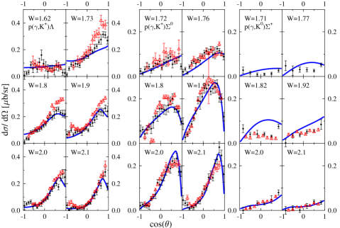
Figure 10: [Color online] Comparison of our calculation with the new data from the SAPHIR Collaboration SAPHIR1 ; SAPHIR2 (circles) and the data from the CLAS collaboration CLAS1 ; CLAS2 (triangles).

IV.5 Comparison with the CLAS data

In Fig. 10 the new SAPHIR data SAPHIR1 ; SAPHIR2 is compared to the data from the CLAS collaboration CLAS1 ; CLAS2 . From this figure we can see that the two data sets agree in overall magnitude but do show some important differences.

In the $K^{+}\Lambda$ channel the most important difference between the two data sets is the cross-section at the very forward angles. For the SAPHIR data, the cross-section clearly drops off, while this is not seen in the CLAS data. As it was noted before, the trend at forward angles is very sensitive to the gauge restoration scheme chosen. An alternative way to account for this difference will be the inclusion of the $K_{1}$ t-channel contribution Ire04 , which is not needed for the SAPHIR data. Another difference lies at backward angles where the CLAS data at 1.9 GeV and 2.1 GeV show a much more pronounced peak in the angular distribution. Our calculation does not reproduce this peak, but it could possibly be the indication for an additional $P$ or $D$ resonance.

In the $K^{+}\Sigma^{0}$ channel the difference between the two data sets is that in the CLAS data the bump in the cross section at 90^∘ is slightly more pronounced than in the CLAS data.

V Conclusions

In this work we showed that for a calculation of meson production at higher energies, in particular kaon production, it is essential to perform a full coupled channels calculation. The effects of channel coupling are not just a smooth change of the energy dependence of the cross section, but can also give rise to structures in the cross section which might otherwise be misinterpreted as resonances.

An additional advantage of a full coupled channels calculation is that it allows for a simultaneous calculation of observables for a large multitude of reactions with considerably fewer parameters than would be necessary if each reaction channel would be fitted separately. As shown the coupled-channels calculation is manageable if the K-matrix formalism is used.

For photoproduction reactions it is necessary to perform a gauge-invariant calculation. The particularities of the gauge restoration procedure are however model dependent. For low photon energies this model dependence does not reflect strongly on observables. At higher photon energies ($\omega$), corresponding to the threshold of kaon production and beyond, the model dependencies in gauge-restoration procedures give rise to strongly different Born contribution to the amplitude and result in large differences in extracted coupling parameters or predictions for cross sections that are at variance with the data. The reason for this is that the differences between the various gauge-restoration procedures are of higher order in $\omega$ which gives rise to large terms when $\omega/m\approx 1$. The observables are thus sensitive to short-range effects and one is entering the energy regime where quark effects will start to be important.

The calculations presented in this work show that a good fit to the data can be obtained using the DW prescription for the gauge restoration terms. The model parameters were fitted to the data and are largely consistent with SU(3). Some notable differences from SU(3) and some discrepancies in reproducing the data could be attributed to the need for a second $P_{13}$ resonance at an energy of around 1.9 GeV.

Appendix A Lagrangian

In this section we present the effective-field Lagrangian used in this work. A comparison is presented with $SU(3)$ predictions of the model parameters and their values as extracted from our fit. A summary of the $SU(3)$ notation used is presented in Appendix B.

The $SU(3)$-model predictions for the coupling constants of baryons have a long history dating back to the papers by Rijken and de Swart Swa79 , where they found $F/D\simeq 0.69$. In ref. Swa89 a value of $F/D\simeq 0.55$ was found. In ref. Bor99 a recent calculation is presented on the extraction of $SU(3)$-model parameters from semi-leptonic decays $B\to B^{\prime}+e^{-}+\bar{\nu}_{e}$. The extracted values range from $F/D\simeq 0.84$ down to $F/D\simeq 0.59$. A calculation based on QCD sum rules Kim00 arrived at a rather small value $F/D\simeq 0.2$. The values of the couplings constants obtained with $F/D=0.55$ in the extreme quark model ($S=3F-D$) are presented in a Table 3 (BBP, upper plane) and agree very well with the values we obtained from our fit with the only notable exception of $g_{N\Sigma K}$. The $SU(3)$ prediction for this coupling constant is very sensitive to the exact value of $F/D$ and our extracted values can be seen as an argument to favor a somewhat smaller value for $F/D$. We should note that the relative sign of the $g_{N\Sigma K}$ and $g_{N\Lambda K}$ couplings is often taken to be negative Cot04 . It should be noted, however, that this sign cannot be determined from a calculation as presented in this work because it depends on an arbitrary sign in the definition of the $\Lambda$-baryonic field. In weak-decay processes the sign of the vector v.s. axial vector can be determined, which only fixes the sign of the axial coupling if the vector coupling is assumed to be positive Cot04 .

For the Baryon-Baryon-Vector (BBV, Table 3, lower plane) sector the $SU(3)$ predictions are based on the assumptions of the extreme quark model and vector meson universality Swa89 , which requires $S=3F-D$ and $D=0$. With this choice for $SU(3)$ parameters the agreement between $SU(3)$ predictions and values extracted from our calculation is reasonable with the exception of the $\rho\Sigma\Sigma$ and $\rho\Sigma\Lambda$ couplings which are extracted to be much larger. A reason for this could be that in the present calculation, in order to limit the number of free parameters, the magnetic coupling of the $\rho$-meson, $\kappa_{\rho}$ was kept fixed for the different baryons.

Table 3: Baryon-meson summary table, defining $\Gamma(X)=(\chi X+i\gamma_{\mu}\partial^{\mu}X/2M)/(\chi+1)\gamma_{5}$ and $\Gamma^{\prime}(X)=\gamma_{\mu}X^{\mu}+\frac{\kappa_{X}}{2M}(\sigma_{\mu\nu}\partial^{\nu}X^{\mu})$.

$\mathcal{L}$	$SU(3)$	$g_{SU(3)}$	$g_{\text{model}}$
$BBP$
$ig_{NN\pi}\bar{N}\Gamma(\vec{\pi}\cdot\vec{\tau})N$	$(D+F)/\sqrt{2}$	$13.47$	$13.47$
$ig_{NN\eta}\bar{N}\Gamma(\eta)N$	$(2S+3F-D)/3\sqrt{2}$	$5.6$	$3.0$
$ig_{N\Lambda\mathsf{K}}\bar{\Lambda}\Gamma(\bar{}\mathsf{K})N$	$(D+3F)/\sqrt{6}$	$13.3$	$12$
$ig_{N\Sigma\mathsf{K}}\bar{\Sigma}_{i}\Gamma(\bar{}\mathsf{K}\tau_{i})N$	$(D-F)/\sqrt{2}$	$3.9$	$8.6$
$BBV$
$-g_{NN\rho}\bar{N}\Gamma^{\prime}(\vec{\rho}\cdot\vec{\tau})N$	$(D+F)/\sqrt{2}$	$2.2$	$2.2$
$-g_{NN\omega}\bar{N}\Gamma^{\prime}(\omega)N$	$(2S+3F-D)/3\sqrt{2}$	$6.6$	$8$
$-g_{NN\phi}\bar{N}\Gamma^{\prime}(\phi)N$	$(3F-D-S)/3$	$0$	$0$
$-g_{N\Lambda K^{*}}\bar{\Lambda}\Gamma^{\prime}(\bar{}\mathsf{K}^{*})N$	$(D+3F)/\sqrt{6}$	$3.8$	$1.7$
$-g_{N\Sigma K^{*}}\bar{\Sigma}_{i}\Gamma^{\prime}(\bar{}\mathsf{K}^{*})\tau_{i}N$	$(D-F)/\sqrt{2}$	$-2.2$	$0$
$-g_{\Sigma\Sigma\rho}\varepsilon_{ijk}\bar{\Sigma}_{i}\Gamma^{\prime}(\rho_{j})\Sigma_{k}$	$F\sqrt{2}$	$4.4$	$10$
$-g_{\Sigma\Lambda\rho}\bar{\Sigma}_{i}\Gamma^{\prime}(\rho_{i})\Lambda$	$-D\sqrt{2/3}$	$0$	$-10$

The values for the baryon magnetic moments as used in the calculation are summarized in Table 4 and are taken to agree with those quoted by the Particle Data Group PDG . The value for $\kappa_{\Sigma^{0}}$ is taken from the quark model prediction Perkins . The $SU(3)$ parameters used are $\kappa_{F}=0.83$ and $\kappa_{D}=2.86$. Note that the sign of the transition moment, $\kappa_{\Lambda\Sigma}$, is chosen to agree with the $SU(3)$ prediction.

Table 4: Baryon-photon summary table.

Vertex	$SU(3)$	$g_{SU(3)}$	$g_{\text{model}}$
$\kappa_{p}$	$\kappa_{F}+\kappa_{D}/3$	$1.783$	$1.79$
$\kappa_{n}$	$-2\kappa_{D}/3$	$-1.907$	$-1.91$
$\kappa_{\Sigma^{+}}$	$\kappa_{F}+\kappa_{D}/3$	$1.783$	$1.45$
$\kappa_{\Sigma^{-}}$	$-\kappa_{F}+\kappa_{D}/3$	$0.123$	$-0.16$
$\kappa_{\Sigma^{0}}$	$\kappa_{D}/3$	$0.953$	$0.79$
$\kappa_{\Lambda}$	$-\kappa_{D}/3$	$-0.953$	$-0.613$
$\kappa_{\Lambda\Sigma}$	$-\kappa_{D}/\sqrt{3}$	$-1.651$	$-1.61$

Table 5 summarizes the couplings in the meson sector, in particular those for the Vector-Pseudoscalar-Pseudoscalar (VPP, upper plane) and Vector-Pseudoscalar-Photon (VPA, lower plane) interaction Lagrangians. For these sectors there are experimental data for meson decay widths PDG , which allows for the extraction of absolute magnitudes of coupling constants. For the $SU(3)$ parameters we have chosen to adapt the predictions of the extreme quark model, which dictates $G_{18}=\sqrt{2}G_{88}$ for VPA and $G_{81}=0$ for the VPP sectors of the model. As can be seen from the magnitude of the $\phi\pi\gamma$ coupling constant, this does not hold exactly but to a good extent. The parameters in our calculation were fixed to the values extracted from decay data where available, or to the $SU(3)$ predictions otherwise. The same holds for the $\pi\gamma\gamma$ and $\eta\gamma\gamma$ coupling constants.

Table 5: Meson summary table, defining $\varepsilon(ABCD)=(\varepsilon_{\mu\nu\rho\sigma}(A^{\rho}B^{\mu})(C^{\sigma}D^{\nu}))$

$\mathcal{L}$	$SU(3)$	$g_{SU(3)}$	$|g_{\text{decay}}|$	$g_{\text{model}}$
$VPP$
$-ig_{\phi\mathsf{K}\mathsf{K}}\bar{}\mathsf{K}\tensor{\partial}^{\mu}\mathsf{K}\phi_{\mu}$	$-G_{88}$	$-4.5$	$\begin{cases}4.48\pm 0.07,K^{\pm}\\ 4.60\pm 0.08,K^{0}\end{cases}$	$-4.5$
$-ig_{\eta\mathsf{K}\mathsf{K}^{*}}\mathsf{K}\tensor{\partial}^{\mu}\eta\bar{}\mathsf{K}^{*}_{\mu}$	$G_{88}/\sqrt{2}-G_{81}\sqrt{2}$	$3.2$		$-3.2$
$-ig_{\pi\mathsf{K}\mathsf{K}^{*}}\bar{}\mathsf{K}\tensor{\partial}^{\mu}\vec{\pi}\cdot\vec{\tau}\mathsf{K}^{*}_{\mu}$	$G_{88}/\sqrt{2}$	$3.2$	$3.26\pm 0.03$	$-3.26$
$-ig_{\rho\mathsf{K}\mathsf{K}}\bar{}\mathsf{K}\tensor{\partial}^{\mu}\tau_{i}\mathsf{K}\rho_{i\mu}$	$-G_{88}/\sqrt{2}$	$-3.2$		$-3$
$-ig_{\rho\pi\eta}(\eta\tensor{\partial}^{\mu}\vec{\pi})\cdot\vec{\rho}_{\mu}$	$-G_{81}\sqrt{2}$	$0$	$<2.7$	$0$
$-ig_{\rho\pi\pi}\varepsilon_{ijk}{\vec{\rho}_{i\mu}}{(\vec{\pi}_{j}\tensor{\partial}^{\mu}\vec{\pi}_{k})}/2$	$G_{88}\sqrt{2}$	$6.36$	$6.00\pm 0.06$	$6.0$
$VPA$
$\frac{g_{\rho\gamma\pi}}{m_{\pi}}\vec{\pi}^{0}\cdot\varepsilon(\partial A\partial\vec{\rho})$	$G_{88}/3$	$-0.11$	$0.12\pm 0.02$	$-0.12$
$\frac{g_{\rho\gamma\pi}}{m_{\pi}}\vec{\pi}^{\pm}\cdot\varepsilon(\partial A\partial\vec{\rho})$	$G_{88}/3$	$-0.11$	$0.101\pm 0.006$	$-0.10$
$\frac{g_{\omega\gamma\pi}}{m_{\pi}}\pi^{0}\varepsilon(\partial A\partial\omega)$	$(G_{88}+G_{18}\sqrt{2})/3$	$-0.33$	$0.322\pm 0.007$	$0.32$
$\frac{g_{\phi\gamma\pi}}{m_{\pi}}\pi^{0}\varepsilon(\partial A\partial\phi)$	$(G_{88}\sqrt{2}-G_{18})/3$	$0.0$	$0.018\pm 0.001$	$0.018$
$\frac{g_{\phi\gamma\eta}}{m_{\pi}}\eta\varepsilon(\partial A\partial\phi)$	$(2G_{81}-G_{18}-G_{88}\sqrt{2})/9$	$0.1$	$0.096\pm 0.002$	$0.096$
$\frac{g_{\mathsf{K}^{*}\mathsf{K}\gamma}}{m_{\pi}}\bar{}\mathsf{K}^{0}\varepsilon(\partial A\partial\mathsf{K}^{*})$	$-2G_{88}/3$	$0.22$	$0.177\pm 0.009$	$-0.177$
$\frac{g_{\mathsf{K}^{*}\mathsf{K}\gamma}}{m_{\pi}}\bar{}\mathsf{K}^{\pm}\varepsilon(\partial A\partial\mathsf{K}^{*})$	$G_{88}/3$	$-0.11$	$0.117\pm 0.007$	$0.117$

Appendix B $SU(3)$ notation

The notation used to derive the $SU(3)$ model couplings is summarized. Our notation agrees with that of ref. Tit99 , and a more detailed review of $SU(3)$ can be found in ref. Swa63 or ref. Mos89 .

The definition for pseudo-scalar singlet is

$$P_{1}=\operatorname{diag}(1,1,1)\eta_{1}\,,$$ (21)

and that for the octet

$$P_{8}=\begin{pmatrix}\displaystyle\frac{\pi^{0}}{\sqrt{2}}+\frac{\eta_{8}}{\sqrt{6}}&\pi^{+}&K^{+}\\ \pi^{-}&-\displaystyle\frac{\pi^{0}}{\sqrt{2}}+\frac{\eta_{8}}{\sqrt{6}}&K^{0}\\ K^{-}&\bar{K}^{0}&-2\eta_{8}/\sqrt{6}\end{pmatrix}\,,$$ (22)

where in the quark model $\pi^{0}=(u\bar{u}-d\bar{d})/\sqrt{2}$, $\eta_{1}=(u\bar{u}+d\bar{d}+s\bar{s})/\sqrt{3}$, and $\eta_{8}=(u\bar{u}+d\bar{d}-2s\bar{s})/\sqrt{6}$. The photon field couples to the charge, which in SU(3) language is

$$\hat{Q}=\operatorname{diag}(2/3,-1/3,-1/3)\;.$$ (23)

The baryon octet is given by

$$\begin{split}B_{8}&=\begin{pmatrix}\displaystyle\frac{\Sigma^{0}}{\sqrt{2}}-\frac{\Lambda}{\sqrt{6}}&\Sigma^{+}&p\\ \Sigma^{-}&-\displaystyle\frac{\Sigma^{0}}{\sqrt{2}}-\frac{\Lambda}{\sqrt{6}}&n\\ \Xi^{-}&\Xi^{0}&+2\Lambda/\sqrt{6}\end{pmatrix}\\ &=\begin{pmatrix}uds&uus&uud\\ dds&uds&udd\\ dss&uss&uds\end{pmatrix}\,.\end{split}$$ (24)

The Lagrangian for the different $SU(3)$ sectors read

$$\mathcal{L}_{VPP} =G_{88}\operatorname{Tr}\Big{[}V_{8}^{\mu}(P_{8}\cdot\partial_{\mu}P_{8}-\partial_{\mu}P_{8}\cdot P_{8})\Big{]}$$ (25)

$$\quad+G_{81}\sqrt{3}\operatorname{Tr}\Big{[}V_{8}^{\mu}(P_{8}\cdot\tensor{\partial}_{\mu}p_{1})\Big{]}$$

$$\mathcal{L}_{VPA} =i\varepsilon_{\mu\nu\alpha\beta}k_{V}^{\alpha}(\partial^{\mu}A^{\nu})\Biggl{[}G_{81}\sqrt{\frac{2}{3}}\operatorname{Tr}\Big{[}\hat{Q}V_{8}^{\beta}P_{1}\Big{]}$$ (26)

$$+G_{18}\sqrt{\frac{2}{3}}\operatorname{Tr}\Big{[}\hat{Q}V_{1}^{\beta}P_{8}\Big{]}+G_{88}\operatorname{Tr}\Big{[}\hat{Q}\big{\{}V_{8}^{\beta},P_{8}\big{\}}_{+}\Big{]}\Biggr{]}$$

$$\mathcal{L}_{BBP} =D\operatorname{Tr}\Big{[}P_{8}\{B_{8},\bar{B}_{8}\}_{+}\Big{]}$$ (27)

$$\quad+F\operatorname{Tr}\Big{[}P_{8}[B_{8},\bar{B}_{8}]_{-}\Big{]}+\frac{S}{\sqrt{3}}\operatorname{Tr}\Big{[}P_{1}\bar{B}_{8}B_{8}\Big{]}$$

The physical particles are related to the pure octet and singlet states as

$$\begin{split}\eta=&\eta_{8}\cos\theta_{P}+\eta_{1}\sin\theta_{P}\\ &\approx(\eta_{8}+\sqrt{2}\eta_{1})/\sqrt{3}=(u\bar{u}+d\bar{d})/\sqrt{2}\\ \eta^{\prime}=&\eta_{8}\sin\theta_{P}-\eta_{1}\cos\theta_{P}\\ &\approx(\sqrt{2}\eta_{8}-\eta_{1})/\sqrt{3}=-s\bar{s}\end{split}$$ (28)

for $\theta_{P}=60^{\circ}-\Delta\theta_{P}$. For vector particles, $V$ (scalar, $S$) similar definitions apply replacing only $\pi\to\rho(a_{0})$, $\eta\to\omega(\sigma)$, $\eta^{\prime}\to\Phi(f_{0})$, $K\to K^{*}(K^{*}_{0})$.

References

- (1) U. Löring, K. Kretzschmar, B.Ch. Metsch and H.R. Petry, Eur. Phys. J. A 10, 309 (2001); U. Löring, B.Ch. Metsch and H.R. Petry, Eur. Phys. J. A 10, 395 (2001); 10, 447 (2001).
- (2) L. Theußl, R.F. Wagenbrunn, B. Desplanques, and W. Plessas, Eur. Phys. J. A 12, 91 (2001).
- (3) G. Penner and U. Mosel, Phys. Rev. C 66, 055211 (2002); 66, 055212 (2002).
- (4) R.M. Davidson and R. Workman, Phys. Rev. C 63, 025210 (2001).
- (5) K. Ohta, Phys. Rev. C 40, 1335 (1989).
- (6) A.I. Titov and T.-S. H. Lee, Phys. Rev. C 66, 015204 (2002); 67, 065205 (2003).
- (7) D.G. Ireland, S. Janssen and J. Ryckebusch, Nucl. Phys. A 740, 147 (2004).
- (8) S. Janssen, J. Ryckebusch, D. Debruyne, and T. Van Cauteren, Phys. Rev. C 66, 035202 (2002).
- (9) F.X. Lee, T. Mart, C. Bennhold, H. Haberzettl and L.E. Wright, Nucl. Phys. A 695, 237 (2001).
- (10) V. Bernard, N. Kaiser and U.-G. Meißner, Int. J. Mod. Phys. E 4, 193 (1995).
- (11) K.-H. Glander et al. (SAPHIR Collaboration), Eur. Phys. J. A 19, 251 (2004).
- (12) R. Lawall et al. (SAPHIR Collaboration),, Eur. Phys. J. A 24, 275 (2005)
- (13) A.Yu. Korchin, O. Scholten and R.G.E. Timmermans, Phys. Lett. B 438, 1 (1998).
- (14) O. Scholten, S. Kondratyuk, L. Van Daele, D. Van Neck, M. Waroquier and A.Yu. Korchin, Acta Phys. Pol. B33, 847 (2002).
- (15) R.G. Newton, Scattering theory of Waves and Particles (Springer, New York, 1982).
- (16) S. Kondratyuk and O. Scholten, Nucl. Phys. A 677, 396 (2000); Phys. Rev. C 62, 025203 (2000).
- (17) S. Kondratyuk and O. Scholten, Phys. Rev. C 65, 038201 (2002); 64, 024005 (2001).
- (18) A.Yu. Korchin and O. Scholten, Phys. Rev. C 68, 045206 (2003).
- (19) T. Sato and T.-S.H. Lee, Phys. Rev. C 54, 2660 (1996).
- (20) W.T. Chiang, B. Saghai, F. Tabakin, T.-S.H. Lee, Phys. Rev. C 69, 65208 (2004).
- (21) M.F.M. Lutz and E.E. Kolomeitsev, Nucl. Phys. A 700, 193 (2002).
- (22) S. Kondratyuk, K. Kubodera, F. Myhrer and O. Scholten, Nucl. Phys. A 736, 339 (2004).
- (23) V. Shklyar, G. Penner and U. Mosel, Eur. Phys. J. A 21, 2004 (445).
- (24) V. Pascalutsa, Nucl. Phys. A 680, 76 (2000).
- (25) V. Pascalutsa, Phys. Lett. B 503, 85 (2001).
- (26) Particle Data Group, K. Hagiwara et al., Phys. Rev. D 66, 010001 (2002).
- (27) I.J. General and S.R. Cotanch, Phys. Rev. C 69, 035202 (2004)
- (28) S. Janssen, private communications.
- (29) R.A. Arndt, I.I. Strakovsky and R.L. Workman, Phys. Rev. C 53, 430 (1996); 66, 055213 (2002); updates available on the web: http://gwdac.phys.gwu.edu.
- (30) V. Crede et al. (CB-ELSA Collaboration), Phys. Rev. Lett. 94, 012004 (2005).
- (31) J.W.C. McNabb et al. (CLAS Collaboration), Phys. Rev. C 69, 042201 (2004).
- (32) M.Q. Tran et al. (The SAPHIR Collaboration), Phys. Lett. B 445, 20 (1998).
- (33) S. Goers et al. (The SAPHIR Collaboration), Phys. Lett. B 464, 331 (1999).
- (34) B. Carnahan, Ph.D. thesis, CUA, 2003.
- (35) M.N. Nagels, T.A. Rijken, and J.J. de Swart, Phys. Rev. D 20, 1633 (1979).
- (36) P.M.M. Maessen, Th.A. Rijken, and J.J. de Swart, Phys. Rev. C 40, 2226 (1989).
- (37) B. Borasoy, Phys. Rev. D 59, 054021 (1999).
- (38) H. Kim, T. Doi, M. Oka and S.H. Lee, Nucl. Phys. A 662, 371 (2000)
- (39) D.H. Perkins, Introduction to High Energy Physics, 4th ed. (Cambridge University Press, Cambridge, 2000).
- (40) A.I. Titov et al., Phys. Rev. C 60, 035205 (1999).
- (41) J.J. de Swart, Rev. Mod. Phys. 35, 916 (1963).
- (42) Ulrich Mosel, Fields, Symmetries, and Quarks (McGraw-Hill, 1989).