The sigma - nucleon form factor in a chiral topological model with anomalous dimension.

Abstract

The chiral soliton model including $\pi,\rho,\omega$ mesons is extended for the case when the scalar - isoscalar $\sigma$ meson has an anomalous dimension - d. The form factor of the sigma - nucleon interaction calculated and to be found not highly sensitive to the value of d.

I Introduction

It is well known that, the scalar isoscalar $\sigma$-meson plays an important role in nucleon - nucleon (NN) interaction. In one boson exchange model (OBE) of NN interaction one has to take into account the form - factor of $\sigma NN$ vertex which is still poorly known. In our recent paper [1] we considered the form - factor in the framework of $\pi\rho\omega\sigma$ soliton model including a dilaton field as a sigma meson with the ordinary scale dimension $d=1$. On the other hand, there are some versions of chiral effective Lagrangians for the finite nuclear matter and finite nuclei where light scalar degrees of freedom have an anomalous scale dimension [2].

Note that, anomalous, fractal, scale dimensions are ingredient feature of modern theories. In particular it has been recently shown that, fractal scale dimension is essential to describe superconductivity [3]. In present brief note we study the role of anomalous scale dimension in $\sigma NN$ interaction. The paper is organized as follows. In Sect. II we outline the scaling prpoperties of basic fields; in Sect. III we shall extend the $\pi,\rho,\omega$ Lagrangian for the case of anomalous dimension; in Sect. IV we calculate the vertex form factor of $\sigma N$ interaction. The results and brief summary are presented in Sect. V

II Scaling behavior of scalar and spinor fields

In this section, to make the point clearer and for further references we briefly discuss the scaling properties of various fields. For illustration we consider kinetic terms of fermion and boson fields. The kinetic terms of a fermion field (e.g. quark field in QCD, or nucleon field) is given by

$${\cal{L}}_{{\displaystyle\mbox{kin}}}^{\psi}(x)=i\bar{\psi}(x)\partial^{\mu}\gamma_{\mu}\psi(x)$$ (1)

and a boson ($\pi$ or $\sigma$) field

$${\cal{L}}_{{\displaystyle\mbox{kin}}}^{\pi}(r)=\displaystyle\frac{1}{2}\partial_{\mu}\pi\partial^{\mu}\pi.$$ (2)

The scale invariance demands that the action $S=\int d^{4}x\cal L$ should be invariant under scale transformations $x_{\mu}={e}^{\displaystyle{-\lambda}}{x}^{\prime}_{\mu}:$

$$S=\int d^{4}x{\cal{L}}_{{\displaystyle\mbox{kin}}}(x)=\int d^{4}{x}^{\prime}{\cal{L}}_{{\displaystyle\mbox{kin}}}^{\prime}({x}^{\prime})$$ (3)

Let the fermion and boson fields scale as $\psi(x)=\exp{(n\lambda)}\psi^{\prime}({x}^{\prime})$ and $\pi(x)=\exp{(m\lambda)}\pi^{\prime}({x}^{\prime}),$ respectively. For fermions we get

$$\begin{array}[]{l}S=i\displaystyle\int d^{4}x\bar{\psi}(x)\partial^{\mu}\gamma_{\mu}\psi(x)=i\displaystyle\int d^{4}{x}^{\prime}\bar{\psi}^{\prime}({x}^{\prime})\partial^{\mu}\gamma_{\mu}\psi^{\prime}({x}^{\prime}){e}^{\displaystyle{\lambda}}{e}^{\displaystyle{2n\lambda}}{e}^{\displaystyle{-4\lambda}}=\\[5.69054pt] =\displaystyle\int d^{4}{x}^{\prime}{\cal{L}}_{{\displaystyle\mbox{kin}}}^{\prime}({x}^{\prime})\end{array}$$ (4)

and hence $-4\lambda+\lambda+2n\lambda=\lambda(2n-3)=0$. Since $\lambda$ is arbitrary then $n=3/2$. Similarly, for boson fields one can show that $m=1$. Therefore we may conclude that

$$x_{\mu}\rightarrow{e}^{\displaystyle{-\lambda}}x_{\mu},\quad\psi(x)\rightarrow{e}^{\displaystyle{3\lambda/2}}\psi(x),\quad\pi(x)\rightarrow{e}^{\displaystyle{\lambda}}\pi(x)\,,$$ (5)

i.e. the scale dimension $d$ equals to $d_{f}=3/2$ and $d_{b}=1$ for fermions and bosons respectively. Thus, the term ”anomalous scale dimension” e.g. for a boson field means $d_{b}\neq 1$.

In Skyrme like models the pion field is involved through a chiral nonlinear field $U=\exp{(i\vec{\tau}\cdot\vec{\pi}/f_{\pi})}$ which has trivial scale dimension $d_{U}=0$. For this reason the four derivative term of the Skyrme Lagrangian given by

$${\cal{L}}_{\mbox{4}}=\displaystyle\frac{1}{32e^{2}}\mbox{Tr\,}[(\partial_{\mu}U)U^{+},(\partial_{\nu}U)U^{+}]^{2}$$ (6)

is scale invariant by itself:

$$\int d^{4}x{\cal{L}}_{\mbox{4}}(x)\rightarrow\int d^{4}{x}^{\prime}{e}^{\displaystyle{-4\lambda}}{\cal{L}}_{\mbox{4}}^{\prime}({x}^{\prime}){e}^{\displaystyle{4\lambda}}=\int d^{4}{x}^{\prime}{\cal{L}}_{\mbox{4}}^{\prime}({x}^{\prime})\,,$$ (7)

whereas the kinetic term

$${\cal{L}}_{\mbox{2}}(x)=\displaystyle\frac{f_{\pi}^{2}}{4}\mbox{Tr\,}[\partial_{\mu}U(x)\partial^{\mu}U^{+}(x)]$$ (8)

is not:

$$\begin{array}[]{l}\displaystyle\int d^{4}x{\cal{L}}_{\mbox{2}}(x)\rightarrow\displaystyle\frac{f_{\pi}^{2}}{4}\displaystyle\int d^{4}{x}^{\prime}{e}^{\displaystyle{-4\lambda}}{e}^{\displaystyle{2\lambda}}\mbox{Tr\,}[\partial_{\mu}U^{\prime}({x}^{\prime})\partial^{\mu}U^{{}^{\prime}+}({x}^{\prime})]=\\[5.69054pt] ={e}^{\displaystyle{-2\lambda}}\displaystyle\int d^{4}{x}^{\prime}{\cal{L}}_{\mbox{2}}^{\prime}({x}^{\prime})\end{array}$$ (9)

How can the invariance be restored? According to Shehter [4] an additional boson field $\chi(x)$ should be included into the Skyrme Lagrangian. We shall use this prescription in the next Section.

III The $\pi\rho\omega\sigma$ model with anomalous dimension

We start with extended Skyrme - like Lagrangian including vector mesons explicitely [5]

$$\begin{array}[]{l}{\cal{L}}=-\displaystyle\frac{f_{\pi}^{2}}{4}\mbox{Tr\,}L_{\mu}L^{\mu}-\displaystyle\frac{f_{\pi}^{2}}{2}\mbox{Tr\,}[l_{\mu}+r_{\mu}+ig\vec{\tau}\vec{\rho}_{\mu}+ig\omega_{\mu}]^{2}+\displaystyle\frac{3}{2}g\omega_{\mu}B^{\mu}-\displaystyle\frac{1}{4}(\omega_{\mu\nu}\omega^{\mu\nu}+\vec{\rho}_{\mu\nu}\vec{\rho}^{\,\,\mu\nu})\\[5.69054pt] \\ \quad\quad+\displaystyle\frac{f_{\pi}^{2}m_{\pi}^{2}}{2}\mbox{Tr\,}(U-1)\,,\end{array}$$ (10)

where left/right–handed currents are given by $L_{\mu}=U^{+}\partial_{\mu}U$, $l_{\mu}=\xi^{+}\partial_{\mu}\xi$, $r_{\mu}=\xi\partial_{\mu}\xi^{+}$,$\quad\xi=\sqrt{U}$, and the pertinent vector meson ($\vec{\rho},\omega$) field strength tensors are $\vec{\rho}_{\mu\nu}=\partial_{\mu}\vec{\rho}_{\nu}-\partial_{\nu}\vec{\rho}_{\mu}+g[\vec{\rho}_{\mu}\times\vec{\rho}_{\nu}]$ and $\omega_{\mu\nu}=\partial_{\mu}\omega_{\nu}-\partial_{\nu}\omega_{\mu}$. Furthermore, the topological baryon number current is given by $B^{\mu}=\varepsilon^{\mu\alpha\beta\gamma}\mbox{Tr\,}L_{\alpha}L_{\beta}L_{\gamma}/(24\pi^{2})$. Note that, for the case of infinite $\rho$ and $\omega$ meson masses the Lagrangian in Eq. (10) becomes equal to the usual Skyrme -Witten Lagrangian with two, four and six derivative terms and, hence, is not scale invariant. As it has been mentioned above this shortcoming can be restored by inclusion of a dilaton field - sigma meson. Thus, including a $\sigma$–meson by means of the scale invariance and trace anomaly of QCD into the Lagrangian one obtains following chiral Lagrangian of the coupled $\pi\rho\omega\sigma$ system

$$\begin{array}[]{l}{\cal{L}}=\displaystyle\frac{S_{0}^{2}e^{-2\sigma/d}}{2}\partial_{\mu}\sigma\partial^{\mu}\sigma-\displaystyle\frac{f_{\pi}^{2}e^{-2\sigma/d}}{4}\mbox{Tr\,}L_{\mu}L^{\mu}-\displaystyle\frac{f_{\pi}^{2}e^{-2\sigma/d}}{2}\mbox{Tr\,}[l_{\mu}+r_{\mu}+ig\vec{\tau}\vec{\rho}_{\mu}+\\[5.69054pt] \\ +ig\omega_{\mu}]^{2}+\displaystyle\frac{3}{2}g\omega_{\mu}B^{\mu}-\displaystyle\frac{1}{4}(\omega_{\mu\nu}\omega^{\mu\nu}+\vec{\rho}_{\mu\nu}\vec{\rho}^{\,\,\mu\nu})+\displaystyle\frac{f_{\pi}^{2}m_{\pi}^{2}e^{-3\sigma/d}}{2}\mbox{Tr\,}(U-1)-\\[5.69054pt] \\ -\displaystyle\frac{d^{2}S_{0}^{2}m_{\sigma}^{2}}{16}[1-e^{-4\sigma/d}(\displaystyle\frac{4\sigma}{d}+1)],\\ \end{array}$$ (11)

Here the scale dimension of $\sigma$ field ($d\geq 1$) is included explicitly. In Eq.(LABEL:anom1) $S_{0}$ is the vacuum expectation value of scalar field in free space matter, $f_{\pi}$ is the pion decay constant $(f_{\pi}=93~{}{\rm MeV})$ and $g=g_{\rho\pi\pi}$ is determined through the KSFR relation $g=m/\sqrt{2}f_{\pi}$. The model assumes the masses of $\rho$ and $\omega$ mesons to be equal, $m_{\rho}=m_{\omega}=m$. The mass of the $\sigma$ is related to the gluon condensate in the usual way $m_{\sigma}=2\sqrt{{C}_{\mbox{g}}}/(dS_{0})~{}\cite[cite]{[\@@bibref{Number}{fts}{}{}]}$.

Nucleons arise as soliton solutions from the Lagrangian Eq.(LABEL:anom1) in the sector with baryon number $B=1$ . To construct them one goes through a two step procedure. First, one finds the classical soliton which has neither good spin nor good isospin. Then an adiabatic rotation of the soliton is performed and it is quantized collectively. The classical soliton follows from Eq.(LABEL:anom1) by virtue of a spherical symmetrical ansätze for the meson fields:

$$\begin{array}[]{l}U(\vec{r})=\exp{(i\vec{\tau}\hat{r}\theta(r))},\,\,\,\quad\rho_{i}^{a}=\varepsilon_{iak}\hat{r}_{k}\displaystyle\frac{G(r)}{gr},\quad\omega_{\mu}(\vec{r})=\omega(r)\delta_{\mu 0},\,\,\,\sigma(\vec{r})=\sigma(r)\,\,.\end{array}$$ (12)

In what follows we call $\theta(r)$, $G(r)$, $\omega(r)$, and $\sigma(r)$ the pion–, $\rho$–, $\omega$–, and $\sigma$–meson profile functions, respectively. The pertinent boundary conditions to ensure baryon number one and finite energy are, $\theta(0)=\pi,G(0)=-2,\omega^{\prime}(0)=\sigma^{\prime}(0)=0,\theta(\infty)=G(\infty)=\omega(\infty)=\sigma(\infty)=0$. To project out baryonic states of good spin and isospin, we perform a time–independent SU(2) rotation

$$\begin{array}[]{l}U(\vec{r},t)=A(t)U(\vec{r})A^{+}(t),\,\,\xi(\vec{r},t)=A(t)\xi(\vec{r})A^{+}(t)\\ \sigma(\vec{r},t)=\sigma(r),\quad\omega(\vec{r},t)=\displaystyle\frac{\phi(r)}{r}[\vec{K}\hat{r}]\\ \vec{\tau}\cdot\vec{\rho}_{0}(\vec{r},t)=\displaystyle\frac{2}{g}A(t)\vec{\tau}\cdot(\vec{K}\xi_{1}(r)+\hat{r}\vec{K}\cdot\hat{r}\xi_{2}(r))A^{+}(t),\\ \vec{\tau}\cdot\vec{\rho}_{i}(\vec{r},t)=A(t)\vec{\tau}\cdot\vec{\rho}_{i}(\vec{r})A^{+}(t)\end{array}$$ (13)

with $2\vec{K}$ the angular frequency of the spinning mode of soliton, $i\vec{\tau}\cdot\vec{K}=A^{+}\dot{A}$. This leads to the time–dependent Lagrange function

$${\cal L}(t)=\int d\vec{r}{\cal L}=-M_{H}(\theta,G,\omega,\sigma)+\Lambda(\theta,G,\omega,\sigma,\phi,\xi_{1},\xi_{2})\mbox{Tr\,}(\dot{A}\dot{A}^{+})~{}.$$ (14)

Minimizing the classical mass $M_{H}(\theta,G,\omega,\sigma)$ leads to the coupled differential equations for $\theta,G,\omega$ and $\sigma$ subject to the aforementioned boundary conditions. In the spirit of the large $N_{c}$–expansion, one then extremizes the moment of inertia $\Lambda(\theta,G,\omega,\sigma,\phi,\xi_{1},\xi_{2})$ which gives the coupled differential equations for $\xi_{1}$ , $\xi_{2}$ and $\phi$ in the presence of the background profiles $\theta,G,\omega$ and $\sigma$. The pertinent boundary conditions are $\phi(0)=\phi(\infty)=0,\,\,$ $\xi_{1}^{\prime}(0)=\xi_{1}(\infty)=0,\,\,$ $\xi_{2}^{\prime}(0)=\xi_{2}(\infty)=0,\,\,$ $2\xi_{1}(0)+\xi_{2}(0)=2.$ The masses of nucleon $M_{N}$ and the mass of $\Delta$ , $M_{\Delta}$, are then given by $M_{N}=M_{H}+3/8\Lambda$ and $M_{\Delta}=M_{H}+3/15\Lambda$.

IV Vertex form factor of $\sigma N$ interaction

The meson - nucleon form factors can be derived by a well known procedure, proposed long years ago by Cohen [6, 7]. Although they were derived in a microscopical and consequent way, these form factors could not be directly used in standard OBE schemes of nucleon - nucleon interaction. The reason is that the OBE schemes  [8] in momentum space use form factors defined for the fields propagating on a flat metric, whereas the definition of form factors in Cohen’s procedure involve a nontrivial metric. Hence, before using them in OBE scheme one should modify the procedure by redefining meson fields. Note that, the modification for pion nucleon form factors in $\pi\rho\omega$ model is clearly outlined in refs.  [1, 9].

Redefinition of a meson field i.e. introduction of a flat metric is based on a canonical form for the kinetic part of the Lagrangian, which determines the dynamics of the field fluctuation. The kinetic term of the scalar meson in Eq. (LABEL:anom1)

$${\cal L^{\mbox{kin}}_{\sigma}}=S_{0}^{2}e^{-2\sigma/d}\partial_{\mu}\sigma\partial^{\mu}\sigma/2$$ (15)

can be easily rewritten in a usual way:

$${\cal L^{\mbox{kin}}_{\sigma}}=\partial_{\mu}\tilde{\sigma}\partial^{\mu}\tilde{\sigma}/2$$ (16)

by the following redefinition of the basic sigma field:

$$\tilde{\sigma}(r)=S_{0}d[1-e^{-\sigma(r)/d}].$$ (17)

Now the new field $\tilde{\sigma}$ may be identified with a real sigma field. It can be also easily shown that the above redefinition does not modify the mass: $m_{\tilde{\sigma}}=m_{\sigma}$.

Now we apply Cohen’s procedure to derive $\sigma NN$ form factor. Klein - Gordon equation for the scalar-isoscalar meson interacting with nucleon with the Lagrangian ${\cal L}_{\sigma NN}=g_{\sigma NN}\bar{\psi}\psi{\tilde{\sigma}}$ is given by:

$$(-\vec{\nabla}^{2}+m_{\sigma}^{2}\tilde{\sigma})=j$$ (18)

with the source $j(x)=g_{\sigma NN}\bar{\psi}(x)\psi(x)$. The first step of the procedure assumes taking matrix elements of both sides of Eq. (18) between nucleon states $N(\vec{\mathcal{{P}}}^{\prime})$ and $N(\vec{\mathcal{{P}}})$. Evaluating the matrix element of the source in Breit frame, $(\vec{\mathcal{{P}}}^{\prime}=-\vec{\mathcal{{P}}}$, $\vec{q}=\vec{\mathcal{{P}}}-\vec{\mathcal{{P}}}^{\prime})$ one can find

$$\begin{array}[]{l}\langle{N(\vec{\mathcal{{P}}}^{\prime})}|\vec{j}(r)|{N(\vec{\mathcal{{P}}})}\rangle=\displaystyle\frac{\exp(i\vec{q}\,\vec{r})}{(2\pi)^{3}}\langle{N(\vec{\mathcal{{P}}}^{\prime})}|\vec{j}(0)|{N(\vec{\mathcal{{P}}})}\rangle=G_{\sigma NN}(t)\bar{u}(\vec{\mathcal{{P}}}^{\prime})u(\vec{\mathcal{{P}}})\\[5.69054pt] =\displaystyle\frac{E_{q}}{2M}[1+\displaystyle\frac{\vec{q}^{\ 2}}{4(E_{q}+M)^{2}}]G_{\sigma NN}(t)\equiv G_{\sigma NN}(t)T(\vec{q}^{\ 2}),\end{array}$$ (19)

where $t=-\vec{q}^{\ 2}$, and $u(p)$ is Dirac spinor

$$u(\vec{p})=\left(\displaystyle\frac{E_{p}+M}{2M}\right)^{1/2}\left(\begin{array}[]{c}1\\ (\vec{\sigma}\vec{p})/(E_{p}+M)\end{array}\right)\chi_{S},$$ (22)

with the normalization $\bar{u}(p)u(p)=1$. The similar matrix element for the $\sigma$ field with collective coordinates $r$ is given by:

$$\begin{array}[]{l}\langle{N(\vec{\mathcal{{P}}}^{\prime})}|\tilde{\sigma}(\vec{r}-\vec{R})|{N(\vec{\mathcal{{P}}})}\rangle=\displaystyle\frac{1}{(2\pi)^{3}}\displaystyle\int d\vec{R}\exp(i\vec{q}\,\vec{R})\bar{u}(\vec{\mathcal{{P}}}^{\prime})\tilde{\sigma}(\vec{r}-\vec{R})u(\vec{\mathcal{{P}}})\\[5.69054pt] =-\displaystyle\frac{\exp(i\vec{q}\,\vec{r})T(\vec{q}^{\ 2})}{(2\pi)^{3}}\displaystyle\int d\vec{x}\exp(-i\vec{q}\,\vec{x})\tilde{\sigma}(\vec{x}),\end{array}$$ (23)

where $\vec{R}=\vec{r}-\vec{x}$. Now using Eqs. (19) and (23) in Eq. (18) one obtains

$$\int d\vec{x}\exp(-i\vec{q}\,\vec{x})(\vec{q}^{\ 2}+m_{\sigma}^{2})\tilde{\sigma}(\vec{x})=-G_{\sigma NN}(t).$$ (24)

For the spherical symmetric ansatz with $\tilde{\sigma}(\vec{x})=\tilde{\sigma}(|x|)$ the left hand side of Eq. (24) can be easily evaluated:

$$\begin{array}[]{l}\displaystyle\int d\vec{x}\exp(-i\vec{q}\,\vec{x})(\vec{q}^{\ 2}+m_{\sigma}^{2})\tilde{\sigma}(x)=\displaystyle\int d\hat{x}dx\;x^{2}\exp(-i\vec{q}\,\vec{x})[-\vec{\nabla}^{2}+m_{\sigma}^{2}]\tilde{\sigma}(x)\\[5.69054pt] \\ =4\pi\displaystyle\int_{0}^{\infty}dx\{-j_{0}(qx)[2x\tilde{\sigma}^{\prime}(x)+x^{2}\tilde{\sigma}^{\prime\prime}(x)]+j_{0}(qx)x^{2}m_{\sigma}^{2}\tilde{\sigma}(x)\}\,,\end{array}$$ (25)

where $j_{0}(x)$ - spherical Bessel function.

Finally, inserting this into the Eq. (24) we get following expression for the $\sigma NN$ form factor

$$G_{\sigma NN}(t)=4\pi\displaystyle\int_{0}^{\infty}dxj_{0}(qx)\{x^{2}\tilde{\sigma}^{\prime\prime}(x)+2x\tilde{\sigma}^{\prime}(x)-x^{2}m_{\sigma}^{2}\tilde{\sigma}(x)\}$$ (26)

Note that, $\tilde{\sigma}(x)$ is defined in Eq. (17), where $\sigma(x)$ is the solution of the coupled nonlinear equations of the motion, obtained by minimizing $M_{H}$.

V Results and summary.

Before doing actual calculations the parameters of the model should be clarified. As can be seen from Eq.(LABEL:anom1), the Lagrangian has no free parameters in the $\pi\rho\omega$ sector. So, in actual calculations the parameters ${\displaystyle{m}_{\pi}},m,f_{\pi}$ are fixed at their emperical values, ${\displaystyle{m}_{\pi}}=138$ MeV, $m=m_{\rho}=m_{\omega}=770$ MeV, $f_{\pi}=93$ MeV, $g=m/\sqrt{2}f_{\pi}=5.85$. In the $\sigma$–meson sector there are in general three free parameters: $m_{\sigma}$, $S_{0}$ and the scale dimension $d$. The values for $S_{0}$ - were found to be $S_{0}=90.6\div 95.6$ MeV  [2] . So we put $S_{0}=f_{\pi}=93$ MeV. As to the mass of sigma meson $m_{\sigma}$ we set $m_{\sigma}=550MeV$ to get the best description of static nucleon properties. To study the role of the scale dimension we shall consider two cases: $d=1$ and $d=2.4$ corresponding to the normal and anomalous cases respectively.

The $\sigma NN$ form factor $G_{\sigma NN}(t)$ given in Eq. (26) is presented in Fig.1. The solid and dashed curves are for $d=2.4$ and $d=1$ cases respectively. It is seen that both curves coincide qualitatively, so that, being used in OBE model they would lead to the same NN potential. Thus, the sensitivity of $G_{\sigma NN}(t)$ to the value of $d$ need not to be large.

We point out that the sigma meson–nucleon form factor found in the present model could be useful in a wider context of calculations of nucleon–nucleon observables (phase shifts, deuteron properties etc) and may give more information on meson–nucleon and nucleon–nucleon dynamics.

To summarize, we have developed a topological chiral soliton model with an explicit light scalar–isoscalar meson field with anomalous dimension, which plays a central role in nuclear physics, based on the chiral symmetry and broken scale invariance of QCD. We have shown that, the anomalous value of scale dimension would not lead to substantial modification of the $\sigma NN$ vertex form - factor.

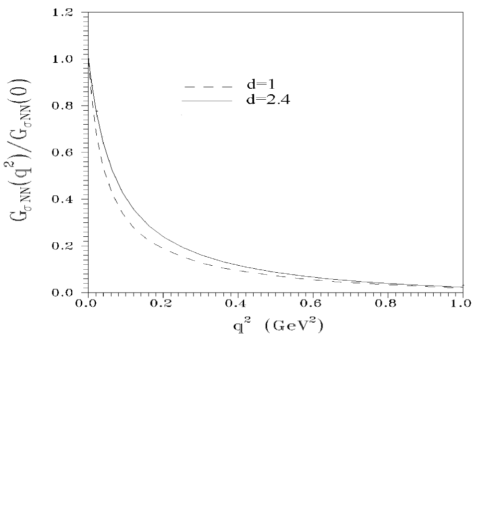
FIG. 1.: The normalized $\sigma NN$ form factor, $G_{\sigma NN}(t)$. The solid and dashed lines are for $d=2.4$ and $d=1$ cases respectively.

REFERENCES

• [1] Ulf-G. Meißner, A. Rakhimov and U. Yakhshiev Phys.Lett. B473, (2000), 200.
• [2] R.J. Furnstahl, Hua-Bin Tang, Brian D. Serot, Phys. Rev. C52, (1995), 1368.
• [3] C. K. Kim, A. Rakhimov and J. H. Yee, Phys. Rev. B71, 024518 (2005).
• [4] J. Schechter Phys.Rev.D21, (1980), 3393.
• [5] Ulf-G. Meißner, N. Kaiser and W. Weise, Nucl. Phys. A466, (1987), 685.
• [6] T.D. Cohen, Phys. Rev., D34, (1986), 2187.
• [7] N. Kaiser, U. Vogl, W. Weise and Ulf-G. Meißner, Nucl. Phys. A484, (1988), 593.
• [8] R. Machleidt, K. Holinde and C. Elster, Phys. Rep. 149, (1987), 1.
• [9] G. Holzwarth and R. Machleidt, Phys. Rev. C55, (1997), 1088.
Refer to caption