Coordinate Space HFB Calculations for the
Zirconium Isotope Chain up to the Two-Neutron Dripline

Abstract

We solve the Hartree-Fock-Bogoliubov (HFB) equations for deformed, axially symmetric even-even nuclei in coordinate space on a 2-D lattice utilizing the Basis-Spline expansion method. Results are presented for the neutron-rich zirconium isotopes up to the two-neutron dripline. In particular, we calculate binding energies, two-neutron separation energies, normal densities and pairing densities, mean square radii, quadrupole moments, and pairing gaps. Very large prolate quadrupole deformations ($\beta_{2}=0.42,0.43,0.47$) are found for the ^102,104,112Zr isotopes, in agreement with recent experimental data. We compare 2-D Basis-Spline lattice results with the results from a 2-D HFB code which uses a transformed harmonic oscillator basis.

I Introduction

In contrast to the well-understood behavior near the valley of stability, there are many open questions as we move towards the neutron dripline. In this exotic region of the nuclear chart, one expects to see several new phenomena NNigata : the neutron-matter distribution is very diffuse giving rise to the “neutron skins” and the “neutron halos”. One also expects new collective modes associated with the neutron skin, e.g. the “scissors” vibrational mode.

In current experiments, the neutron dripline has only been reached for relatively light nuclei. The second-generation radioactive ion beam (RIB) facilities currently under construction will allow us to explore nuclear structure and astrophysics at the driplines of heavier nuclei.

It is generally acknowledged that an accurate theoretical treatment of the pairing interaction is essential for a description of the exotic nuclei TOU03 ; OU03 . Besides large pairing correlations, the HFB calculations have to face the problem of an accurate description of the continuum states with a large spatial extent. All of these features represent major challenges for the numerical solution.

There are various mean-field methods of solving the non-relativistic HFB equations. Generally, they can be divided into two categories: lattice methods and basis expansion methods. In the lattice approach no region of the spatial lattice is favored over any other region: the well bound, weakly bound and (discretized) continuum states can be represented with the same accuracy. Currently, there are only two codes which solve the HFB problem on a lattice in coordinate space without any approximations using the quasiparticles: a 1-D (spherical) HFB code DN96 and the present 2-D (axially symmetric) code TOU03 ; OU03 ; OU04 . In the basis expansion method a wave function is expanded into the chosen basis functions: the harmonic oscillator basis (HO) egidorobledo , the transformed harmonic oscillator basis (THO) Stoitsov:2003pd , the HF orbitals yamagami ; Terasaki:1995du . There is also an alternative method that is under development where the HFB equations are solved in the 3-D Cartesian mesh using the canonical-basis approach Tajima2003 .

We solve the Hartree-Fock-Bogoliubov (HFB) equations for deformed, axially symmetric nuclei in coordinate space on a 2-D lattice TOU03 ; OU03 . Our computational technique (the Basis-Spline collocation and Galerkin method) is particularly well suited to study the ground state properties of nuclei near the driplines. It allows us to take into account high-energy continuum states up to an equivalent single-particle energy of 60 MeV or more.

In this paper we study the ground state properties of neutron-rich zirconium nuclei ($Z=40$) up to the two-neutron dripline. The isotope chain calculations start from the ¹⁰²Zr isotope up to the dripline nucleus, which turns out to be ¹²²Zr. For a long time, the $A\sim 100$ region has been of interest to nuclear structure physicists as an area of competition between various coexisting nuclear shapes (well-deformed prolate, oblate, or spherical) Ca02 . The zirconium isotopes are known to possess a rapidly changing nuclear shape when the neutron number changes from 56 to 60 R-A04 . We find that a spherical ground state shape is preferred over a prolate shape starting from the ¹¹⁴Zr isotope up to the dripline nucleus ¹²²Zr. In this paper, we compare Basis-Spline lattice results with the HFB-2D-THO code Stoitsov:2003pd , which uses a transformed harmonic oscillator basis (THO), as well as with currently available experimental data.

II Skyrme-HFB equations in coordinate space

A detailed description of the Basis-Spline lattice method has been published in references TOU03 ; OU03 ; we give here only a brief summary. In coordinate space representation, the HFB Hamiltonian and the quasiparticle wavefunctions depend on the distance vector ${\bf r}$, spin projection $\sigma=\pm\frac{1}{2}$, and isospin projection $q=\pm\frac{1}{2}$ (corresponding to protons and neutrons, respectively). In the HFB formalism, there are two types of quasiparticle (bi-spinor) wavefunctions, $\phi_{1}$ and $\phi_{2}$. In the present work, we utilize a Skyrme effective N-N interaction in the particle-hole channel while the $p-p$ and $h-h$ channels are described by a zero-range delta pairing force. For these types of effective interactions, the particle mean field Hamiltonian $h$ and the pairing field Hamiltonian $\tilde{h}$ are diagonal in isospin space and local in position space, and the HFB equations have the following structure TOU03 :

$$\left(\begin{array}[]{cc}(h^{q}-\lambda)&\tilde{h}^{q}\\ \tilde{h}^{q}&-(h^{q}-\lambda)\end{array}\right)\left(\begin{array}[]{c}\phi^{q}_{1,\alpha}\\ \phi^{q}_{2,\alpha}\end{array}\right)=E_{\alpha}\left(\begin{array}[]{c}\phi^{q}_{1,\alpha}\\ \phi^{q}_{2,\alpha}\end{array}\right),$$ (1)

where the Lagrange parameter $\lambda$ is introduced to yield the correct particle-number on average since the HFB wavefunction does not have a well defined particle-number.

The quasiparticle energy spectrum is discrete for $|E|<-\lambda$ and continuous for $|E|>-\lambda$ DN96 . For even-even nuclei it is customary to solve the HFB equations for positive quasiparticle energies and consider all negative energy states as occupied in the HFB ground state. The quasiparticle wavefunctions determine the normal density $\rho_{q}({\bf r})$ and the pairing density $\tilde{\rho}_{q}({\bf r})$ as follows

$$\rho_{q}({\bf r})\ = \ \sum_{E_{\alpha}>0}^{\infty}\sum_{\sigma=-\frac{1}{2}}^{+\frac{1}{2}}\phi^{q}_{2,\alpha}({\bf r}\sigma)\ \phi^{q\ *}_{2,\alpha}({\bf r}\sigma)\ ,$$ (2)

$$\tilde{\rho_{q}}({\bf r})\ = \ -\sum_{E_{\alpha}>0}^{\infty}\sum_{\sigma=-\frac{1}{2}}^{+\frac{1}{2}}\phi^{q}_{2,\alpha}({\bf r}\sigma)\ \phi^{q\ *}_{1,\alpha}({\bf r}\sigma)\ .$$ (3)

Restricting ourselves to axially symmetric nuclei, we use cylindrical coordinates $(r,z,\phi)$. In the HFB lattice method, we introduce a 2-D grid $(r_{\alpha},z_{\beta})$ with $\alpha=1,...,N_{r}$ and $\beta=1,...,N_{z}$. In radial direction, the grid spans the region from $0$ to $r_{max}$. Because we want to be able to treat octupole shapes, we do not assume left-right symmetry in $z$-direction. Consequently, the grid extends from $-z_{max}$ to $+z_{max}$. Typically, $z_{max}\approx r_{max}$ and $N_{z}$ $\approx$ $2\cdot N_{r}$. The HFB wavefunctions and operators are represented on the 2-D lattice by Basis-Spline expansion techniques. In practice, B-Splines of order M=9 are being used. Details about the B-Spline collocation and Galerkin methods are given in the Appendix.

III Numerical results and comparison with experimental data

This section describes the numerical results for the even-even members of the zirconium ($Z=40$) isotope chain up to the two-neutron dripline. Two theoretical approaches are presented and compared: a) a 2-D lattice method using B-Spline technology (hereafter referred to as HFB-2D-LATTICE), and b) an expansion in a 2-D harmonic oscillator (HFB-2D-HO) and transformed harmonic oscillator basis (HFB-2D-THO). We also compare theoretical results with experimental data whenever possible.

In all calculations we utilize the SLy4 Skyrme force CB98 and a zero-range pairing force with a strength parameter $V_{0}=-187.1305$ (HFB-2D-LATTICE code) and an equivalent single particle energy cutoff parameter of $\varepsilon_{max}=60$ MeV. The pairing strength V₀ has been adjusted in both codes to reproduce the measured average neutron paring gap of $1.245$ MeV in ¹²⁰Sn DN96 , as can be seen from Table 1.

Table 1: Results for ${}^{120}_{\ 50}Sn$. Comparison of results obtained from the HFB-2D-LATTICE code (first row) with HFB-2D-THO results (second row) and the experiment (third row). The columns display binding energies (BE), intrinsic quadrupole moments for neutrons and protons (Q_n,Q_p), rms-radii (r_n,r_p), average pairing gaps ($\Delta_{n},\Delta_{p}$), pairing energy for neutrons (PE_n), and Fermi levels ($\lambda_{n},\lambda_{p}$).

	BE(MeV)	Qn(fm2)	Qp(fm2)	rn(fm)	rp(fm)
	-1019.26	0.29	0.12	4.725	4.590
	-1018.22	0.00	0.00	4.728	4.593
	-1020.54	-	-	-	-
	$\Delta_{n}$(MeV)	$\Delta_{p}$(MeV)	PEn(MeV)	$\lambda_{n}$(MeV)	$\lambda_{p}$(MeV)
	1.244999	0.0	-10.24	-7.98	-8.16
	1.245469	0.0	-10.26	-7.99	-11.13
	1.245	-	-	-	-

In Table 1 we compare the results from the two HFB codes for the ${}^{120}_{\ 50}$Sn isotope. All observables agree very well. The apparent “disagreement” in the proton Fermi level $\lambda_{p}$ is really an artifact: the pairing gap vanishes at the magic proton number $Z=50$ resulting in an ill-defined Fermi energy. The two codes use different prescriptions for calculating $\lambda_{p}$ in the trivial case of no pairing. HFB+THO accepts the last occupied equivalent single-particle energy as $\lambda_{p}$ in this no pairing case, whereas the Basis-Spline code takes the average of the last occupied and first unoccupied equivalent single-particle energy levels.

III.1 Deformations, dripline and pairing properties

Recently, triple-gamma coincidence experiments have been carried out with Gammasphere at LBNL HR03 which have determined half-lives and quadrupole deformations of the neutron-rich ${}^{102,104}Zr$ isotopes. The isotopes from that region are produced in the process of fission of transuranic elements and have been studied via $\gamma$-ray spectroscopy techniques. These medium-mass nuclei are among the most neutron-rich isotopes ($N/Z\approx 1.6$) for which spectroscopic data are available. Very large prolate quadrupole deformations ($\beta_{2}=0.43,0.45$) are found for the ^102,104Zr isotopes. Furthermore, the laser spectroscopy measurements Ca02 for the zirconium isotopes have yielded precise rms-radii in this region. Recently, an experiment has been carried out to measure the mass of the ¹⁰⁴Zr isotope R-A04 . It is therefore of a great interest to compare these data with the predictions of the self-consistent HFB mean field theory.

In radial ($r$) direction, the lattice extends from $0-15$ fm, and in symmetry axis ($z$) direction from $-15,...,+15$ fm, with a lattice spacing of about $0.8$ fm in the central region. Angular momentum projections $\Omega=1/2,3/2,...,21/2$ were taken into account. Figure 1 shows the calculated two-neutron separation energies for the zirconium isotope chain. The two-neutron separation energy is defined as

$$S_{2n}(Z,N)\ =\ E_{bind}(Z,N)\ -\ E_{bind}(Z,N-2)\;.$$ (4)

Note that in using this equation, all binding energies must be entered with a positive sign. The position of the two-neutron dripline is defined by the condition $S_{2n}(Z,N)\ =0$, and nuclei with negative two-neutron separation energy are unstable against the emission of two neutrons. As one can see, both codes (HFB-2D-THO and HFB-2D-LATTICE) predict the dripline nucleus to be at mass number $A=122$. In addition, we observe a very good agreement between the two codes in the whole mass region of the isotope chain. We also give a comparison with the latest available experimental data up to the isotope ¹¹⁰Zr audi2003 .

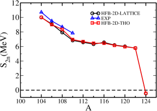
Figure 1: (Color online) Two-neutron separation energies for the neutron-rich zirconium isotopes. The dripline is located where the separation energy becomes zero. The ¹²²Zr isotope is the last stable nucleus against two neutron emission.

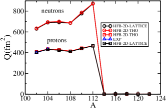
Figure 2: (Color online) Intrinsic quadrupole moments for protons and neutrons.

In Fig. 2 we compare the intrinsic proton and neutron quadrupole moments calculated with the lattice code and the THO code. Available experimental data HR03 are also given. Generally, we observe a nearly perfect agreement between the two codes as well as with the experiment. The deformations (for neutrons ) in terms of the deformation parameter $\beta_{2}$ for those nuclei, namely for the ^102-112Zr isotopes range from $\beta_{2}$=0.42 to $\beta_{2}=0.47$. Both the Basis-Spline lattice code and the HFB-2D-THO code predict the ¹¹²Zr isotope to have the largest ground state deformation. For mass numbers larger than 112, we observe spherical ground state shapes. Experimental deformations for protons are available for two isotopes, ¹⁰²Zr and ¹⁰⁴Zr HR03 . Calculations agree with the experiment reasonably well and give $\beta_{2}$ values of 0.42,0.43 while the experiment predicts $\beta_{2}^{102}$=0.42, $\beta_{2}^{104}$=0.45.

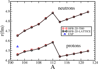
Figure 3: (Color online) Root-mean-square radii for the chain of zirconium isotopes.

In Fig. 3 we compare the root-mean-square radii of protons and neutrons predicted by the LATTICE code and the THO code. Both codes give nearly identical results for the whole isotope chain. Only one experimental data point is available, the proton rms radius of ¹⁰²Zr Ca02 . The experiment yields a proton rms radius of 4.54 fm while the HFB codes predict a value of 4.45 fm (HFB-2D-LATTICE) and 4.46 fm (HFB-2D-THO). The difference between theory and experiment is quite small, of order 2$\%$. We can clearly observe the presence of the neutron-skin manifested by the large differences between the neutron and proton rms radii for all of the isotopes in the chain. As expected the neutron-skin becomes ”thicker” as we approach the dripline. Starting at the mass number A=114 up to the dripline the nuclei prefer a spherical ground state shape (Fig. 2) which results in a sudden shrinking of the rms radius at A=114.

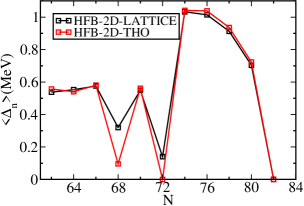
Figure 4: (Color online) Average neutron pairing gap for the chain of zirconium isotopes.

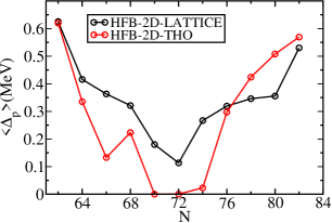
Figure 5: (Color online) Average proton pairing gap for the chain of zirconium isotopes.

Fig. 4 and Fig. 5 depict the average pairing gaps for neutrons and protons. Generally, both HFB codes show the same trend for the pairing gaps as a function of neutron number; the agreement is noticeably better for neutrons. The two HFB codes predict a small value of the neutron pairing gap for the ¹¹²Zr isotope which on the other hand has the largest prolate deformation (Fig. 2) among the calculated nuclei. Coincidentally, the dripline turns out to be at the neutron magic number (N=82) and, as expected, both codes yield a pairing gap of zero for the ¹²²Zr isotope.

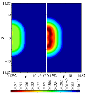
Figure 6: (Color online) Contour plots of the ¹¹⁰Zr normal densities, for protons (left) and neutrons (right). Densities are shown as a function of the cylindrical coordinates $(r,z)$, where $z$ is the symmetry axis.

III.2 Density studies

In this section we focus on the normal and pairing densities for the selected isotopes. In Fig. 6 we show a contour plot of normal densities for protons and neutrons for the ¹¹⁰Zr isotope. It is the last deformed isotope with a significant value of the pairing gap for neutrons, (Fig. 4), therefore it is possible to show plots of both normal and pairing densities. The results obtained for the neutron normal and pairing densities (Figs. 6 and 7) clearly exhibit a large prolate deformation. The normal density for neutrons (Fig. 6) is concentrated in the region that extends from $0$ fm to $2$ fm in $r$-direction and from $-5$ fm to $+5$ fm in $z$-direction. Within this region, we find an enhancement in the neutron density with a shape that resembles the figure “eight”. In comparing the neutron to the proton density, one notices that both the center of the nucleus and the surface is dominated by neutrons.

The pairing density for neutrons in Fig. 7 shows a richer structure than the normal density. This quantity describes the probability of correlated nucleon pair formation with opposite spin projection, and it determines the pair transfer formfactor. We can see that most correlated pair formation takes place in the four closed shaped structured areas near the z-axis. We may conclude that neutrons dominate the pairing properties in the interior of this nucleus. The same applies to normal densities (Fig. 6), yet the difference between neutrons and protons is more pronounced in case of the pairing densities. A graph depicting the single-particle energy spectrum of the pairing density for the ${}^{104}Zr$ isotope has been published in Ref. OU04 .

In Figs. 8 and 9 we show plots of normal densities as a function of the distance from the center, $r={\sqrt{\rho^{2}+z^{2}}}$. For a given value of $r$, the density is single-valued for a spherical nucleus and multi-valued for a deformed density distribution because in the latter case different combinations of lattice points $z_{i}$ and $\rho_{j}$ give rise to the same $r$-value.

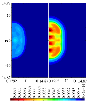
Figure 7: (Color online) Contour plots of the ¹¹⁰Zr pairing densities, for protons (left) and neutrons (right). The densities are shown as a function of the cylindrical coordinates $(r,z)$, where $z$ is the symmetry axis.

In Fig. 8 we compare three different calculations of the neutron normal density for the most deformed ¹¹²Zr isotope. The plot on a logarithmic scale shows that the density distribution predicted by the HFB-2D-THO and HFB-2D-LATTICE codes is deformed for almost all values of the distance from the nuclear center, $r$. At very large distances the densities become less deformed since nuclear potentials go to zero and HFB equations lead to a spherical asymptotic solution. Fig. 8 also shows for comparison the HFB-2D-HO result as an illustration of the shortcomings of the pure harmonic oscillator basis calculations to reproduce density distributions asymptoticly at very large distances. One can see its too rapid decay beyond distances of about 12 fm. Clearly, the pure harmonic oscillator basis calculations cannot represent properly density asymptotic for nuclei close to the neutron drip line.

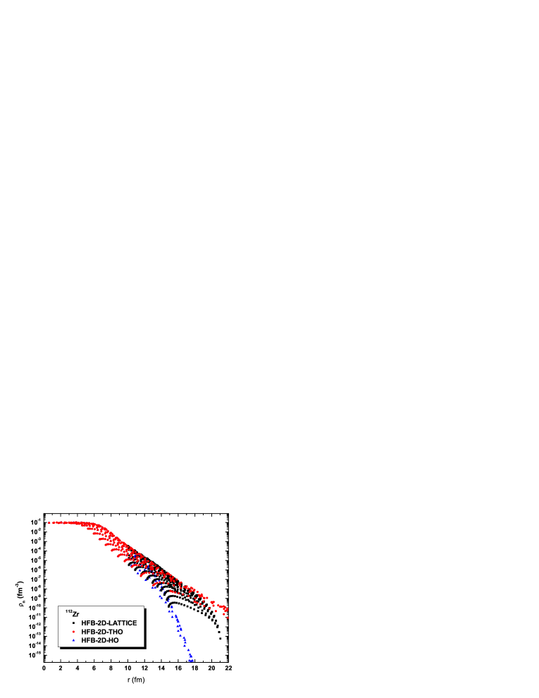
Figure 8: (Color online) Logarithmic plot of the normal neutron density for the most deformed isotope ¹¹²Zr as a function of the distance $r={\sqrt{\rho^{2}+z^{2}}}$.

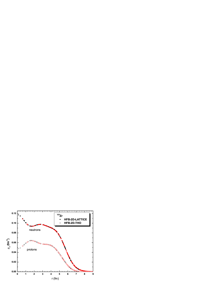
Figure 9: (Color online) Linear plot of the normal neutron and proton density for the dripline nucleus ¹²²Zr as a function of distance $r={\sqrt{\rho^{2}+z^{2}}}$. Comparison between the HFB-2D-THO code and the HFB-2D-LATTICE code.

Neutron and proton normal densities for the drip-line nucleus ¹²²Zr are shown in Fig. 9. From the single-valued plot as a function of $r={\sqrt{\rho^{2}+z^{2}}}$ one can immediately conclude that both neutron and proton normal densities are spherical. Another striking feature is a strong neutron enhancement at the center and a corresponding depletion in the proton density. Note also that the neutron density is substantially larger than the proton density for all values of $r$.

IV Conclusions

In this paper, we have performed Skyrme-HFB calculations in coordinate space for the neutron-rich zirconium isotopes up to the two-neutron dripline. We have calculated the ground state properties (even-even nuclei) for the zirconium isotopes (Z=40), starting from N=62 up to the two-neutron dripline, which our HFB codes predict to be N=82. In particular, we have calculated the two-neutron separation energies, quadrupole moments, rms radii, average pairing gaps and densities. In comparing HFB-2D-LATTICE theoretical calculations for the two-neutron separation energies (Fig. 1) with the HFB-2D-THO code we find the same results. Particularly, both codes predict the ¹²²Zr isotope to be the dripline nucleus. We find very large prolate deformations for the ^102-112Zr isotopes and a spherical ground state shape for the ^114-122Zr nuclei. The $\beta_{2}$ value for the most deformed nucleus ¹¹²Zr in the calculated chain reaches an impressive value of 0.47. The root-mean-square radii clearly show the existence of a “neutron skin” in the neutron-rich zirconium isotopes. We can also observe a sudden shrinking of the rms-radius at A=114 due to a change of the prolate ground state deformation into the spherical shape. In section III.B. we studied normal and pairing densities. In particular, Figures 6 and 7 show the dominant nature of neutrons, where one can observe that both normal and pairing densities are dominated by neutrons. The density studies in Figure 9 predict the presence of a sizable neutron skin in the spherical dripline nucleus ¹²²Zr.

*

Appendix A Basis-Spline representation of wavefunctions and operators

In this appendix, we discuss the representation of differential operators and wavefunctions in terms of Basis-Splines which is used in the HFB-2D-LATTICE code. There exists an extensive literature on Basis-Spline theory developed by mathematicians DeB78 . We have adapted some of these methods for the numerical solution of problems in atomic and nuclear physics on a lattice. Ref. Uma91 discusses the B-Spline collocation method, periodic and fixed boundary conditions, and the solution of various 1-D radial problems (Schrödinger, Poisson and Helmholtz equations) and the solution of 3-D Cartesian problems (Poisson equation). In a later paper, Umar et al. Uma91a solved the HF and TDHF equations on a 3-D lattice. In 1995, Wells et al. WO95 applied the B-Spline collocation method to the static and time-dependent Dirac equation which eliminated the “fermion doubling problem” that one encounters with the finite-difference method. In 1996, Kegley et al. KO96 studied 2-D axially symmetric systems in cylindrical coordinates with the collocation method and also introduced the Basis-Spline Galerkin method. In the following, we compare both of these methods.

A.1 HFB lattice representation

For the lattice representation of wavefunctions and operators, we use a Basis-Spline method. Basis-Spline functions $B_{i}^{M}(x)$ are piecewise-continuous polynomials of order $(M-1)$. They represent generalizations of finite elements which are B-splines with $M=2$.

We consider an arbitrary (differential) operator equation

$${\cal{O}}\bar{f}(x)-\bar{g}(x)=0\;.$$ (5)

Special cases include eigenvalue equations of the HF/HFB type where ${\cal{O}}=h$ and $\bar{g}(x)=E\bar{f}(x)$. We assume that both $\bar{f}(x)$ and $\bar{g}(x)$ are well approximated by spline functions

$$\bar{f}(x)\approx f(x) \equiv \sum_{i=1}^{\cal N}\mbox{$\displaystyle B^{M}_{i}$}(x)a^{i}\;,$$

$$\bar{g}(x)\approx g(x) \equiv \sum_{i=1}^{\cal N}\mbox{$\displaystyle B^{M}_{i}$}(x)b^{i}\;.$$ (6)

Because the functions $f(x)$ and $g(x)$ are approximations to the exact functions $\bar{f}(x)$ and $\bar{g}(x)$, the operator equation will in general only be approximately fulfilled

$${\cal{O}}f(x)-g(x)=R(x)\;.$$ (7)

The quantity $R(x)$ is called the residual; it is a measure of the accuracy of the lattice representation.

A.2 Basis-Spline collocation method

In the collocation method, one minimizes the residual locally, i.e. one introduces a set of collocation (data) points $x_{\alpha}$ and requires that the residual vanish exactly at these points

$$R(x_{\alpha})=0\ .$$ (8)

We multiply Eq.(7) from the left with $\delta(x-x_{\alpha})$ and integrate over x, including a volume element weight function $v(x)$ in the integrals to emphasize that the formalism applies to arbitrary curvilinear coordinates. Most cases of interest are covered by a function of the form

$$v(x)=x^{p}\;\;\;\;p=\left\{\begin{array}[]{ll}0&\mbox{Cartesian}\\ 1&\mbox{Polar}\\ 2&\mbox{Spherical}\end{array}\right.\;.$$ (9)

Using the collocation condition Eq.(8) one obtains

$$[{\cal{O}}f(x)]_{x_{\alpha}}-g(x_{\alpha})=0\ .$$ (10)

Inserting the B-Spline expansion (A.1) of the function $f(x)$ this results in

$$\sum_{i}[{\cal{O}}B]_{\alpha i}a^{i}-g(x_{\alpha})=0\ ,$$ (11)

where we have introduced the shorthand notation

$$[{\cal{O}}B]_{\alpha i}=[{\cal{O}}B_{i}(x)]_{x_{\alpha}}\;.$$ (12)

We eliminate the expansion coefficients $a^{i}$ in Eq.(11) by introducing the function values at the lattice support points $x_{\alpha}$ including both interior and boundary points

$$f_{\alpha}=f(x_{\alpha})=\sum_{i}B_{i}(x_{\alpha})a^{i}=\sum_{i}B_{\alpha i}a^{i}\;,$$ (13)

$$g_{\alpha}=g(x_{\alpha})=\sum_{i}B_{i}(x_{\alpha})b^{i}=\sum_{i}B_{\alpha i}b^{i}\;.$$ (14)

The matrix $B_{\alpha i}$ is, in general, rectangular. However, it can be made into a square matrix by adding either periodic or fixed boundary conditions; this is described in detail in references Uma91 ; WO95 ; KO96 . In what follows, the new (square) B-Spline matrix with the boundary conditions added is also denoted by $B_{\alpha i}$, for simplicity of notation. Because the matrix $B$ is now a square matrix it can be inverted to eliminate the expansion coefficients $a^{i},\ b^{i}$

$$a^{i}=\sum_{\alpha}B^{i\alpha}f_{\alpha}\;\;\;,\;\;\;b^{i}=\sum_{\alpha}B^{i\alpha}g_{\alpha}\;,$$ (15)

resulting in

$$\sum_{\beta}\sum_{i}[{\cal{O}}B]_{\alpha i}B^{i\beta}f_{\beta}=g_{\alpha}\;.$$ (16)

Defining the collocation lattice representation of the operator ${\cal{O}}$ via

$${\cal{O}}_{\alpha}^{\beta}=\sum_{i}[{\cal{O}}B]_{\alpha i}B^{i\beta}\;,$$ (17)

we arrive at the desired lattice representation

$$\sum_{\beta}{\cal{O}}_{\alpha}^{\beta}f_{\beta}=g_{\alpha}\ .$$ (18)

A.3 Basis-Spline Galerkin method

To derive the Galerkin representation, we multiply Eq.(7) from the left with the spline function $B_{k}(x)$ and integrate over $x$

$$\int v(x)dxB_{k}(x){\cal{O}}f(x)-\int v(x)dxB_{k}(x)g(x)=$$

$$\int v(x)dxB_{k}(x)R(x)\;.$$ (19)

Various schemes exist to minimize the residual function $R(x)$; in the Galerkin method one requires that there be no overlap between the residual and an arbitrary B-spline function

$$\int v(x)dxB_{k}(x)R(x)\stackrel{{\scriptstyle!}}{{=}}0\;.$$ (20)

This so called Galerkin condition amounts to a global reduction of the residual. We apply the Galerkin condition to Eq.(A.3) and insert the B-Spline expansions for $f(x)$ and $g(x)$, Eq.(A.1), resulting in

$$\sum_{i}\left[\int v(x)dxB_{k}(x){\cal{O}}B_{i}(x)\right]a^{i} -$$

$$\sum_{i}\left[\int v(x)dxB_{k}(x)B_{i}(x)\right]b^{i} = 0\;.$$ (21)

Defining the matrix elements

$${\cal{O}}_{ki} = \int v(x)dxB_{k}(x){\cal{O}}B_{i}(x)\;,$$ (22)

$$G_{ki} = \int v(x)dxB_{k}(x)B_{i}(x)\;\;.$$ (23)

transforms the (differential) operator equation into a matrix $\times$ vector equation

$$\sum_{i}{\cal{O}}_{ki}a^{i}=\sum_{i}G_{ki}b^{i}\;.$$ (24)

which can be implemented on modern vector or parallel computers with high efficiency. The matrix $G_{ki}$ is sometimes referred to as the Gram matrix; it represents the non vanishing overlap integrals between different B-Spline functions. This matrix possesses several highly desirable numerical properties; it is symmetric, banded, positive definite, and invertible for any reasonable placement of the knots and any spline order

$$\sum_{k}G^{jk}G_{ki}=\delta^{j}_{i}\;.$$ (25)

We use again the relations (15) to eliminate the expansion coefficients $a^{i}$ and $b^{i}$ in Eq.(24) which results in the matrix equation on the Galerkin lattice

$$\sum_{\beta}{\cal{O}}_{\alpha}^{\beta}f_{\beta}=g_{\alpha}\;,$$ (26)

with the differential operator definition on the Galerkin lattice

$${\cal{O}}_{\alpha}^{\beta}=\sum_{ijk}B_{\alpha i}G^{ij}{\cal{O}}_{jk}B^{k\beta}\;.$$ (27)

We are also extending our previous B-spline work to include nonlinear grids. Use of a nonlinear lattice should be most useful for loosely bound systems near the proton or neutron drip lines. Non-Cartesian coordinates necessitate the use of fixed endpoint boundary conditions; much effort has been directed toward improving the treatment of these boundaries.

A.4 2-D lattice representation of HFB wavefunctions and Hamiltonian

For a given angular momentum projection quantum number $\Omega$, we solve the eigenvalue problem on a 2-D grid $(r_{\alpha},z_{\beta})$ where $\alpha=1,...,m$ and $\beta=1,...,n$.

The four components of the spinor wavefunction $\psi^{(4)}(r,z)$ are represented on the 2-D lattice by a product of Basis Spline functions $B_{i}(x)$ evaluated at the lattice support points. For example, the spin-up component of the wavefunction $\phi_{2}$ is represented in the form

$$\phi_{2}^{\Omega}(r_{\alpha},z_{\beta},\uparrow)=\sum_{i,j}B_{i}^{M}(r_{\alpha})\ B_{j}^{M}(z_{\beta})\ U_{2}^{ij}\ .$$ (28)

Hence, the four-dimensional spinor wavefunction in coordinate space $\psi^{(4)}(r,z)$ becomes an array $\psi(N)$ of length $N=4\cdot m\cdot n$.

For the lattice representation of the HFB Hamiltonian, we use a hybrid method in which derivative operators are constructed using the Galerkin method; this amounts to a global error reduction. Local potentials are represented by the B-Spline collocation method (local error reduction).

The lattice representation transforms the differential operator equation into a matrix $\times$ vector equation

$$\sum_{\nu=1}^{N}{\cal{H}}_{\mu}^{\ \nu}\psi^{\Omega}_{\nu}=E^{\Omega}_{\mu}\psi^{\Omega}_{\mu}\ \ \ (\mu=1,...,N)\ .$$ (29)

The 2-D HFB code is written in Fortran 95 and makes extensive use of new data concepts, dynamic memory allocation and pointer variables.

A.5 2-D B-Spline Poisson Solver

In the current version of our HFB-2D-LATTICE code we have solved the Poisson equation in cylindrical coordinates $(\rho,z)$

$$\frac{\partial^{2}\phi(\rho,z)}{\partial\rho^{2}}+\frac{\phi(\rho,z)}{4\rho^{2}}+\frac{\partial^{2}\phi(\rho,z)}{\partial z^{2}}=-4\pi e^{2}\sqrt{\rho}\ \rho_{p}(\rho,z)\;,$$

by applying a large distance expansion of the Coulomb potential $(|{\bf r}|\gg|{\bf r}^{\prime}|)$

$$\phi_{c}({\bf r})=e\int{\frac{\rho_{p}({\bf r}^{\prime})}{|{\bf r}-{\bf r}^{\prime}|}d^{3}{\bf r}^{\prime}},$$ (30)

$$\frac{1}{|{\bf r}-{\bf r}^{\prime}|} = e^{-{\bf r}^{\prime}\cdot\vec{\bigtriangledown}}\frac{1}{|{\bf r}|}=\frac{1}{r}-{\bf r}^{\prime}\cdot\vec{\bigtriangledown}\frac{1}{r}+\frac{1}{2}\left({\bf r}^{\prime}\cdot\vec{\bigtriangledown}\right)^{2}\frac{1}{r}$$

$$- \frac{1}{6}\left({\bf r}^{\prime}\cdot\vec{\bigtriangledown}\right)^{3}\frac{1}{r}+\frac{1}{24}\left({\bf r}^{\prime}\cdot\vec{\bigtriangledown}\right)^{4}\frac{1}{r}+\ldots,$$

with the following boundary conditions

$$\phi_{c}(\rho\rightarrow 0,z) \rightarrow 0\;,$$

$$\phi_{c}(\rho,z\rightarrow z_{max}) \rightarrow 0\;.$$ (31)

The differential operators are represented on the lattice using the B-Spline Galerkin method.

- (1) J. Dobaczewski, N. Michel, W. Nazarewicz, M. Ploszajczak, and M.V. Stoitsov, in “A New Era of Nuclear Structure Physics”, ed. Y. Suzuki, S. Ohya, M. Matsuo & T. Ohtsubo, World Scientific (2004), pp.162-171.
- (2) E. Terán, V.E. Oberacker, and A.S. Umar, Phys. Rev. C 67, 064314 (2003).
- (3) V.E. Oberacker, A.S. Umar, E. Terán, and A. Blazkiewicz, Phys. Rev. C 68, 064302 (2003).
- (4) J. Dobaczewski, W. Nazarewicz, T.R. Werner, J.F. Berger, C.R. Chinn, and J. Dechargé, Phys. Rev. C 53, 2809 (1996).
- (5) V.E. Oberacker, A.S. Umar, A. Blazkiewicz, and E. Terán, in “A New Era of Nuclear Structure Physics”, ed. Y. Suzuki, S. Ohya, M. Matsuo & T. Ohtsubo, World Scientific (2004), pp.179-183.
- (6) J.L. Egido, L. M. Robledo, and Y. Sun, Nucl. Phys. A560, 253 (1993).
- (7) M. V. Stoitsov, J. Dobaczewski, W. Nazarewicz, S. Pittel, and D. J. Dean, Phys. Rev. C 68, 054312 (2003).
- (8) M. Yamagami, K. Matsuyanagi, and M. Matsuo, Nucl. Phys. A693, 579 (2001).
- (9) J. Terasaki, P. H. Heenen, H. Flocard, and P. Bonche, Nucl. Phys. A 600, 371 (1996).
- (10) N. Tajima, Phys. Rev. C 69, 034305 (2004).
- (11) P. Campbell et al., Phys. Rev. Lett. 89, 082501 (2002).
- (12) S. Rinta-Antila, S. Kopecky, V.S. Kolhinen, J. Hakala, J. Huikari, A. Jokinen, A. Nieminen, and J. Äystö, Phys. Rev. C 70, 011301(R), (2004).
- (13) E. Chabanat, P. Bonche, P. Haensel, J. Meyer, and R. Schaeffer, Nucl. Phys. A635, 231 (1998); Nucl. Phys. A643, 441 (1998).
- (14) Half lives of isomeric states from SF of 252Cf and large deformations in 104Zr and 158Sm, J.K. Hwang, A.V. Ramayya, J.H. Hamilton, D. Fong, C.J. Beyer, P.M. Gore, E.F. Jones, E. Terán, V.E. Oberacker, A.S. Umar, Y.X. Luo, J.O. Rasmussen, S.J. Zhu, S.C. Wu, I.Y. Lee, P. Fallon, M.A. Stoyer, S. J. Asztalos, T.N. Ginter, J.D. Cole, G.M. Ter-Akopian, and R. Donangelo, (in preparation).
- (15) P.-G. Reinhard, D.J. Dean, W. Nazarewicz, J. Dobaczewski, J. A. Maruhn, and M.R. Strayer, Phys. Rev. C 60, 014316 (1999).
- (16) M.V. Stoitsov, J. Dobaczewski, P. Ring, and S. Pittel, Phys. Rev. C 61, 034311 (2000).
- (17) M. Samyn, S. Goriely, M. Bender, and J. M. Pearson, Phys. Rev. C 70, 044309 (2004).
- (18) P. Ring, Prog. Part. Nucl. Phys. 37, 193 (1996).
- (19) G.A. Lalazissis, S. Raman, and P. Ring, Atomic Data and Nuclear Data Tables 71, 1 (1999).
- (20) G. Audi and A.H. Wapstra, Nucl. Phys. A595, 409 (1995); and “Table of Nuclides”, Brookhaven Nat. Lab.,http://www2.bnl.gov/ton/index.html.
- (21) G. Audi, A. H. Wapstra and C. Thibault, Nucl. Phys. A 729, 337-676 (2003).
- (22) C. De Boor, Practical Guide to Splines, (Springer Verlag, New York, 1978), and references therein.
- (23) A.S. Umar, J. Wu, M.R. Strayer, and C. Bottcher, J. Comp. Phys. 93, 426, (1991).
- (24) A.S. Umar, M.R. Strayer, J.-S. Wu, D.J. Dean, and M.C. Güçlü, Phys. Rev. C 44, 2512 (1991).
- (25) J.C. Wells, V.E. Oberacker, M.R. Strayer and A.S. Umar, Int. J. Mod. Phys. C 6, 143, (1995).
- (26) D.R. Kegley, V.E. Oberacker, M.R. Strayer, A.S. Umar, and J.C. Wells, J. Comp. Phys. 128, 197, (1996).