Properties of quark matter produced in heavy ion collision

Abstract

We describe the hadronization of quark matter assuming that quarks creating hadrons coalesce from a continuous mass distribution. The pion and antiproton spectrum as well as the momentum dependence of the antiproton to pion ratio are calculated. This model reproduces fairly well the experimental data at RHIC energies.

1 Introduction

The most important aim of heavy ion experiments performed at the RHIC accelerator besides the production of quark matter is the reconstruction of its properties from the observed hadron measurables.

The investigations of this problem are focused around three main questions: a) the effective mass of the quarks, b) the momentum distribution of quarks, c) the hadronization mechanism.

Regarding the quark mass in quark matter up to now essentially two different assumptions has been made: i) the quark matter consists of an ideal gas of non-interacting massless quarks and gluons and this type of quark matter undergoes a first order phase transition during the hadronization; or ii) the effective degrees of freedom in quark matter are dressed quarks with an effective mass of about $0.3$ GeV, which mass is the result of the interactions within the quark matter; this type of quark matter clusterizes and forms hadrons smoothly, following a cross-over type deconfinement – confinement transition.

Considering the momentum distribution in quark matter one meets the following ideas: The bulk part of the quarks is produced in soft processes, these quarks have a fairly exponential transverse momentum distribution on the top of a collective transverse flow in heavy ion collisions. On the other hand, quarks with large transverse momentum ($p_{T}\geq 2-4$ GeV) are viewed as produced mainly in hard collisions and their spectra obey a power law shape described by the functional form of fragmentation functions.

Finally one meets the worthy problem of hadronization. In early publications [1, 2] the hadronization was assumed to happen through a quasi-static, first order phase transition. However, as the experiments have suggested that the whole lifetime of the heavy ion collision is very short, other non-equilibrium dynamical models obtained more and more credit. One of the most successful description is based on quark coalescence [3, 4, 5, 6, 7, 8]. This idea is supported by recent RHIC experiments [9].

In this paper we present a new model of the late phase of the heavy ion collision. In this approach the effective quarks are massive and have a particular mass distribution described in Section 2. In Section 3 the quark momentum distribution is studied in details. Section 4 summarizes the appropriate expressions for the coalescence processes in this environment. Numerical results and comparison to experimental data are displayed in Section 5. We discuss the obtained results in Section 6.

2 Mass distribution of Quarks

We assume that in hot and dense deconfined matter the average interaction of the massless (current) quarks generate an effective mass for them. Several analyses of lattice QCD calculations supports the appearance of massive quark degrees of freedom [10, 11]. (According to these analyses the gluons become very heavy just before hadronization, and thus we neglect their explicit degrees of freedom in the models.) The mass of these quasi-particles is in the range of $0.3-0.4$ GeV around the phase transition temperature. In the early approaches the quasi-quarks have a sharp, momentum independent mass. In a realistic approach, however, there is no reason to assume that the interacting quarks behave as on-shell particles. Due to the residual interaction the mass of the quasi-quarks may be distributed in an interval of about a few hundred MeV while having a maximum in the range of $0.3-0.4$ GeV. The shape of this distribution is presently not known . One may want to investigate the effect of different spectral functions on the hadronization process. In the present work we consider the following mass distribution:

$$\rho(m)={\it N}e^{-\frac{\mu}{T_{c}}\sqrt{\frac{\mu}{m}+\frac{m}{\mu}}}$$ (1)

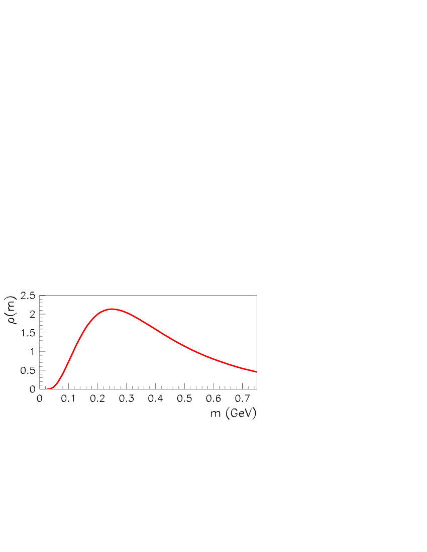
Figure 1: Distribution of the effective quark mass in eq. (1).

This distribution vanishes both for too small and too large masses and has a smooth maximum around the familiar valence quark mass value ($\mu$). Fig.1 displays this mass distribution for $\mu=0.25$ GeV and $T_{c}=0.26$ GeV.

3 Momentum distribution of quarks

In the RHIC experiments it was observed, that the produced particles show a nearly exponential spectrum at low transverse momenta and a power-law like one at high transverse momenta. This distribution was considered in earlier publications as a sum of three components produced by different physical mechanisms: a) thermal equilibrium, b) coalescence, c) fragmentation. The relative weights of these components were determined by a fit to the experimental data. In the present work we assume an analytic, parameterized transverse momentum distribution, which is similar to an exponential distribution for low momenta and a power law distribution for large momenta. The phase space density of effective quarks with a variable mass $m$, transverse momentum $p_{T}$, coming from an angular direction $\phi$ and a coordinate rapidity $\eta$ is given by

$$f_{quark}(p_{\perp},m,\phi,\eta)=\frac{A}{[1+(q-1)*\frac{E(p_{\perp},m,\phi,\eta)}{T}]^{(q/(q-1))}},$$ (2)

Here $q$ is a parameter characterizing a possible deviation from the usual Boltzmann distribution, which is recovered for $q=1$. The parameter $T$ is in general not the usual temperature, but in the Boltzmann limit, $q\rightarrow 1$ it becomes the canonical temperature. That which values of $q$ and $T$ fit experimental heavy ion data best, may depend on the transverse momentum range considered: a $q$ value not equal one fits usually to much higher momenta than the original Boltzmannian assumption.

Although the expression in eq. (2) coincides with the form of the Tsallis distribution [12] (as many simple minded fits do), we do not necessarily have to assume a special equilibrium state, which is considered in the non-extensive thermodynamics. One may assume such an equilibrium Tsallis system in quark matter if one of the following conditions is fulfilled: i) there is an energy dependent random noise in the system not reflecting a constant temperature; ii) the system contains a finite number of particles which interact indefinitely long; iii) there are long range forces in the system. We realize, that such conditions may be found in a fireball produced in high energy heavy ion collisions, it is just not sure, whether the time is enough to arrive at such a special equilibrium state.

The energy $E$, appearing in eq.(2) is given by the blast wave formula:

$$E(p_{\perp},m,\phi,\eta)=\gamma(\sqrt{m^{2}+p_{\perp}^{2}}\cdot\cosh(\eta)-v_{flow}\cdot p_{\perp}\cdot\cos(\phi)).$$ (3)

assuming a homogeneous transverse flow velocity, $v_{flow}$, with a corresponding Lorentz factor, $\gamma$. In eq.(3) the effect of an average ”blue shift”, caused by the hydrodynamical flow, is taken into account.

4 Coalescence of Massive Quarks

Using the covariant coalescence model of Dover et al. [13], the spectra of hadrons formed from the coalescence of quark and antiquarks can be written as

$$E\cdot\frac{dN_{h}}{d^{3}p}=\frac{dN_{h}}{dyp_{T}dp_{T}d\phi_{p}}=\frac{g_{h}}{(2\pi)^{3}}\int(p_{h}^{\mu}\cdot d\sigma_{h,\mu})F_{h}(x_{h};p_{h}).$$ (4)

Here $F_{h}(x_{h};p_{h})$ is an in principle eight dimensional distribution (Wigner function) of the formed hadron. Furthermore $d\sigma$ denotes an infinitesimal element of the space-like hypersurface where the hadrons are formed, while $g_{h}$ is the combinatorial factor for forming a colorless hadron from a spin 1/2 color triplet quark and antiquark. For pions the statistical is $g_{\pi}=1/36$ , for antiprotons $g_{\overline{p}}=1/108$ [6].

Assuming an instant hadronization at a sharp proper time, $\tau$, with cylindrical symmetry one gets

$$\frac{dN_{h}}{dyp_{T}dp_{T}d\phi_{p}}=\frac{g_{h}}{(2\pi)^{3}} \int \tau\cdot m_{\perp}cosh(y-\eta)d\eta rdrd\phi F_{h}(x_{h};p_{h})$$

Here $y$ is the momentum rapidity of the hadronic four-momentum $p_{h}$ and $\eta$ is the coordinate-rapidity of the formation point. For $y=0$ and $\phi=0$ eq.(4)becomes

$$\left.\frac{dN_{h}}{dyp_{T}dp_{T}d\phi_{p}}\right|_{y=0}=\frac{g_{h}}{(2\pi)^{3}}\cdot\pi R^{2}\tau\cdot m_{\perp}\cdot\int_{\Delta_{\eta}/2}^{\Delta_{\eta}/2}\!\!d\eta\>\cosh(\eta)\>F_{h}(p_{h};\eta)$$ (5)

Assuming that we get contribution to the spectra mainly from the $\Delta_{\eta}<<1$ region, eq.(5) simplifies to

$$\left.\frac{dN_{h}}{dyp_{T}dp_{T}d\phi_{p}}\right|_{y=0}\>=\>\frac{g_{h}}{(2\pi)^{3}}\cdot\pi R^{2}\tau\Delta_{\eta}\cdot m_{\perp}\cdot F_{h}(p_{h};0)$$ (6)

where $m_{\perp}=\sqrt{m^{2}+p_{T}^{2}}$ is the transverse mass, $\phi_{p}$ the angle of the transverse momentum of the hadron and $R$ is the cylindrical radius. Introducing the hadronization volume, $V=\Delta_{\eta}\tau R^{2}\pi$, and the abbreviation $F_{h}(p_{\perp},0)=F_{h}(p_{\perp})$ we finally get

$$\left.\frac{dN_{h}}{dyp_{T}dp_{T}d\phi_{p}}\right|_{y=0}\>=\>\frac{g_{h}}{(2\pi)^{3}}Vm_{\perp}F_{h}(p_{\perp})$$ (7)

Assuming that the mesons are produced by coalescence of particle a with mass $m_{a}$ and particle b with mass $m_{b}$ , the meson source function, $F_{M}({\bf p}_{M})$, will have the form:

$$F_{M}({\bf p}_{h})=\int d^{3}{\bf p}_{a}d^{3}{\bf p}_{b}f_{a}({\bf p}_{a};0)f_{b}({\bf p}_{b};0)C_{M}(p_{a},p_{b},p_{M}).$$ (8)

In eq.(8) the coalescence function $C_{M}(p_{a},p_{b},p_{M})$ is the probability for particles with four momenta $p_{a},p_{b}$ to form a meson with four momentum $p_{M}$. We assume a Gaussian wave-packet shape being maximal at zero relative momentum (characteristic for s-wave internal hadronic wave functions):

$$C_{M}(p_{a},p_{b},p_{M})=\alpha_{M}\cdot e^{-((p_{a}-p_{b})/P_{c})^{2}}$$ (9)

The parameters $\alpha_{M}$ and $P_{c}$ reflect properties of the hadronic wave function in the momentum representation convoluted with the formation matrix element. For the present consideration we assume that the system consist of a mixture of effective particles having different masses. The densities of particles with mass m are weighted with the corresponding mass distribution function, $\rho(m)$, eq.(1).

First we deal with the formation of mesons. We assume that the total mass and momentum of a hadron will be combined additively from that of the constituents, but $P_{c}$ is so small, that that practically zero relative momentum partons form a meson. This leaves us with

$${\bf p_{a}}={\bf p_{b}} = {\bf p_{M}}/2$$ (10)

$$m_{a}+m_{b} = m_{M}$$ (11)

This leads to the coalescence function

$$C_{M}=\alpha_{M}\cdot\delta(\vec{p}_{a}-\vec{p}_{M}/2)\cdot\delta(\vec{p}_{b}-\vec{p}_{M}/2)\cdot\delta(m_{a}+m_{b}-m_{M})$$ (12)

. Thus we arrive at the following meson distribution function:

$$F_{M}({\bf p_{t}};0)=\alpha_{M} \cdot \int_{0}^{m_{M}}dm_{a}\int_{0}^{m_{M}}dm_{b}\cdot\delta(m_{M}-(m_{a}+m_{b}))$$ (13)

$$\cdot \rho(m_{a})\cdot f_{q}({\bf p_{t}}/2;m_{a})$$

$$\cdot \rho(m_{b})\cdot f_{b}({\bf p_{t}}/2;m_{b}).$$

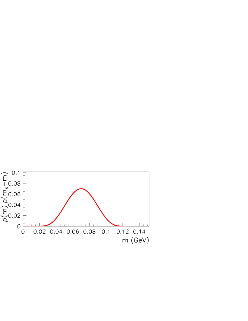
Figure 2: The product of the two quark-mass distributions, $\rho(m)\cdot\rho(m_{\pi}-m)$, in eq(13). The maximum of the product is at $m=m_{\pi}/2$.

Fig.2. shows the convolution of two quark-mass distribution functions appearing in the coalescence probability eq(13) for the coalescence production of a pion.

One observes, that the product of the two mass distributions always has a maximum around $m=m_{\pi}/2$. Already the naive coalescence approach works, whenever this maximum is sharp enough.

Similar argumentation leads to the three-fold coalescence expression. In the place of eq.(11) we get:

$${\bf p_{1}}={\bf p_{2}}={\bf p_{3}} = {\bf p_{B}}/3$$ (14)

$$m_{1}+m_{2}+m_{3} = m_{B}$$ (15)

and the baryon source function becomes

$$F_{B}(p_{t}) = \alpha_{B}\cdot\int_{0}^{m_{pr}}\!\!\!dm_{1}\int_{0}^{m_{pr}}\!\!\!dm_{2}\int_{0}^{m_{pr}}\!\!\!dm_{3}$$ (16)

. $$\rho(m_{1})\,f_{q}(p_{t}/3,m_{1}))$$

. $$\rho(m_{2})\,f_{q}(p_{t}/3,m_{2}))$$

. $$\rho(m_{3})\,f_{q}(p_{t}/3,m_{3}))\,\delta(m_{B}-(m_{1}+m_{2}+m_{3})).$$

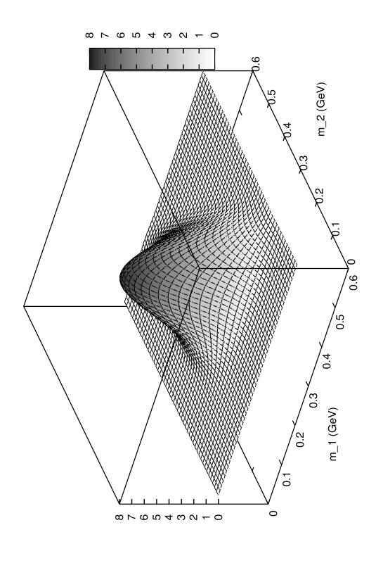
Figure 3: Product of three quark-mass distributions, $\rho(m_{1})\cdot\rho(m_{2})\cdot\rho(m_{3})$, from eq. (16). Horizontal axes connect to masses $m_{1}$ and $m_{2}$. Mass $m_{3}$ is defined as $m_{3}=m_{\overline{p}}-(m_{1}+m_{2})$.

Fig.3. shows the product of the three quark-mass distribution functions appearing in eq.(16).

Figures 2 and 3 shows that the maximum contribution to the coalescence integrals are obtained from the equal mass part of the mass distributions.

At the end of this section we may compare the basic philosophy of the different coalescence models. In all cases we met the problem of mismatch of initial and final state quantum numbers. To resolve this problem different solutions are proposed:

a) In the quantum mechanical approach the overlap of initial and final state wave function is calculated. In this process - simply said - the quantum mechanical uncertainty bridges the mismatch gap.

b) In the most often used classical approximation the coalescence probability is smeared around the momentum conservation, Ref. [13].

c) In the present approximation in the coalescence transition the momentum is strictly conserved, as in Ref. [7], but the masses of the particles of the initial state have a finite width distribution.

5 Numerical results and comparison with experimental data

The parameters used in the calculations are as follows. $\mu=0.25$ GeV, $T_{c}=0.26$ GeV, $T=0.07$ GeV, $q=1.19$, $v_{flow}=0.56$. The $\alpha_{M}$ and $\alpha_{B}$ coalescence constants were adjusted to fit the absolute value of the measured $\pi$ and $\overline{p}$ yields. In Fig.(4) both the $\pi^{-}$ and $\pi^{0}$ data are displayed.

In the Figures 4-6 we show the calculated distributions together with the corresponding experimental data. The experimental points are taken from Ref. [14].

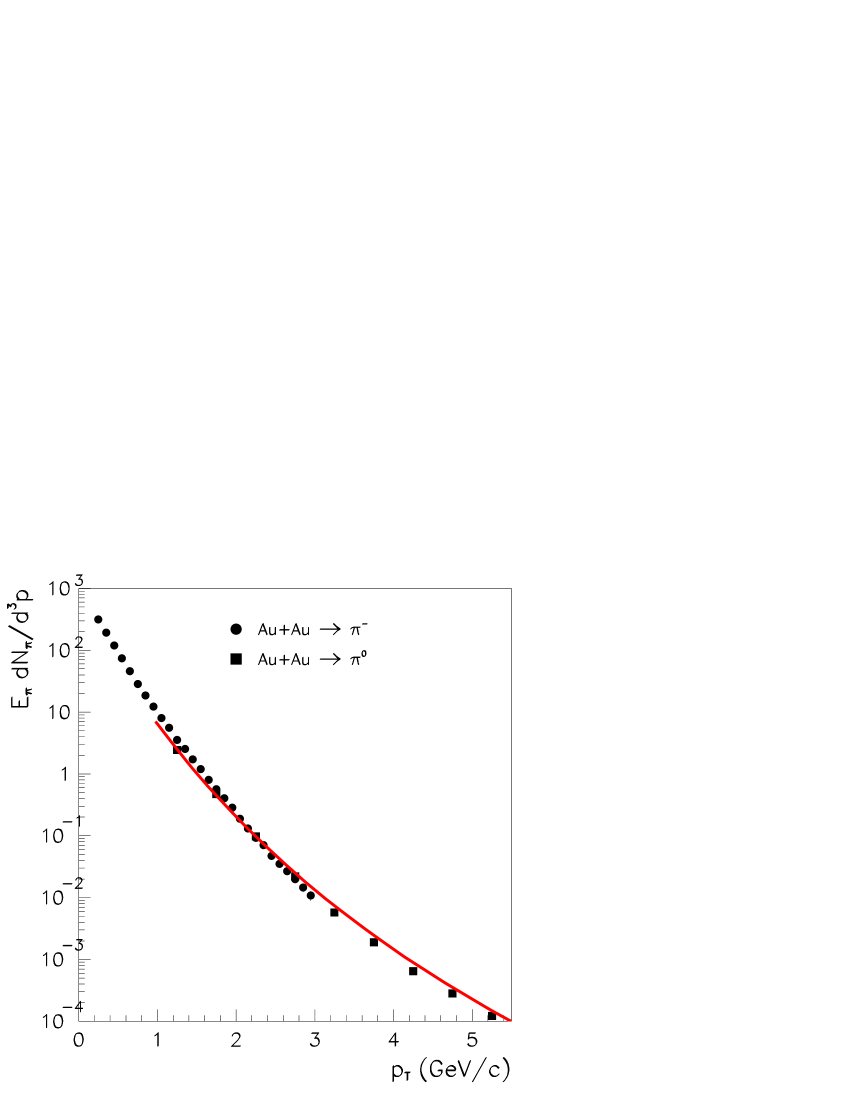
Figure 4: Measured pion spectra in central Au+Au collisions at $\sqrt{s}=200$ AGeV [14]. Full line indicates the calculated pion yield.

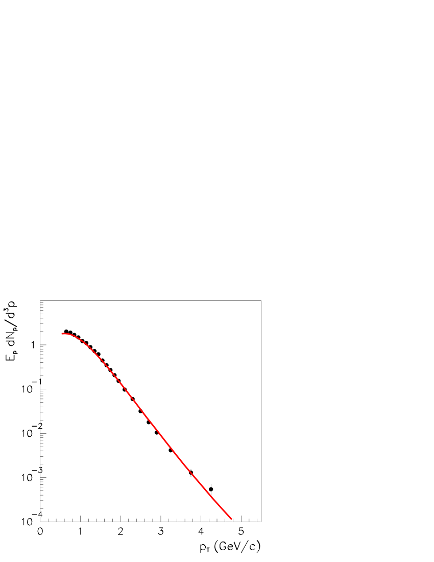
Figure 5: Transverse momentum spectrum for antiproton production in central Au+Au collisions at $\sqrt{s}=200$ AGeV [14]. Full line indicates our calculation.

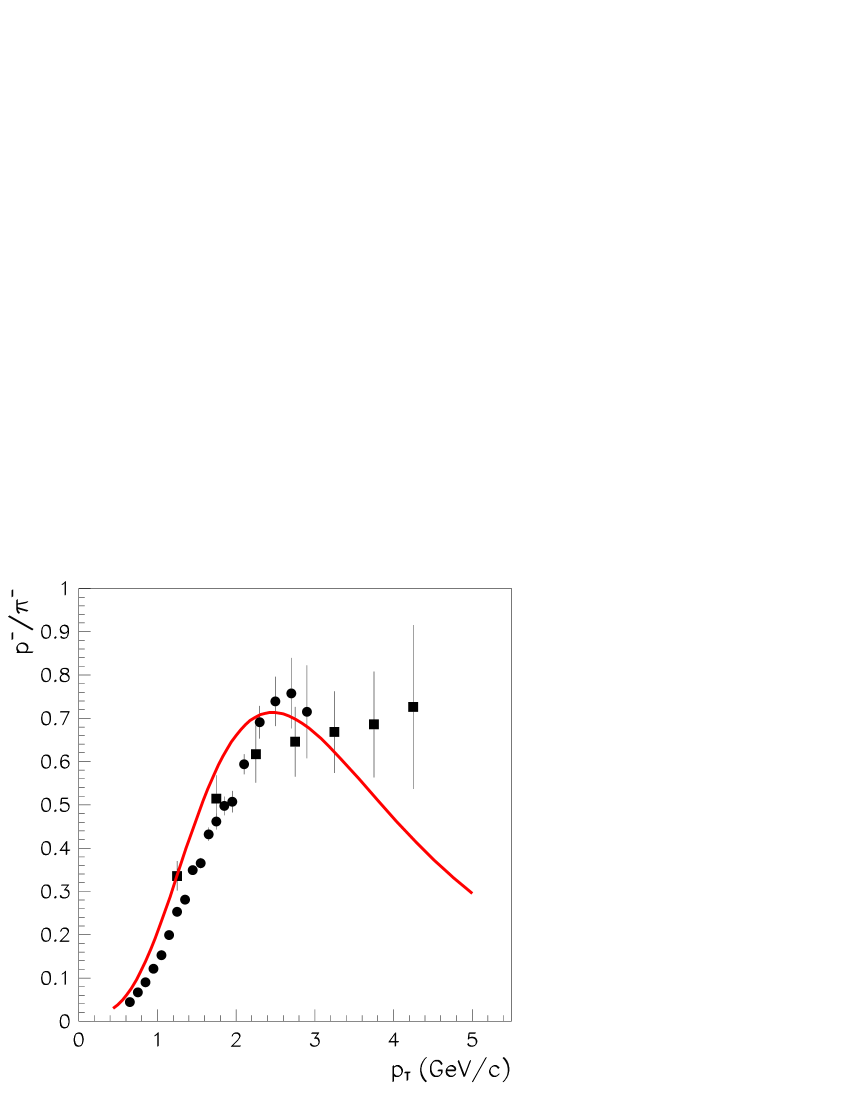
Figure 6: The ${\overline{p}}/\pi^{-}$ ratio as a function of $p_{T}$ on a linear scale in central Au+Au collisions at $\sqrt{s}=200$ AGeV [14].

6 Conclusion

In earlier publications [6, 7] it was assumed that for the low, medium and high transverse momentum intervals the hadrons are produced with different mechanisms, via thermal, coalescence and fragmentation processes. In the present work we proposed a model, in which, besides the momentum, the energy is also conserved to a good approximation in the coalescence process. This model yields results, which agree fairly well with experimental heavy ion data in the transverse momentum range from about 1 GeV to 8 GeV, (see Figs.(4) - (6)). This agreement supports the basic assumptions of our model: a) the masses of the partons have a finite width distribution (Fig.1); b) the momentum distribution of partons is described by one and the same function for a wide range of transverse momenta; c) the hadronization happens via effective quark coalescence; d) in the hadronization process both momentum and energy are nearly conserved locally.

Finally we note that a spherical inhomogeneity in the momentum distribution of the quarks leads to an azimuthal correlation of hadrons, if they are produced by the coalescence mechanism described in the present paper. This effect may be worth of a closer look in future studies.

References

References

- [1] Müller B (1985) The Physics of quark - gluon plasma, Lecture Notes in Physics vol.225, and references therein.
- [2] Biró T S and Zimányi J 1983 Nucl. Phys. A 395 525
- [3] Biró T S, Lévai P, and Zimányi J 1995 Phys. Lett. B347 6
- [4] Biró T S, Lévai P, and Zimányi J, 2001 J. Phys. G27 439; 2002 J. Phys. G28 1561
- [5] Hwa R C and Yang C B 2002 Phys. Rev. C66 025205; 2003 Phys. Rev. Lett. 90 212301; 2004 Phys. Rev. C70 024905
- [6] Greco V, Ko C M, and Lévai P 2003 Phys. Rev. Lett. 90 202302; Phys. Rev. C68 034904
- [7] Fries R J, Müller B, Nonaka C, and Bass S A 2003 Phys. Rev. Lett. 90 202303; Phys. Rev. C68 044902
- [8] Molnár D and Voloshin S A 2003 Phys. Rev. Lett. 91 092301; Lin Z and Molnár D 2003 Phys. Rev. C68 044901
- [9] Adams J et al. (STAR Collaboration) 2003 Phys. Lett. B567 167
- [10] Lévai P and Heinz U 1998 Phys. Rev. C57 1879
- [11] Peshier A, Kämpfer B, and Soff G 2000 Phys. Rev. C61 045203
- [12] Tsallis C 1988 J. Stat. Phys. 52 50; 1995 Physica A221 277; 1999 Preprint cond-mat/9903356
- [13] Dover C, Heinz U, Schnedermann E, and Zimányi J 1991 Phys. Rev. C44 1636
- [14] Adler S S, et al. (PHENIX Collaboration) 2004 Phys.Rev. C69 034909.