Sum Rule Approach to the Isoscalar Giant Monopole
Resonance in Drip Line Nuclei

Abstract

Using the density-dependent Hartree-Fock approximation and Skyrme forces together with the scaling method and constrained Hartree-Fock calculations, we obtain the average energies of the isoscalar giant monopole resonance. The calculations are done along several isotopic chains from the proton to the neutron drip lines. It is found that while approaching the neutron drip line, the scaled and the constrained energies decrease and the resonance width increases. Similar but smaller effects arise near the proton drip line, although only for the lighter isotopic chains. A qualitatively good agreement is found between our sum rule description and the presently existing random phase approximation results. The ability of the semiclassical approximations of the Thomas-Fermi type, which properly describe the average energy of the isoscalar giant monopole resonance for stable nuclei, to predict average properties for nuclei near the drip lines is also analyzed. We show that when $\hbar$-corrections are included, the semiclassical estimates reproduce, on average, the quantal excitation energies of the giant monopole resonance for nuclei with extreme isospin values.

I Introduction

Experimental and theoretical studies of exotic nuclei with extreme isospin values are presently one of the more active areas of research in nuclear physics. Recent developments in accelerator technology and detection techniques allow research beyond the limits of $\beta$-stability. The number of unstable nuclei for which masses have been measured is rapidly increasing R1 and this trend is expected to be continued due to the use of radioactive beams R1a ; R1b ; R1c . In particular, the proton drip line has been approached as far as for Pb isotopes R1d . The neutron drip line has been reached to date for $Z\leq 8$ and is expected to be extended to $Z\leq 28$ in the present decade R1e .

Collective phenomena are very useful tools to study the nuclear structure as well as to test the ability of the nuclear effective forces in describing such situations. The analysis of the small amplitude oscillations, i.e. the giant resonances, is of special relevance. In particular, it is very interesting to study the isoscalar giant monopole resonance (ISGMR) from where the incompressibility modulus of nuclear matter ($K_{\infty}$) can be extracted R14 ; R2 . The value of $K_{\infty}$ is an important ingredient not only for the description of finite nuclei but also for the study of heavy ion collisions, supernovae, and neutron stars.

The ISGMR for stable nuclei has been studied long ago from both, experimental and theoretical standpoints R4 . The basic theory for the microscopic description of these collective motions is the Random Phase Approximation (RPA) R5 ; R6 . The RPA calculations allow to obtain the strength distribution $S(E)$ which measures the response of a nucleus to an external perturbation. In the case of the giant resonances, $S(E)$ is usually concentrated in a rather narrow region of the energy spectrum, at least for heavy stable nuclei. Thus the knowledge of a few low energy-weighted moments of $S(E)$ (sum rules) can provide a useful information on the average properties of the giant resonances, as for instance the energy of the centroids and the resonance widths. The full RPA calculation can be avoided by using the so-called sum rule approach in which several selected odd moments of $S(E)$ are obtained by means of the properties of the ground state only R11 and thus used to evaluate these average properties. However, the full quantal calculation of the sum rules is still a complicated task. In some particular cases, it can be simplified by using the scaling method R11 ; R10 ; R12 to obtain the cubic energy weighted moment or performing constrained Hartree-Fock (HF) calculations R12 ; R11 ; R13 ; R14 which allow to compute the inverse energy weighted moment.

Nuclei near the drip lines are characterized by the small energy of the last bound nucleons and by their large asymmetry $I=(N-Z)/A$, therefore it is expected that their properties, in particular the ones of the collective excitations, may considerably differ from the corresponding properties of the stable nuclei. The theoretical analysis of the giant monopole resonances of some exotic nuclei has been worked out in the last few years. For instance the RPA formalism together with Skyrme forces have been used to study the ISGMR of some isotopes of $A=$100, 110 and 120 R28 and of some Ca isotopes R15 ; R15a . These RPA calculations give us a detailed information about the specific nuclei considered. The qualitative behavior of the ISGMR of other exotic nuclei may be inferred from these RPA results; however, a wider study of the properties of the collective modes near the drip lines is still lacking. In order to obtain a global insight into the behavior of the ISGMR near the drip lines, we will study in this paper the aforementioned average properties of this collective excitation using the sum rule approach along different isotopic chains covering the whole periodic table. The scaling transformation of the density applied together with zero-range Skyrme forces allows to express, for the monopole oscillations, the $m_{3}$ RPA sum rule (i.e. the cubic weighted moment of the strength distribution) by a simple and closed formula related to different contributions to the ground-state energy R11 . Spherical constrained HF calculations also allow to obtain the inverse energy weighted moment of the strength distribution (the RPA $m_{-1}$ sum rule) for the monopole oscillation in an easy way R11 . Although with the sum rule approach a detailed information on the RPA strength cannot be obtained, this method can easily provide us with some useful information about the average energies and widths of the ISGMR of nuclei extending from the stability to the drip lines.

The shell structure of nuclei near the drip lines considerably differs from the structure of stable nuclei. However, it should be pointed out that, in principle, the average properties of the giant resonances are not appreciably influenced by the pairing correlations at least for medium and relatively heavy subshell closed nuclei when calculated with Skyrme forces R15 ; R16 . Thus for a fast estimate of some general trends of the average properties of the ISGMR, we will restrict ourselves to nonrelativistic Skyrme HF calculations using the uniform filling approximation, in which particles occupy the lowest single particle orbits from the bottom of the potential.

Semiclassical methods like the Thomas-Fermi (TF) theory and its extensions (ETF) which include $\hbar$-corrections R23 have proven to be very helpful in dealing with nuclear properties of global character that vary smoothly with the number of particles $A$ and in regions where the shell corrections (quantal effects) are small as compared with the average value provided by the semiclassical calculations R20 ; R21 . Reproduction of the binding energy from the celebrated Bethe-Weizsäcker mass formula R22 is the most well-known example of this kind. Semiclassical calculations of ETF type of the average energies of some collective oscillations, in particular the breathing mode, also reproduce smoothly the quantal RPA values R23 ; R24 ; R25 ; R25a1 ; R25b1 for nuclei close to the stability line. This can be understood because the ISGMR is a collective oscillation whose average properties are, in general, rather insensitive to shell effects which are absent in the semiclassical approaches of TF type. In this paper we also want to investigate the ability of the TF approach and its extensions in reproducing the smooth variation with $A$ of the average energies and widths of the ISGMR near the drip lines.

The paper is organized as follows: In section II, we review the basic theory of the sum rule approach applied to obtain the average energy of the ISGMR using Skyrme forces. The behavior of these average energies along different chains of isotopes is discussed in section III paying special attention to the case of Ca isotopes. In section IV, we study the semiclassical TF and ETF descriptions of the ISGMR particularly near the drip lines. Finally the summary and conclusions are given in the last section.

II Theory

The response of the ground state of a nucleus to the action of a multipole moment, represented by the operator $Q$, is completely characterized by its associated strength function $S(E)$ defined as R11

$$S(E)=\sum_{n}{|\langle n|Q|0\rangle|}^{2}\delta(E_{n}-E),$$ (1)

where $|0\rangle$ and $|n\rangle$ are the normalized ground and excited states, respectively, and the $E_{n}$ are the excitation energies.

The moments of the strength function are defined as

$$m_{k}=\int^{\infty}_{0}E^{k}S(E)dE,$$ (2)

where $k$ is an integer. The different moments fulfill the inequalities R11

$$\sqrt{\frac{m_{k+1}}{m_{k-1}}}\geq\frac{m_{k}}{m_{k-1}}\geq\sqrt{\frac{m_{k}}{m_{k-2}}},$$ (3)

from where one can define average energies as follows:

$$\bar{E_{k}}=\sqrt{\frac{m_{k}}{m_{k-2}}}\qquad{\rm and}\qquad\tilde{E_{k}}=\frac{m_{k}}{m_{k-1}}.$$ (4)

In addition the square of the variance of the strength is defined as R11

$$\sigma^{2}=\frac{m_{2}}{m_{0}}-\bigg{(}\frac{m_{1}}{m_{0}}\bigg{)}^{2}\leq\frac{1}{4}\bigg{(}\frac{m_{3}}{m_{1}}-\frac{m_{1}}{m_{-1}}\bigg{)}.$$ (5)

With the help of the completeness relation $\sum_{n}|n\rangle\langle n|=1$, it can be verified that for any positive odd integer $k$ the moments (2) can be evaluated as the expectation value in the ground state $|0\rangle$ of some commutators which involve the Hamiltonian $H$ and the operator $Q$ (assumed to be a hermitian and one-body operator). For instance,

$$m_{1}=\frac{1}{2}\langle 0|\big{[}Q,\big{[}H,Q\big{]}\big{]}|0\rangle$$ (6)

and

$$m_{3}=\frac{1}{2}\langle 0|\big{[}\big{[}Q,H\big{]},\big{[}H,\big{[}H,Q\big{]}\big{]}\big{]}|0\rangle,$$ (7)

which are called the energy weighted and cubic energy weighted sum rules, respectively R11 . Equations (6) and (7) as they are written are not useful for practical calculations because the exact ground state $|0\rangle$ is usually unknown. However, when the moments are computed within the 1p1h RPA it can be shown that they coincide exactly with the result obtained by replacing the actual ground state $|0\rangle$ by the uncorrelated HF wave function $|{\rm HF}\rangle$ R11 ; R11a .

As usual, to evaluate the energy weighted sum rule $m_{1}$ we shall restrict ourselves to an isoscalar single-particle operator $Q=\sum_{i}f(r_{i})$ and shall neglect the momentum dependent parts of the residual interaction. In this case one has contributions coming only from the kinetic energy and at the RPA level one finds:

$$m_{1}=\frac{1}{2}\langle{\rm HF}|\big{[}Q,\big{[}H,Q\big{]}\big{]}|{\rm HF}\rangle=\frac{\hbar^{2}}{2m}\langle{\rm HF}|{(\nabla f)}^{2}|{\rm HF}\rangle.$$ (8)

It has been shown that Eq. (8) also holds for a Skyrme force due to the $\delta$-character of the $p^{2}$-terms R11b . For the isoscalar monopole oscillation one has $Q=\sum_{i=1}^{A}r_{i}^{2}$, and thus the RPA $m_{1}$ sum rule becomes:

$$m_{1}=\frac{2\hbar^{2}}{m}A\langle r^{2}\rangle,$$ (9)

where the expectation value of the operator $r^{2}$ is calculated with the HF wave function.

II.1 The scaling approach with Skyrme forces

As it is known R11 , the cubic energy weighted moment $m_{3}$ of the RPA strength function can be calculated through the scaled ground-state wave function $\Phi_{\eta}$ which is defined as:

$$|\Phi_{\eta}\rangle=e^{-i\eta Q_{1}}|\Phi_{0}\rangle,$$ (10)

where $\eta$ is an arbitrary scaling parameter and $Q_{1}=i[H,Q]$, for a hermitian one-body operator $Q$. Then,

$$m_{3}=\frac{1}{2}\frac{\partial^{2}}{\partial\eta^{2}}\big{[}\langle\Phi_{\eta}|H|\Phi_{\eta}\rangle\big{]}_{\eta=0}.$$ (11)

The $m_{3}$ moment measures the change of the energy of the nucleus when the ground-state wave function is deformed according to (10). If $Q$ is the monopole collective operator defined previously, the scaling transformation (10) induces a change of scale in the ground-state HF wave function $\Phi_{0}$ conserving its normalization, i.e. each single-particle wave function varies as:

$$\phi_{\eta}^{M}=e^{3\tilde{\eta}/2}\phi_{0}(e^{\tilde{\eta}}x,e^{\tilde{\eta}}y,e^{\tilde{\eta}}z),$$ (12)

where $\tilde{\eta}=-2\hbar^{2}\eta/m$, and $\phi_{0}$ are the single-particle wave functions comprised in $\Phi_{0}$.

Under the monopole transformation (12), the particle, kinetic and spin densities entering in the Skyrme energy density scale as

$$\rho_{\lambda}(\mbox{\boldmath$r$})=\lambda^{3}\rho(\lambda\mbox{\boldmath$r$}),\qquad\tau_{\lambda}(\mbox{\boldmath$r$})=\lambda^{5}\tau(\lambda\mbox{\boldmath$r$}),\qquad\mbox{\boldmath$J$}_{\lambda}(\mbox{\boldmath$r$})=\lambda^{5}\mbox{\boldmath$J$}(\lambda\mbox{\boldmath$r$}),$$ (13)

where $\lambda=e^{\tilde{\eta}}$. Inserting these scaled densities in the Skyrme energy density functional, the scaled energy is obtained as

$$E(\lambda)=\lambda^{2}T+\lambda^{3}E_{\delta}+\lambda^{5}(E_{fin}+E_{so})+\lambda^{3\gamma+3}E_{\rho}+\lambda E_{C},$$ (14)

where $T$ and $E_{C}$ are the kinetic and Coulomb energies and $E_{\delta}$, $E_{fin}$, $E_{so}$, and $E_{\rho}$ are the different contributions to the potential energy in the notation of Ref. R11 . They are given by

$$E_{\delta}=\int d\mbox{\boldmath$r$}\,\bigg{\{}\frac{1}{2}\rho^{2}t_{0}(1+\frac{x_{0}}{2})-\frac{1}{2}(\rho_{n}^{2}+\rho_{p}^{2})t_{0}(\frac{1}{2}+x_{0})\bigg{\}},$$ (15)

$$E_{fin} = \int d\mbox{\boldmath$r$}\,\bigg{\{}\frac{1}{4}\rho\tau\big{[}t_{1}(1+\frac{x_{1}}{2})+t_{2}(1+\frac{x_{2}}{2}\big{]}-\frac{1}{4}(\rho_{n}\tau_{n}+\rho_{p}\tau_{p})\big{[}t_{1}(\frac{1}{2}+x_{1})-t_{2}(\frac{1}{2}+x_{2})\big{]}$$ (16)

$$+ \frac{1}{16}(\nabla\rho)^{2}\big{[}3t_{1}(1+\frac{x_{1}}{2})-t_{2}(1+\frac{x_{2}}{2})\big{]}$$

$$- \frac{1}{16}[(\nabla\rho_{n})^{2}+(\nabla\rho_{p})^{2}]\big{[}3t_{1}(\frac{1}{2}+x_{1})+t_{2}(\frac{1}{2}+x_{2})\big{]}\bigg{\}},$$

$$E_{so}=\frac{1}{2}W_{0}\int d\mbox{\boldmath$r$}\,\{\mbox{\boldmath$J$}\cdot\nabla\rho+\mbox{\boldmath$J$}_{n}\cdot\nabla\rho_{n}+\mbox{\boldmath$J$}_{p}\cdot\nabla\rho_{p}\},$$ (17)

$$E_{\rho}=\int d\mbox{\boldmath$r$}\,\bigg{\{}\frac{1}{12}\rho^{\gamma+2}t_{3}(1+\frac{x_{3}}{2})-\frac{1}{12}\rho^{\gamma}(\rho_{n}^{2}+\rho_{p}^{2})t_{3}(\frac{1}{2}+x_{3})\bigg{\}}.$$ (18)

The stability of the ground-state wave function against a scaling transformation implies $E^{\prime}(\lambda)|_{\lambda=1}=0$ (virial theorem) leading to

$$2T+3E_{\delta}+5(E_{fin}+E_{so})+(3\gamma+3)E_{\rho}+E_{C}=0.$$ (19)

According to Eq. (11), the $m_{3}$ moment of the isoscalar monopole RPA strength can be written as

$$m_{3}=\frac{1}{2}\bigg{(}\frac{2\hbar^{2}}{m}\bigg{)}^{2}\left[2T+6E_{\delta}+20(E_{fin}+E_{so})+(3\gamma+3)(3\gamma+2)E_{\rho}\right],$$ (20)

where the scaled ground-state energy (14) has been employed. Using Eqs. (20) and (9), the average energy of the ISGMR obtained with the scaling approach reads as

$$E_{M}^{S}=\sqrt{\frac{m_{3}}{m_{1}}}.$$ (21)

II.2 Constrained calculation of the giant monopole resonance

Let us consider a nucleus, described by a Hamiltonian $H$, under the action of a weak one-body field $\eta Q$. Assuming $\eta$ to be sufficiently small so that perturbation theory holds, the variation of the expectation value of $Q$ and $H$ is directly related to the $m_{-1}$ moment R11 ,

$$m_{-1}=\sum_{n}\frac{{|\langle n|Q|0\rangle|}^{2}}{E_{n}}=-\frac{1}{2}\bigg{[}\frac{\partial\langle Q\rangle}{\partial\eta}\bigg{]}_{\eta=0}=\frac{1}{2}\bigg{[}\frac{\partial^{2}\langle H\rangle}{\partial\eta^{2}}\bigg{]}_{\eta=0}.$$ (22)

At the RPA level the average energy of the ISGMR can also be estimated by performing constrained spherical HF calculations, i.e., by looking for the HF solutions of the constrained Hamiltonian

$$H(\eta)=H-\eta Q,$$ (23)

where $Q=\sum_{i=1}^{A}r_{i}^{2}$ is the collective monopole operator. From the HF ground-state solution $\Phi(\eta)$ of the constrained Hamiltonian (23), the RPA $m_{-1}$ moment (polarizability) is computed as

$$m_{-1}=-\frac{1}{2}\bigg{[}\frac{\partial}{\partial\eta}\langle\Phi(\eta)|Q|\Phi(\eta)\rangle\bigg{]}_{\eta=0}=\frac{1}{2}\bigg{[}\frac{\partial^{2}}{\partial\eta^{2}}\langle\Phi(\eta)|H|\Phi(\eta)\rangle\bigg{]}_{\eta=0},$$ (24)

from where another estimate of the average energy of the ISGMR is given by

$$E^{C}_{M}=\sqrt{\frac{m_{1}}{m_{-1}}}.$$ (25)

In the following we will refer to the average energies provided by the scaling method (21) and to the constrained HF calculations (25) as the scaled and constrained energies, respectively. Due to the fact that the RPA moments fulfill the relations $\sqrt{m_{3}/m_{1}}\geq m_{1}/m_{0}\geq\sqrt{m_{1}/m_{-1}}$ R11 , the values of the average energies $E^{S}_{M}$ and $E^{C}_{M}$ are an upper and lower bound of the mean energy of the resonance, and their difference is related with the variance of the strength function (resonance width):

$$\sigma=\frac{1}{2}\sqrt{(E^{S}_{M})^{2}-(E^{C}_{M})^{2}}.$$ (26)

In the RPA formalism, $\sigma$ is the escape width; that includes the Landau damping but not the spreading width coming from more complicated excitation mechanisms. Therefore, the width estimated with (26) can be significantly lower than the experimentally measured value R25 .

III Numerical results

In our study of the excitation energies of the giant monopole resonances in the sum rule approach we consider the isotopes of some proton magic nuclei, namely O, Ca, Ni, Zr and Pb, from the proton up to the neutron drip lines. The calculations are performed using the SkM^∗ force. The results are presented in the following manner. First we discuss in detail the behavior of the ISGMR along the isotopic Ca chain. There are two reasons for that. First of all, the shell effects in the $m_{-1}$ sum rule are specially important along this chain. Second, the sum rule estimates for some isotopes (³⁴Ca and ⁶⁰Ca) can be contrasted with presently existing full RPA calculations R15 ; R15a in order to learn which kind of information can be derived from the simpler sum rule approach. In the light of these discussions in Ca isotopes, we analyze the ISGMR in the remaining (O, Ni, Zr and Pb) isotopic chains.

III.1 The sum rule approach in calcium isotopes

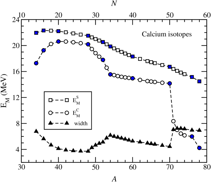
Figure 1: (Color online) Excitation energies of the isoscalar giant monopole resonance in the isotopic chain of calcium from scaling (squares) and constrained (circles) calculations as function of the mass number. The estimate of the resonance width (filled triangles) from Eq. (26) is also displayed.

In Figure 1 we display the scaled ($E_{M}^{S}$) and constrained ($E_{M}^{C}$) estimates of the average excitation energy of the monopole oscillation as a function of the mass number $A$ from the proton to the neutron drip lines. In this figure, the filled symbols correspond to closed subshell nuclei, whereas the open symbols correspond to open shell nuclei populated according to the uniform filling approximation. The predicted scaled and constrained energies of these open shell nuclei are thus for orientation purposes. Along the Ca chain the scaled monopole energies decrease rather smoothly when the number of neutrons moves from the stable nuclei towards the neutron drip line. The constrained energies also show a similar global tendency. However, two important differences can be observed as compared with the scaled energies. On the one hand, the reduction of $E^{C}_{M}$ near the neutron drip line is more pronounced than that in the case of scaled energies. The constrained energies $E^{C}_{M}$ also decrease for the proton rich members of the chain while for these nuclei the scaled energies $E^{S}_{M}$ remain close to the corresponding values in stable nuclei. On the other hand, relatively strong changes of the constrained energies can be observed at some subshell closures, in particular for the ones corresponding to neutron numbers $N=32$ and $N=34$ which are reached once the orbits $2p_{3/2}$ and $2p_{1/2}$ are completely filled. The resonance width along the chain, estimated with Eq. (26) is also displayed in Figure 1. It increases near the neutron and proton drip lines but also shows noticeable oscillations due to the shell effects at $N=32$ and $N=34$ in the middle of the Ca chain far from the drip lines.

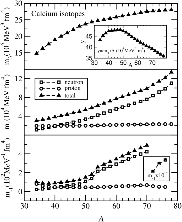
Figure 2: The $m_{3}$ sum rule for calcium isotopes as a function of the mass number $A$ is shown in the upper panel. The total $m_{1}$ and $m_{-1}$ sum rules (filled triangles) alongwith the contributions coming from neutrons (squares) and protons (circles) are displayed in the middle and lower panels.

The upper panel of Figure 2 displays the $m_{3}$ sum rule as a function of the mass number $A$ along the chain of Ca isotopes. From this figure, it can be seen that $m_{3}$ smoothly grows with increasing $A$ due to the global character of this sum rule [see Eq. (20)]. More interesting is the sum rule $m_{3}$ divided by $A$, which is shown in the inset of the same panel. The ratio $m_{3}/A$ is roughly constant for the stable nuclei and smoothly decreases when approaching the neutron and proton drip lines. This behavior can be understood in terms of the finite nucleus incompressibility $K_{A}$ R10 which is proportional to $m_{3}/A$. The value of $K_{A}$ can also be estimated through its leptodermous expansion R10 :

$$K_{A}=K_{\infty}+K_{sf}A^{-1/3}+K_{vs}I^{2}+K_{coul}Z^{2}A^{-4/3}+\ldots,$$ (27)

where $K_{\infty}$ is the nuclear matter incompressibility and $K_{sf}$, $K_{vs}$, and $K_{coul}$ are the surface, symmetry, and Coulomb corrections which in the scaling model are negative R10 . Near the neutron drip line, the surface ($K_{sf}A^{-1/3}$) and Coulomb ($K_{coul}Z^{2}A^{-4/3}$) terms decrease in absolute magnitude and tend to make $K_{A}$ larger with growing $A$, but the contribution of the symmetry term ($K_{vs}I^{2}$) dominates due to the large values of the neutron excess $I=(N-Z)/A$ and, in total, the finite nucleus incompressibility $K_{A}$ is reduced. Near the proton drip line, all of the three correction terms to $K_{A}$ are larger in absolute magnitude than those for stable nuclei, and thus the finite nucleus incompressibility again decreases. However, this effect near the proton drip line is smaller than that near the neutron drip line due to the smaller $|I|$ values, at least in the case of the Ca isotopes.

In the middle panel of Figure 2 we display the $m_{1}$ RPA sum rule for the chain of Ca isotopes as well as their contribution coming separately from protons and neutrons. As can be seen, the proton contribution to $m_{1}$ is roughly constant due to the fact that the proton rms radius only changes very little along the whole chain. Contrarily, the neutron contribution to $m_{1}$ increases almost linearly with increasing number of neutrons from the proton drip line up to ⁷⁰Ca from where it starts to grow faster following the trend of the rms radius of the neutron densities near the neutron drip line. Due to this behavior of the proton and neutron contributions, the full $m_{1}$ as a function of $A$ behaves almost as its neutron contribution along the chain. It should be pointed out that near the proton drip line the proton and neutron contributions are rather similar and both contribute equally to $m_{1}$, while near the neutron drip line the $m_{1}$ sum rule is basically given by its neutron contribution.

The $m_{-1}$ sum rule for the chain of Ca isotopes is displayed in the lower panel of Figure 2 together with their proton and neutron contributions. From this figure, one can see that the neutron contribution to $m_{-1}$ increases almost linearly with the mass number $A$ from the proton drip line till ⁴⁸Ca and from ⁵⁴Ca to ⁷⁰Ca with sudden changes from ⁴⁸Ca to ⁵⁴Ca and from ⁷⁰Ca up to the neutron drip line nucleus ⁷⁶Ca (shown in the inset). In contrast, the proton contribution to $m_{-1}$ remains roughly constant except from ⁴⁰Ca to the proton drip line (³⁴Ca) where it slightly increases. This behavior of the $m_{-1}$ sum rule together with the one exhibited by $m_{1}$ sum rule discussed previously, explains the global trends shown by the constrained average energy $E^{C}_{M}$ of the ISGMR along the Ca chain displayed in Figure 1 from the proton to the neutron drip lines.

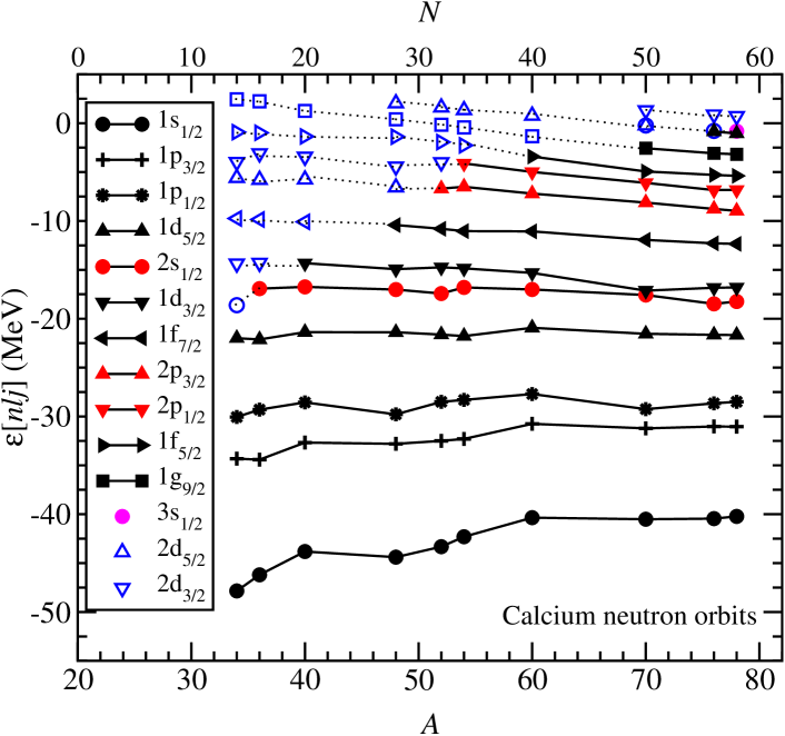
Figure 4: (Color online) Neutron single-particle energies for calcium isotopes as a function of $A$. Symbols joined by the dotted lines correspond to empty levels.

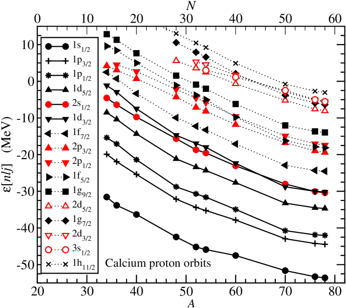
Figure 5: (Color online) Same as Figure 4 but for protons.

To obtain more insight about the neutron contribution to the $m_{1}$ and $m_{-1}$ sum rules we display in Figure 3 the mean square radius of each neutron orbit $nlj$ entering in the HF wave function of the ground state of the Ca nuclei along the isotopic chain. They can be contrasted with the neutron mean square radii of the same nuclei, shown by the thick horizontal lines. To help the discussion and for further purposes, the neutron and proton single-particle energy levels of the Ca isotopes are displayed in Figures 4 and 5 respectively. In these figures we have also included some quasi-bound levels owing to the centrifugal (neutrons) or centrifugal plus Coulomb (protons) barriers which simulate possible positive energy single-particle resonant states. From Figure 3 it can be seen that the deeper orbits almost give the same mean square radius along the whole isotopic chain in agreement with the fact that the more bound energy levels do not change very much from the proton to the neutron drip line (see Figure 4). Beyond ⁴⁸Ca, neutrons start to get accommodated in levels whose binding energies are relatively small and consequently the rms radii of the corresponding orbits increase. It is important to note that, in particular, the $2p_{3/2}$ and $2p_{1/2}$ orbits have a very large mean square radius in spite of the fact that their binding energies are not very small specially for the heaviest isotopes. The mean square radius of these $p$ orbits is larger than the one corresponding to the less bound level $1f_{5/2}$ and the one of the $2p_{1/2}$ orbit is similar to the one of the $1g_{9/2}$ orbit which lies higher in the energy spectrum. Near the neutron drip line, the very lightly bound level $2d_{5/2}$ is occupied and its wave function extends rather further increasing substantially the mean square radius of ⁷⁶Ca (the contribution of the $2d_{5/2}$ level to the mean square radius is shown by a triangle in the Figure 3 in the reduced scale as indicated). This fact produces a noticeable departure of the linear behavior exhibited by the $m_{1}$ sum rule near the neutron drip line.

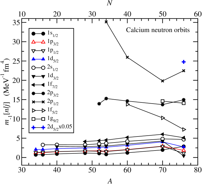
Figure 6: (Color online) Contributions of a single neutron in each occupied orbit to the $m_{-1}$ sum rule for the calcium isotopes.

In Figure 6 we display the contributions $m_{-1}[nlj]$ of a single nucleon in the occupied neutron orbits to the total $m_{-1}$ sum rule for each Ca isotope. From this figure one can see that the more bound neutron levels give almost the same single-particle contribution to $m_{-1}$ in all the nuclei of the Ca chain. The behavior of the $m_{-1}$ sum rule from ⁴⁸Ca onwards to the neutron drip line is governed by the outer orbits $2p_{3/2}$, $2p_{1/2}$, $1f_{5/2}$, $1g_{9/2}$ and $2d_{5/2}$ which give the largest contribution to $m_{-1}$ from ⁵²Ca to ⁷⁶Ca. The single-particle contributions to $m_{-1}$ from the orbits $2p_{3/2}$ and $1g_{9/2}$ are still roughly constant, however, strong changes can be observed in $m_{-1}[nlj]$ for the $2p_{1/2}$ and $1f_{5/2}$ orbits. A very large $m_{-1}[nlj]$ value comes from the outermost very lightly bound orbital $2d_{5/2}$ in the drip line nucleus ⁷⁶Ca (shown as a plus sign in the Figure in the reduced scale as indicated). The large single-particle contribution of the $2p_{1/2}$ and $2d_{5/2}$ orbits to $m_{-1}$ is due to the extension of their corresponding wave functions beyond the core of the nucleus, so that neutrons in such orbitals are much softer to pick up than neutrons accommodated in inner orbitals producing the strong enhancement of the total $m_{-1}$ sum rule.

Let us now discuss the enhancement of the $m_{-1}$ sum rule near the proton drip line. As it is known R17a , the depth of the proton single particle-potential for protons decreases when the number of neutrons in a isotopic chain decreases. Thus the outermost bound proton levels for nuclei near the proton drip line (see Figure 5) have little binding energy, their corresponding HF wave functions extend far from the core of the nuclei and consequently protons in these orbits are softer against pick-up increasing the contribution to the total $m_{-1}$ sum rule. This is just the case of the $1d_{3/2}$ orbit for protons in Ca isotopes (see Figure 5), which passes from $-7.5$ MeV in ⁴⁰Ca to $-1.1$ MeV in the proton drip line nucleus ³⁴Ca and gives the largest contribution to $m_{-1}$ in this case.

III.2 Connection with the RPA strength function

As mentioned, the sum rules $m_{1}$, $m_{3}$, and $m_{-1}$ computed from the HF ground state by means of Eqs. (9), (20), and (24), are the exact 1p-1h RPA value R11 . Actually, the self-consistent HF sum rules provide a practical means to check the accuracy of an RPA calculation of the strength function $S(E)$, provided that both the sum rule and the RPA calculation are performed in the same conditions. However, because of their complexity, it often happens that the RPA calculations are not fully self-consistent. For instance, the Coulomb and/or spin-orbit residual interactions may be absent in the RPA response. It has been recently shown AS that when the RPA calculations are performed self-consistently, the sum rules extracted from the RPA strength function are quite close to the values obtained in the HF sum rule approach.

RPA calculations for ³⁴Ca and ⁶⁰Ca were carried out some time ago R15 . The extracted ISGMR mean energies were $E^{S}_{M}=22.5$ MeV and $E^{C}_{M}=17.8$ MeV for ³⁴Ca, and $E^{S}_{M}=18.8$ MeV and $E^{C}_{M}=15.4$ MeV for ⁶⁰Ca. Although there are some differences, they compare well with the values from our sum rule calculation: $E^{S}_{M}=22.0$ MeV and $E^{C}_{M}=17.3$ MeV for ³⁴Ca, and $E^{S}_{M}=18.3$ MeV and $E^{C}_{M}=15.0$ MeV for ⁶⁰Ca. Our values for the resonance widths are 6.8 MeV in ³⁴Ca and 5.3 MeV in ⁶⁰Ca, which coincide with the RPA values obtained in Ref. R15 . The systematic deviation of about 0.5 MeV of the RPA average energies reported in Ref. R15 from our sum rule results may possibly be attributed to a deficiency in full self-consistency.

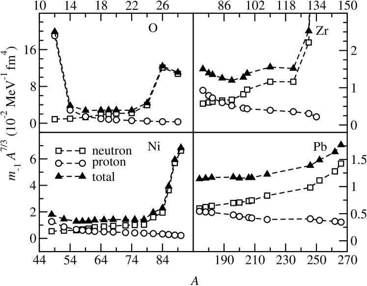
Figure 10: The $m_{-1}$ sum rule scaled by $A^{-7/3}$ is displayed for the isotopic chains of O, Ni, Zr, and Pb. The neutron (squares) and proton (circles) contributions to the total $m_{-1}$ are also plotted.

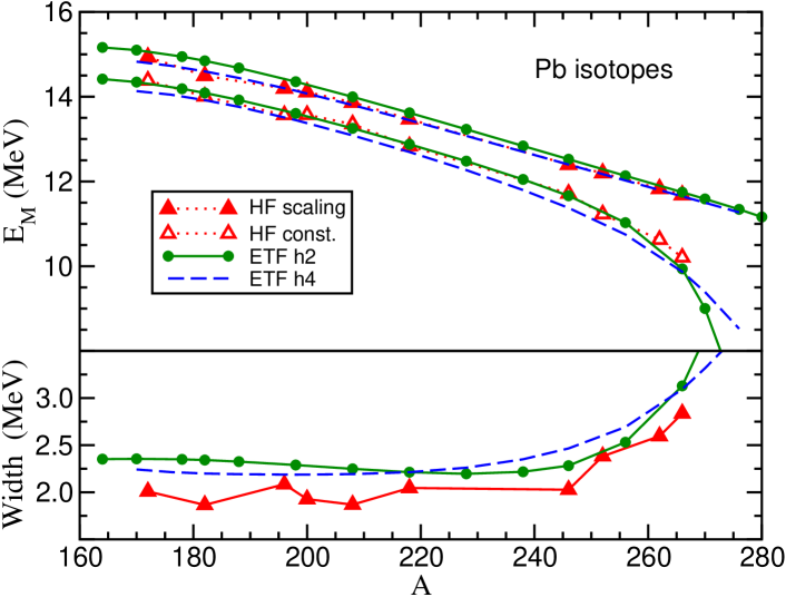
Figure 12: (Color online) Same as Figure 11 but for Pb isotopes.

The information contained in the energy spectra of the nuclei as well as in the values of the sum rules allows one to infer important properties of the strength function $S(E)$. Looking at Figure 10 of Ref. R15 , one can see that for ³⁴Ca there is a low energy bump in the region around 5–13 MeV. It is mainly due to transitions from the less bound proton levels ($1d_{3/2}$ and $2s_{1/2}$) to the continuum. These transitions enhance the $m_{-1}$ sum rule that weighs the low energy part of $S(E)$. The peak seen at high energies, in the 19–25 MeV region, receives contributions from the $1p\rightarrow 2p$ (resonant) transition of protons as well as from the $1p\rightarrow 2p$ and $1s\rightarrow 2s$ transitions of neutrons. Concerning ⁶⁰Ca (Figure 12 of Ref. R15 ), the low energy bump around 4–12 MeV is again mainly related to transitions to the continuum from the less bound levels, which in this case are due to neutrons. For this nucleus the last neutron in the $1f_{5/2}$ orbit is bound by 3.4 MeV which is in agreement with the threshold energy. The high energy peaks around 17 MeV and 21 MeV can be related to the $2s\rightarrow 3s$ (virtual) and to the $1d_{5/2}\rightarrow 2d_{5/2}$ (resonant) transitions for protons and to the $1p\rightarrow 2p$, $1d_{5/2}\rightarrow 2d_{5/2}$ and $1d_{3/2}\rightarrow 2d_{3/2}$ (resonant) transitions for neutrons. It should be pointed out that these transitions between single-particle levels, strictly speaking, should be related to peaks of the unperturbed strength, but they also appear when the RPA correlations are included. They are, however, slightly shifted to lower energies in general. With this experience in hand, we discuss from a qualitative point of view the most important trends of the RPA monopole response which can be expected for some representative nuclei of the Ca isotopic chain.

For ⁵²Ca and ⁵⁴Ca, a low energy bump in $S(E)$ starts to be developed due to transitions from $2p_{3/2}$ and $2p_{1/2}$ levels to the continuum. Although the strength in the low energy region of $S(E)$ should be small due to the relatively large binding energy of the last filled levels of neutrons of these nuclei (6.7 MeV and 4.1 MeV for ⁵²Ca and ⁵⁴Ca respectively), the large rms radii of these orbits favor a large overlap between the wave functions of these bound levels and the levels in the continuum R17b which increases the strength at these energies. This fact is supported, on average, by the enhancement of the $m_{-1}$ sum rule in passing from ⁴⁸Ca to ⁵⁴Ca. This confirms our assumption about the key role of the $2p_{3/2}$ and $2p_{1/2}$ orbits on the sudden increase of $m_{-1}$. In passing from ⁶⁰Ca to ⁷⁰Ca, the increase of $m_{1}$ and $m_{-1}$ is basically a size effect which explains the almost similar values of $E^{C}_{M}$ in both nuclei. Here one should also expect a low energy bump shifted towards lower energies due to transitions to the continuum from the $1g_{9/2}$ orbit which is bound by 2.5 MeV. For ⁷⁶Ca, $m_{-1}$ strongly increases due to the effect of the $2d_{5/2}$ orbit (bound by only 0.84 MeV) which has a very large rms radius. Although $m_{1}$ slightly increases, the large change of $m_{-1}$ explains the dramatic reduction of $E^{C}_{M}$ at the neutron drip line for the Ca isotopes. For this nucleus one could also expect a large low energy bump dominated by the transition to the continuum from the $2d_{5/2}$ level. The structure in $S(E)$ should also contain broad high energy peaks due to transitions from the deeply bound states to the unoccupied bound or resonant levels, coming from both neutrons and protons. From this it appears that the knowledge of the spectrum of a nucleus as well as the $m_{1}$ and $m_{-1}$ sum rules can provide useful information that allows one to sketch the behavior of the strength distribution $S(E)$.

III.3 Transition densities

In this subsection we will discuss the two following transition densities R13 :

$${\delta\rho}_{+1}(\mbox{\boldmath$r$})=-\frac{1}{2A\langle r^{2}\rangle}\big{[}3\rho(\mbox{\boldmath$r$})+r\rho^{\prime}(\mbox{\boldmath$r$})\big{]}$$ (28)

which is the Tassie transition density corresponding to the scaling transformation and

$${\delta\rho}_{-1}(\mbox{\boldmath$r$})=-\frac{1}{2m_{-1}}\left.\frac{\partial\rho_{\eta}(\mbox{\boldmath$r$})}{\partial\eta}\right|_{\eta=0}$$ (29)

which is the transition density in the constrained case. In Eq. (28) $\rho(\mbox{\boldmath$r$})$ is the ground-state particle density and $\langle r^{2}\rangle$ the mean square radius of the nucleus. In Eq. (29) $\rho_{\eta}(\mbox{\boldmath$r$})$ is the particle density built up with the HF single-particle wave functions that are solutions of the constrained Hamiltonian (23) and $m_{-1}$ is the inverse energy weighted sum rule calculated using (24). With the chosen normalization in Eqs. (28) and (29), it is ensured that when a single state exhausts the sum rule, then ${\delta\rho}_{+1}(\mbox{\boldmath$r$})={\delta\rho}_{-1}(\mbox{\boldmath$r$})$.

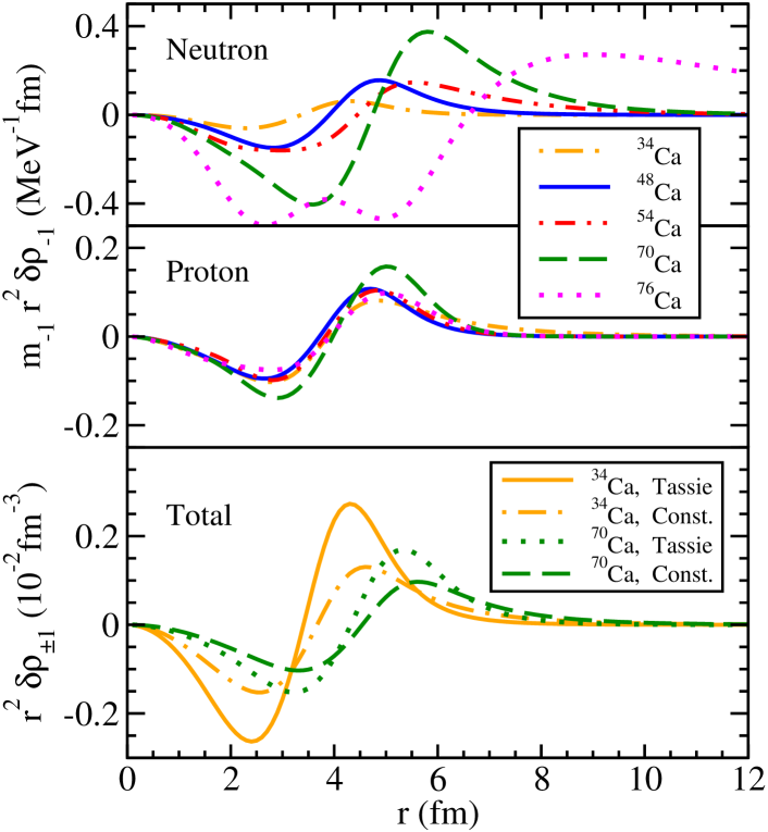
Figure 7: (Color online) Spatial variation of the constrained transition densities for neutrons (upper panel) and protons (middle panel) of some selected Ca isotopes. The Tassie and constrained transition densities are compared in the lower panel. Notice the different vertical scales.

Figure 7 displays the neutron (upper panel) and proton (middle panel) contributions to the constrained transition densities (29) multiplied by $r^{2}$ for some Ca isotopes between the proton and neutron drip lines, namely ³⁴Ca, ⁴⁸Ca, ⁵⁴Ca, ⁷⁰Ca and ⁷⁶Ca. The neutron contribution to $r^{2}{\delta\rho}_{-1}$ strongly depends on the neutron number of the considered isotope. The outer bump of the neutron contribution broadens and shifts to larger values of $r$ when the nuclei approach the neutron drip line; this is basically due to the neutrons in the outermost orbits which are loosely bound and extend very far from the center of the nucleus. For example, in Figure 7 one can see the effect of the $2p_{3/2}$ and $2p_{1/2}$ orbits in ⁵⁴Ca where the outer bump is clearly shifted with respect to that of the ⁴⁸Ca nucleus. The fact that the rms radius of the $1f_{5/2}$ and $1g_{9/2}$ orbits are similar to the ones of the $2p_{3/2}$ and $2p_{1/2}$ orbits (see Figure 3), is also reflected in the transition density of the nucleus ⁷⁰Ca whose external bump is located, roughly, at the same position as that of the one corresponding to ⁵⁴Ca. The very lightly bound $2d_{5/2}$ orbit has a very large rms radius (see Figure 3) and consequently the external bump of the neutron contribution to the constrained transition density is pushed to very large distances. The proton contribution to the constrained transition density displayed in the middle panel of Figure 7 shows a completely different pattern. On the one hand, both the inner and outer bumps are located approximately at the same positions for all the considered Ca isotopes, which is in agreement with the fact that the proton rms radius along a given isotopic chain remains approximately constant. On the other hand, the proton contribution to the total transition density decreases with increasing mass number . This is consistent with the fact that proton contributes proportionally less than neutrons to the $m_{-1}$ sum rule in neutron drip line nuclei as can be seen from the lower panel of Figure 2.

The lower panel of Figure 7 compares the Tassie and the constrained transition densities for the drip line nuclei ³⁴Ca and ⁷⁰Ca. For both nuclei the bumps of $r^{2}{\delta\rho}_{+1}$ and $r^{2}{\delta\rho}_{-1}$ are located at the same place. However, the shapes of both transition densities differ relatively between them. The strong fragmentation of the RPA strength in Ca isotopes, in particular in the drip line nuclei, can be gauged by the large enhancement of the resonance width in these nuclei (see Figure 1).

III.4 Other isotopic chains

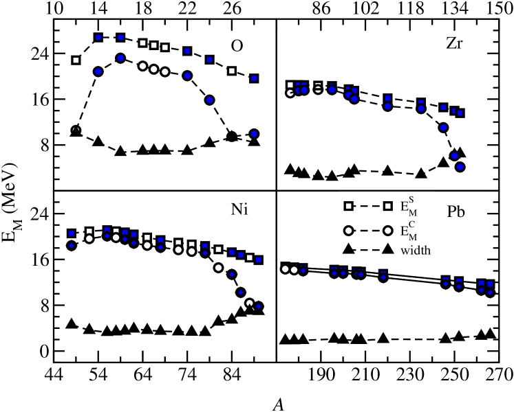
Figure 8: (Color online) Excitation energy of the ISGMR from scaling and constrained calculations alongwith the predicted resonance width for the isotopic chains of O, Ni, Zr, and Pb.

With the experience gained from this analysis of Ca isotopes, let us discuss the more salient features found in other isotopic chains. Figure 8 displays the scaled ($E^{S}_{M}$) and constrained ($E^{C}_{M}$) energies of the ISGMR as well as the resonance width for the O, Ni, Zr and Pb isotopic chains. The filled and open symbols correspond to subshell closed and open nuclei respectively. The scaled energies along these isotopic chains qualitatively behave in a similar way as those in Ca isotopes. In general, $E^{S}_{M}$ is roughly constant along the considered chains from the proton drip line to the stable nuclei and then shows a moderate downwards trend while approaching the neutron drip line. On the contrary, the constrained energies exhibit again a sizeable reduction near the neutron drip line and a moderate decrease near the proton drip line. One exception to this general behavior is ¹²O which shows a noticeable decrease of the scaled and constrained energies at the proton drip line. The reasons are similar to those discussed in the case of the ³⁴Ca, but more accentuated because of the smaller nuclear charge. Another exception is the heavy Pb chain where the constrained energy $E^{C}_{M}$ smoothly diminishes from the proton to the neutron drip lines showing a similar behavior to that of the scaled energy for these isotopes. As a consequence, for light and medium isotopic chains (O, Ni and Zr) the ISGMR width shows an enhancement near the proton and neutron drip lines (somewhat more pronounced at the neutron drip line), whereas the resonance widths for the Pb isotopes remain approximately constant along the whole chain. Thus, the resonance width in the different isotopic chains shows a downwards tendency with increasing atomic number, which suggests a smaller fragmentation and a more collective character in the ISGMR of heavy nuclei such as the Pb isotopes.

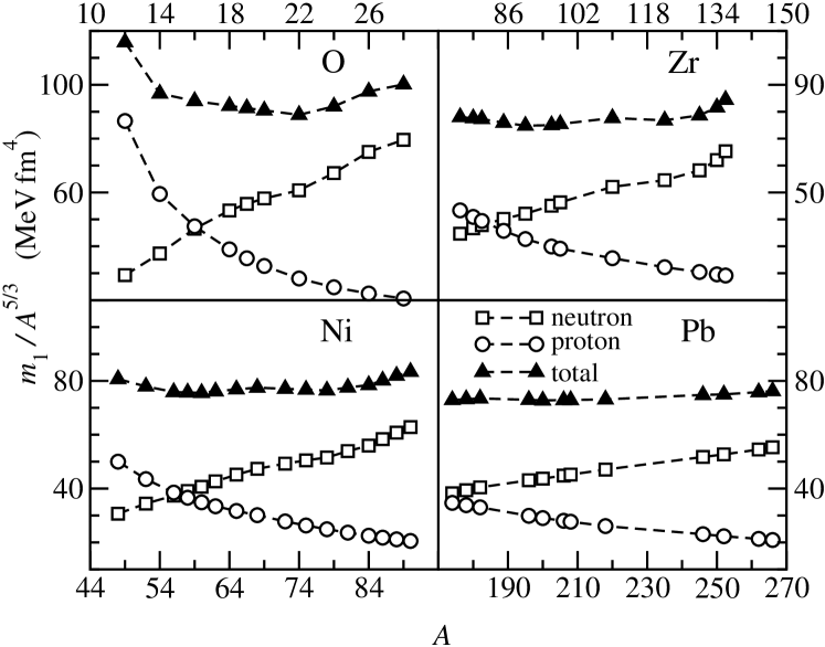
Figure 9: The $m_{1}$ sum rule scaled by $A^{-5/3}$ is displayed for the isotopic chains of O, Ni, Zr, and Pb. The neutron (squares) and proton (circles) contributions to the total $m_{1}$ are also plotted.

We now discuss the $m_{1}$ and $m_{-1}$ sum rules in O, Ni, Zr and Pb isotopes. In Figures 9 and 10 we display $m_{1}/A^{5/3}$ and $m_{-1}/A^{7/3}$, respectively, for the aforementioned isotopic chains. The scaling factors $A^{-5/3}$ and $A^{-7/3}$ remove the size dependence of the total $m_{1}$ and $m_{-1}$ sum rules R25 . From Figure 9 it can be seen that the neutron contribution to $m_{1}/A^{5/3}$ increases and the proton contribution decreases with growing mass number $A$. However, the total $m_{1}/A^{5/3}$ shows a rather constant behavior as a function of $A$ for all the considered isotopic chains, except maybe for some drip line nuclei. This means that the enhancement of the $m_{1}$ sum rule with $A$ displayed in Figure 2 for Ca isotopes up to ⁷⁰Ca is basically due to a size effect except near the drip line nuclei. The $A$-scaled $m_{-1}/A^{7/3}$ sum rule displayed in Figure 10 for the O, Ni, Zr and Pb chains shows a rather constant behavior in the region of stable nuclei. It clearly increases near the neutron drip lines and also for the proton drip line of oxygen. It shows the softness against pick-up of the nucleons from the outermost lightly bound levels thus giving the large enhancement of the $m_{-1}$ sum rule in the case of drip line nuclei.

From the sum rule approach we can also obtain some information about the RPA strength distributions for O, Ni, Zr, and Pb isotopes. In Ref. R25a the isoscalar monopole RPA strength for the neutron drip line nucleus ²⁸O was studied. We can analyze this nucleus on the basis of the sum rule approach. To help the discussion, we report in Table 1 the neutron and proton single-particle energy levels (including the quasi-bound ones) as well as the mean square radius of each bound orbit for this nucleus obtained with the SkM^∗ force. In this case the last occupied neutron level ($1d_{3/2}$) is bound by only 1.8 MeV. As discussed in Ref. R25a , the RPA strength develops a low energy bump due to transitions to the continuum from the $1d_{5/2}$, $2s_{1/2}$, and $1d_{3/2}$ levels, and a high energy peak due to the neutron transition $1p_{3/2}\rightarrow 2p_{3/2}$ (resonant) and the proton transitions from the $1s_{1/2}$, $1p_{1/2}$, and $1p_{3/2}$ levels to the unoccupied (but bound) $2s_{1/2}$, $2p_{1/2}$, and $2p_{3/2}$ levels, respectively. This structure is actually encoded in the sum rule approach used here. Looking at Figure 10, a noticeable enhancement of the scaled $m_{-1}/A^{7/3}$ sum rule for ²⁸O can be seen in qualitative agreement with the large amount of strength in the low energy part of $S(E)$. To be more quantitative, we also report in Table 1 the contribution to $m_{-1}$ coming from a single neutron in each occupied orbit. The largest part of the $m_{-1}$ sum rule comes from contributions of the $1d_{3/2}$, $2s_{1/2}$ and $1d_{5/2}$ neutron levels, which are responsible for 74%, 11% and 8% of the total $m_{-1}$ sum rule (263.022 MeV^-1 fm⁴), respectively. On the other hand, using the $\langle r^{2}\rangle$ values reported in the same Table, it is found that the contribution of these neutron levels to the total $m_{1}$ sum rule (2.586 $\times$ 10⁴ MeV fm⁴) is 23%, 11% and 25%, pointing out again their relevance in the low energy part of $S(E)$.

The single-nucleon contributions to $\langle r^{2}\rangle$ and to the $m_{-1}$ sum rule reported in Table 1 can also provide another information about $S(E)$. The energy corresponding to the maximum of the unperturbed strength due to transitions of the outermost nucleons to the continuum can be estimated for each orbit as the square root of the ratio of their single nucleon contributions to $m_{1}[nlj]$ and $m_{-1}[nlj]$. From the values reported in Table 1, this estimate gives 5.6 MeV and 9.6 MeV for the $1d_{3/2}$ and $2s_{1/2}$ neutron levels, in qualitative agreement with the position of the maxima in the unperturbed strength displayed in Figure 1 of Ref. R25a .

For the Ni isotopes the situation is qualitatively similar to that found for the Ca isotopic chain, although there are some differences. First, the enhancement of the polarizability shown by Ca isotopes when the $2p_{3/2}$ and $2p_{1/2}$ orbits are occupied (⁵²Ca and ⁵⁴Ca respectively) is appreciably attenuated in the corresponding Ni isotopes (⁶⁰Ni and ⁶²Ni). This is due to the fact that for Ni isotopes the $1f_{7/2}$ orbit for protons is filled and thus neutrons occupying the $2p_{3/2}$ and $2p_{1/2}$ levels are more bound and have smaller rms radii, as compared with the corresponding Ca isotopes. They thus contribute less to the $m_{-1}$ sum rule as can be realized from Figure 10 where no significant enhancement of the scaled $m_{-1}/A^{7/3}$ sum rule is observed. Second, in Ca isotopes the strong enhancement of the $m_{-1}$ sum rule and a moderate rise in $m_{1}$ start to be appreciable once the $1g_{9/2}$ orbit has been occupied (which corresponds to ⁷⁰Ca) and the very lightly bound $2d_{5/2}$ level starts to be populated (see Figure 2). Something similar happens for Ni isotopes beyond ⁷⁸Ni where the $2d_{5/2}$, $3s_{1/2}$ and $2d_{3/2}$ orbits become slightly bound and contribute largely to the enhancement of the $m_{-1}$ (strong) and $m_{1}$ (moderate) sum rules producing the decrease of the constrained energy and the enhancement of the width of the ISGMR in nuclei between ⁷⁸Ni and the drip line nucleus ⁹⁰Ni. However, the single nucleon contribution to the $m_{1}$ and $m_{-1}$ sum rules critically depends on its binding energy and increases very fast when the binding energy approaches zero. In our uniform filling approach and using the SkM^∗ force, the last occupied level in the drip nucleus ⁷⁶Ca ($2d_{5/2}$) is bound by only 0.85 MeV while in the Ni drip nucleus ⁹⁰Ni the outermost levels $2d_{5/2}$, $3s_{1/2}$ and $2d_{3/2}$ are bound by 3.45, 2.26 and 1.09 MeV respectively. These differences in the binding energies of the last occupied levels explain why the decrease in the constrained energy and the enhancement of the width of the ISGMR is more important in the Ca isotopes than in the Ni isotopes near the neutron drip line.

We next discuss the chain of the Zr isotopes. For the ¹²²Zr nucleus where the neutron shell $N=82$ is closed, the binding energy of the last bound orbit ($1h_{9/2}$) is 5.01 MeV with the SkM^∗ force. Some neutron orbits belonging to the $N=126$ closed shell, namely the $2f_{7/2}$, $3p_{3/2}$ and $3p_{1/2}$ orbitals, become very lightly bound in the ¹³⁰Zr, ¹³⁴Zr and ¹³⁶Zr isotopes and thus increase largely the $m_{1}$ and $m_{-1}$ sum rules in these nuclei close to the neutron drip line. In the uniform filling approximation, such a scenario can be appreciated in Figures 9 and 10 from the departure from the roughly constant value of the $A$-scaled $m_{1}/A^{5/3}$ and $m_{-1}/A^{7/3}$ sum rules in subshell closed Zr isotopes beyond ¹²²Zr. The strong enhancement of the $m_{-1}$ sum rule combined with the moderate rise in the $m_{1}$ sum rule produces the dramatic decrease of the constrained energy $E^{C}_{M}$ and the large increase of the resonance width near the neutron drip line which can be observed in Figure 8.

The situation is different in the heavy Pb isotopic chain. In this case the neutron drip line is reached once the $N=184$ shell is completely occupied (the last filled orbit $3d_{3/2}$ is bound by 2.58 MeV). In the lighter Ca, Ni and Zr isotopic chains, the shell gap above the $N=50$ and $N=82$ closed shells is strongly reduced when approaching the neutron drip line (and even disappears in the case of the Ca isotopes R1e ) as compared to those of the stable nuclei of these chains. Due to this fact, in nuclei near the neutron drip line some levels of the next major shell can still be bound before reaching it. However, in neutron-rich Pb isotopes the shell closure at $N=184$ is more robust and there are no bound levels belonging to the next major shell in the neutron drip nucleus. The $A$-scaled $m_{1}/A^{5/3}$ sum rule is practically constant along the whole chain and $m_{-1}/A^{7/3}$ shows a moderate increasing tendency near the neutron drip line (see Figures 9 and 10). The combination of these two effects causes the constrained energy and the energy width of the ISGMR in Pb neutron rich isotopes vary only slightly as compared to the corresponding values in the stable nuclei of the chain which can be seen in Figure 8.

We have treated all nuclei in the spherical approximation. This is justified to a large extent because of the semi-magic character of the isotopic chains considered. However, some of the isotopes may happen to be deformed, specially in the Zr chain. Since more than two decades ago, there is experimental evidence BU ; GA that the isoscalar monopole strength in deformed nuclei shows an additional lower energy peak when compared to that of spherical nuclei. This is interpreted as an effect of the coupling between the ISGMR and the isoscalar giant quadrupole resonance in deformed nuclei that broadens and splits the ISGMR strength into two components YO ; IT . We believe that this effect may be enhanced in deformed isotopes away from the valley of stability, because the broader distribution of the resonance strengths near the drip lines possibly would contribute to an increase of the coupling between the two excitation modes.

IV Semiclassical Extended Thomas-Fermi calculations

As mentioned in the introduction, it is known that for stable nuclei semiclassical approximations of Thomas-Fermi (TF) type and its extensions (ETF) used together with the sum rule approach provide a good estimate of the ISGMR excitation energies at least for stable nuclei R23 ; R24 ; R25 ; R25a1 ; R25b1 . In this section we want to study whether these semiclassical approximations are also able to follow the average trend of the quantal results in regions away from the stability line.

To describe semiclassically (at TF or ETF levels) the ISGMR excitation energies with the scaling method, we shall calculate first the ground-state neutron and proton densities. This is done by replacing the quantal kinetic energy density $\tau=\sum_{i=1}^{A}{|\mbox{\boldmath$\nabla$}\phi_{i}|}^{2}$ by the semiclassical one at TF level $\tau_{TF}=\sum_{q=n,p}3/5{(3\pi^{2})}^{2/3}\rho_{q}^{5/3}$ or at ETF level including $\hbar^{2}$ or $\hbar^{4}$ corrections R23 ; R24 into the Skyrme energy density functional and then solving the variational Euler-Lagrange equations for the neutron and proton densities $\rho_{n}$ and $\rho_{p}$, respectively R24 . The ETF method introduces $\hbar^{2}$ ($\hbar^{4}$) corrections on top of the simple TF kinetic energy through an expansion of second (fourth) order gradients of the particle density which include non-local contributions coming from the spin-orbit potential and the effective mass. These $\hbar$ corrections modify the asymptotic behavior of the self-consistent solution of the energy density and give a semiclassical density profile which averages the shell oscillations of the quantal HF density in the bulk and reproduces its fall-off at the surface. When $\hbar^{4}$ corrections are taken into account, the semiclassical energy of the ground state becomes roughly similar to the one obtained using the more cumbersome Strutinsky average method R24 .

In the semiclassical approaches, the neutron (proton) drip line is reached when the neutron (proton) chemical potential vanishes. We have checked R29 that the neutron drip lines for Ca and Pb at TF level using the SkM^∗ force correspond to neutron numbers of 48 and 195 which are in reasonable agreement with the HF predictions (56 and 184 respectively). This fact points out that nuclei near the drip lines can be studied through semiclassical methods of the ETF type. If the TF or ETF densities are used to compute (19), the virial theorem is, of course, strictly fulfilled due to the self-consistency. The semiclassical sum rules $m_{3}$ and $m_{1}$, which are needed to obtain the excitation energy of the ISGMR in the scaling method, are calculated using again Eqs. (20) and (9) but with the semiclassical self-consistent neutron and proton densities instead of the HF ones.

As it happens in the quantal case, the excitation energy of the ISGMR can also be estimated semiclassically by performing TF or ETF constrained calculations. In this case one has to minimize the constrained semiclassical energy

$$\int d\mbox{\boldmath$r$}[{\cal H}_{TF,ETF}-\eta r^{2}\rho_{\eta}]=E(\eta)-\eta\int d\mbox{\boldmath$r$}r^{2}\rho_{\eta},$$ (30)

where the quantal kinetic energy has been replaced by the TF or ETF equivalents. In order to obtain the semiclassical $m_{-1}$ sum rule, use is made of Eq. (22) but replacing the HF expectation values by the semiclassical ones.

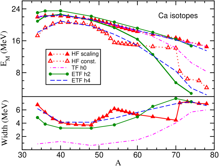
Figure 11: (Color online) The variation of the excitation energies of the isoscalar giant monopole resonance with the mass number $A$ for the Ca isotopic chain is shown in the upper panel. Semiclassical results of Thomas-Fermi (TF) type including $\hbar$ corrections at different orders, obtained with the scaling and constrained approaches, are contrasted with the RPA average energies. The resonance widths are presented in the lower panel.

Thus the semiclassical average excitation energies of the ISGMR are obtained from the RPA sum rules but with the HF expectation values entering in them replaced by the TF or ETF ones. The semiclassical excitation energies of the ISGMR calculated with the Skyrme SkM^∗ force using the scaling method and performing semiclassical constrained calculations are displayed in the upper panel of Figure 11 in comparison with the exact RPA average energies $\bar{E}_{3}=\sqrt{m_{3}/m_{1}}$ and $\bar{E}_{1}=\sqrt{m_{1}/m_{-1}}$ (which are the quantal scaled ($E^{S}_{M}$) and constrained ($E^{S}_{M}$) energies described in Section 2) along the Ca isotopic chain from the proton to the neutron drip lines. The semiclassical predictions of the excitation energies displayed in Figure 11 are calculated at pure TF level (dashed-dotted lines) and at ETF level including $\hbar^{2}$ (solid lines) and $\hbar^{4}$ (dashed lines) corrections. From this Figure it can be seen that the general trends of the excitation energies $\bar{E}_{3}$ of the ISGMR are well reproduced by all the considered semiclassical approximations along the whole isotopic chain. The agreement between the RPA $\bar{E}_{3}$ energies and their semiclassical counterpart improves by increasing the order of the $\hbar$-corrections as can be seen in the upper panel of Figure 11. If $\hbar^{4}$-corrections are included in the ETF calculation, then the RPA $\bar{E}_{3}$ energies are almost perfectly reproduced.

As far as the scaling approach is concerned, a first conclusion of this analysis is that the semiclassical approach to the RPA $\bar{E}_{3}$ (scaling) energies of the ISGMR agrees very well with the corresponding quantal RPA values not only for stable nuclei but also for nuclei near the drip lines, specially if $\hbar^{4}$ corrections are included in the semiclassical calculation. This fact points out that the role of shell effects is almost negligible in the estimate of the average energy $\bar{E}_{3}$ of the ISGMR obtained from the $m_{3}$ and $m_{1}$ sum rules on the one hand, and it justifies the use of the liquid-drop like expansion of the finite nucleus incompressibility (27) along the full isotopic chain on the other hand.

However, the situation is different when the ISGMR excitation energy is estimated by performing constrained calculations. In this case the constrained TF calculations give excitation energies which lie very close to the values obtained with the scaling method for Ca isotopes and thus fail in reproducing the RPA $\bar{E}_{1}$ energies in nuclei far from stability. Consequently, in the simple TF approximation, the predicted resonance width is very small and cannot reproduce the behavior of the RPA estimates of the width (26) along the chain as it can be seen in the lower panel of Figure 11, where the RPA widths and their semiclassical equivalents are displayed. The agreement between the RPA average energies $\bar{E}_{1}$ and their semiclassical estimates considerably improves when $\hbar$ corrections are considered explicitly in the calculation of the semiclassical densities. The ETF-$\hbar^{2}$ average energy of the ISGMR obtained by semiclassical constrained calculations qualitatively describes the behavior of the RPA results. A more quantitative agreement, at least from the proton drip to stable nuclei, is found when the average excitation energies are obtained through ETF-$\hbar^{4}$ calculations. Of course, the effects induced by some specific orbitals in the RPA $\bar{E}_{1}$ energies in Ca isotopes cannot be recovered by the semiclassical approaches. However, they nicely average the RPA results, the average being better when the $\hbar^{4}$-corrections are taken into account in the calculation. A similar situation is found in the estimates of the width of the ISGMR resonance along the isotopic chain, where the semiclassical approaches average again the RPA values as it can be seen in the lower panel of Figure 11.

A comparison between the RPA average excitation energies $\bar{E}_{3}$ and $\bar{E}_{1}$ and their semiclassical estimates is displayed in Figure 12 for the Pb isotopic chain. As it happens for Ca isotopes, the semiclassical scaled energies vary smoothly with the mass number $A$ and reproduce quite well the RPA $\bar{E}_{3}$ average energies from the proton to the neutron drip lines, at least for the subshell closed isotopes displayed in the figure. For Pb isotopes, the RPA $\bar{E}_{1}$ average energies show a rather smooth decreasing tendency with increasing mass number $A$ which is enhanced near the neutron drip line. As it happens for Ca isotopes, the semiclassical TF constrained energies lie close to the scaled ones and are unable to describe the strong decreasing of $\bar{E}_{1}$ near the neutron drip line. However, when $\hbar$-corrections are added, the semiclassical ETF estimates nicely reproduce the RPA $\bar{E}_{1}$ average energies, specially if $\hbar^{4}$-corrections are taken into account. As has been discussed before, the ISGMR of Pb isotopes exhibit a much more collective behavior and single-particle effects are much less important than in Ca isotopes even near the drip lines. Thus it is not completely surprising that the semiclassical approximations of ETF type are able to reproduce accurately not only the $\bar{E}_{3}$ average energies but also the $\bar{E}_{1}$ ones.

V Summary and conclusions

In this paper we have analyzed the variation of average properties (mean energies and resonance widths) of the isoscalar giant monopole resonance along the isotopic chains between the proton and neutron drip line for nuclei with magic atomic number from O to Pb. These average energies are obtained within the RPA sum rule approach using the SkM^∗ interaction. For each nucleus we have calculated the RPA cubic ($m_{3}$) and inverse energy ($m_{-1}$) weighted sum rules. The $m_{3}$ sum rule is obtained by means of a scaling transformation of the self-consistent HF neutron and proton densities, while $m_{-1}$ is computed by performing constrained Hartree-Fock calculations. For a Skyrme force the energy-weighted sum rule $m_{1}$ which is required for evaluating the average energies, is simply proportional to the mean square radius of the Hartree-Fock particle density.

The scaled energies $\bar{E}_{3}$ along the isotopic chains show general trends which are rather independent of the atomic number. The scaled estimate of the average excitation energy of the ISGMR shows a downwards tendency as one moves towards the neutron drip line from the stable nuclei. This fall-off of the scaled energy is smooth due to the moderate growing behavior of the $m_{3}$ sum rule with increasing mass number which is compensated by the stronger enhancement of the $m_{1}$ sum rule. The latter weighs more the tail of the density distributions and consequently is more important in nuclei near the neutron drip line. This reduction of the scaled estimate of the ISGMR average excitation energy at the neutron drip line is more noticeable in small and medium mass nuclei and its relative importance decreases with increasing atomic number.

A similar decreasing tendency of $\bar{E}_{3}$ near the proton drip line appears only for very light nuclei such as the O isotopes, and it is not observed in heavier systems. The reason lies in the fact that for proton-drip line nuclei, the Coulomb barrier prevents their single-particle wave functions from extending much from the center of the nucleus, thus prohibiting an enhancement of the rms radius of the density which in turn would reduce the scaled average excitation energies of these nuclei. Due to the global character of the scaled estimate of the ISGMR average energies that depend on the nuclear densities, single-particle effects play a minor role on these energies even for drip line nuclei. In this regard, the macroscopic description of the finite nucleus incompressibility based on a leptodermous expansion is still valid and allows for a qualitative understanding of the behavior of the scaled estimates of the ISGMR average energies even near the drip lines.

The global behavior of the average energies of the ISGMR estimated through constrained calculations is, in general, similar to the one exhibited by the scaled energies. These average energies are in general smaller in drip line nuclei than those in stable ones. The effect is much more pronounced for the constrained energies calculated near the neutron drip line, in contrast to those calculated in the scaling approximation. Near the neutron drip line the constrained estimate of excitation energy of the ISGMR clearly deviates from the empirical $A^{-1/3}$ law known for stable nuclei. The reason for this behavior of the constrained estimate near the drip lines is due to the fact that the single-particle effects are much more important in this case than in the scaling calculation. Nuclei near the drip lines are characterized by neutrons (protons) occupying very lightly bound levels whose corresponding wave functions extend very far from the core of the nucleus, specially in the case of neutron rich nuclei owing to the absence of Coulomb barrier. Neutrons occupying these orbits have larger single-particle neutron mean square radius and at the same time are much softer against pick-up than those filling more bound orbits. Consequently, both the energy and the inverse energy weighted sum rules are enhanced, this effect being more important in the latter than in the former. This explains the sizeable decrease of the constrained estimate of the average energy of the ISGMR in nuclei near the neutron drip lines. This effect is particularly important in the Ca and Zr isotopic chains where the corresponding neutron drip nuclei (⁷⁶Ca and ¹³⁶Zr respectively) have the last occupied orbit bound by less than 1 MeV. It should also be pointed out that for the particular nuclei ⁵²Ca and ⁵⁴Ca which are not neutron drip nuclei, we find a noticeable enhancement of the $m_{1}$ and $m_{-1}$ sum rules due to the fact that for these specific nuclei the neutron $2p_{3/2}$ and $2p_{1/2}$ single-particle wave functions extend very far from the core although their binding energies are not particularly small.

The RPA sum rule description of some of the average properties of the ISGMR has some clear limitations as compared with a full RPA calculation of the response function. Thus only some global trends of the RPA strength can be inferred from our calculation. For instance, the reduction of the scaled and constrained energies near the drip lines should be associated with the appearance of a noticeable RPA strength in the low energy region as suggested by the enhancement of the $m_{-1}$ sum rule. As in a full RPA calculation, nuclei near the drip lines are found to have a large resonance width in our approach, but the mean energy of the resonance cannot be determined very precisely because the scaled and constrained energies, which are upper and lower bounds of the mean energy, are largely separated. This large width near the drip lines can be due to a very broad resonance as well as to a fragmentation of the strength distribution.

We have also investigated the ability of semiclassical approximations of the TF type and its extensions including $\hbar$-corrections (ETF) for describing the ISGMR near the drip lines within the sum rule approach. The semiclassical sum rules are obtained by using the full quantal RPA expressions but with the HF expectation values replaced by the semiclassical ones at the TF or the ETF levels. The semiclassical estimates of the average scaled and constrained energies are free from any shell effects. Thus some of the discussed trends, as for instance the enhancement of the $m_{1}$ and $m_{-1}$ sum rules when a particular orbital is occupied, are only taken into account on the average in the semiclassical description. This means that the quantal RPA scaled and constrained energies may be spread around the values provided by the semiclassical calculations. In nuclei near the drip lines the pure TF approximation fails in reproducing, even on the average, the global trends of the RPA constrained energies and thus the widths of the ISGMR, due to the poor description of the nuclear surface. However, when the $\hbar^{2}$-order corrections, and those of $\hbar^{4}$ order, are included in the semiclassical calculation, the ETF description of the surface of the nuclei agrees better with the HF one and the RPA scaled and constrained energies are nicely averaged by the corresponding semiclassical counterpart.

It is known that a right description of nuclei near the drip lines has to take into account pairing correlations, in particular for open shell nuclei. The inclusion of pairing in RPA, i.e. the quasiparticle RPA, has a noticeable effect on the strength of the response of the drip line nuclei to external fields QRPA ; however its impact on the average excitation energies is much less. Thus, in the present approximation we did not consider pairing and assumed the uniform filling approach in order to obtain an insight into the general trends of the ISGMR in exotic nuclei near the drip lines. In a next step, the application of the sum rule approach in the quasiparticle RPA should be probed in order to properly take into account the influence of pairing correlations on the average properties of the ISGMR. Investigations in this direction are in progress.

Table 1: Neutron and proton single-particle energy levels (in MeV) with the occupancy (given within the round brackets) for ²⁸O. The mean square radius $\langle r^{2}\rangle$ (in fm²) and the single-nucleon contribution to the $m_{-1}$ sum rule of each orbital (in MeV^-1fm⁴) are also given.

Neutron State	Energy (n)	$\langle r^{2}\rangle$	$m_{-1}[nlj]$	Proton State	Energy (p)	$\langle r^{2}\rangle$	$m_{-1}[nlj]$
$1s_{1/2}$	$-31.920$ (1)	5.085	0.3093	$1s_{1/2}$	$-44.132$ (1)	5.433	0.3505
$1p_{3/2}$	$-19.920$ (1)	8.701	0.9664	$1p_{3/2}$	$-31.726$ (1)	8.786	1.0010
$1p_{1/2}$	$-14.936$ (1)	9.194	1.5875	$1p_{1/2}$	$-27.060$ (1)	9.068	1.3510
$1d_{5/2}$	$-8.641$ (1)	12.962	3.6757	$1d_{5/2}$	$-19.389$ (0)	—	—
$2s_{1/2}$	$-5.997$ (1)	16.689	15.1465	$2s_{1/2}$	$-15.143$ (0)	—	—
$1d_{3/2}$	$-1.780$ (1)	18.278	48.9019	$1d_{3/2}$	$-12.415$ (0)	—	—
$2p_{3/2}$	$0.526$ (0)	—	—	$1f_{7/2}$	$-6.665$ (0)	—	—
$1f_{7/2}$	$1.731$ (0)	—	—	$2p_{3/2}$	$-2.380$ (0)	—	—
$1g_{9/2}$	$10.366$ (0)	—	—	$2p_{1/2}$	$-0.701$ (0)	—	—

Figure 3: (Color online) Mean square radii of the neutron single-particle orbits for the isotopic chain of calcium as a function of the mass number. The horizontal bars depict the value of the total neutron mean square radius of each isotope.