Space- and time-like electromagnetic form factors of the nucleon

Abstract

Recent experimental data on space- and time-like form factors of the nucleon are analyzed in terms of a two-component model with a quark-like intrinsic structure and a meson cloud. A good overall agreement is found for all electromagnetic form factors with the exception of the neutron magnetic form factor in the time-like region.

PACS numbers: 13.40.Gp, 14.20.Dh

I Introduction

The structure of the nucleon is of fundamental importance in nuclear and particle physics. The electromagnetic form factors are key ingredients to the understanding of the internal structure of composite particles like the nucleon since they contain the information about the distributions of charge and magnetization. The first evidence that the nucleon is not a point particle but has an internal structure came from the measurement of the anomalous magnetic moment of the proton in the 1930’s stern , which was determined to be 2.5 times as large as one would expect for a spin $1/2$ Dirac particle (the actual value is 2.793). The finite size of the proton was measured in the 1950’s in electron scattering experiments at SLAC to be $\sim 0.8$ fm hofstadter (compared to the current value of 0.895 fm). The first evidence for point-like constituents (quarks) inside the proton was found in deep-inelastic-scattering experiments in the late 1960’s by the MIT-SLAC collaboration dis , which eventually together with many other developments would lead to the formulation of QCD in the 1970’s as the theory of strongly interacting particles.

The complex structure of the proton manifested itself once again in recent polarization transfer experiments jones ; gayou which showed that the ratio of electric and magnetic form factors of the proton exhibits a dramatically different behavior as a function of the momentum transfer as compared to the generally accepted picture of form factor scaling obtained from the Rosenbluth separation method walker ; andivahis . The discrepancy between the experimental results has been the subject of many theoretical investigations which have focussed on radiative corrections due to two-photon exchange processes twophoton ; tomasi .

The new experimental data for the proton form factor ratio are in excellent agreement with a phenomenological model of the nucleon put forward in 1973 IJL wherein the external photon couples both to an intrinsic structure and to a meson cloud through the intermediate vector mesons ($\rho$, $\omega$, and $\varphi$). The linear drop in the proton form factor ratio was also predicted in a chiral soliton model soliton before the polarization transfer data from Jefferson Lab became available in 2000 jones ; gayou . On the contrary, the new experimental data for the neutron madey are in agreement with the vector meson dominance (VMD) model of IJL for small values of $Q^{2}$, but not so for higher values of $Q^{2}$.

The aim of this contribution is to present an simultaneous study of all electromagnetic form factors of the nucleon not only in the space-like region where they can be measured in electron scattering experiments, but also in the time-like region where they can be studied through the creation or annihilation of a nucleon-antinucleon pair. The analysis is carried out in a modified version of IJL : a two-component model consisting of an intrinsic (three-quark) structure and a meson cloud whose effects are taken into account via vector meson dominance (VMD) couplings BI .

This manuscript is organized as follows: in Section 2 the experimental situation for the form factor ratio of the proton is reviewed briefly. The main ingredients of the two-component model of BI and its application to the space-like form factors are discussed in Section 3 and extended to the time-like region in Section 4. The last section contains the summary and conclusions.

II Electromagnetic form factors

Electromagnetic form factors provide important information on the structure of the nucleon. Relativistic invariance determines the form of the nucleon current for one-photon exchange to be

$$J_{\mu} = F_{1}(Q^{2})\,\gamma^{\mu}+\frac{1}{2M}F_{2}(Q^{2})\,i\sigma^{\mu\nu}q_{\nu}~{},$$ (1)

where $M$ denotes the nucleon mass, $q=(\omega,\vec{q})$ is the four-momentum of the virtual photon and $Q^{2}=-q^{2}$. $F_{1}$ denotes the Dirac form factor, and $F_{2}$ represents the helicity flip Pauli form factor which is proportional to the anomalous magnetic moment. The Sachs form factors, $G_{E}$ and $G_{M}$, can be obtained from $F_{1}$ and $F_{2}$ by the relations

$$G_{E}(Q^{2}) = F_{1}(Q^{2})-\tau F_{2}(Q^{2})~{},$$

$$G_{M}(Q^{2}) = F_{1}(Q^{2})+F_{2}(Q^{2})~{},$$ (2)

with $\tau=Q^{2}/4M^{2}$. $G_{E}$ and $G_{M}$ are the form factors describing the distribution of electric charge and magnetization as a function of the $Q^{2}$ satisfying

$$G_{E_{p/n}}(0) = e_{p/n}~{},$$

$$G_{M_{p/n}}(0) = \mu_{p/n}~{},$$ (3)

where $e_{p/n}$ and $\mu_{p/n}$ denote the electric charge and magnetic moment of the proton/neutron.

II.1 Rosenbluth separation method

The differential cross section for elastic electron-nucleon scattering is given by the Rosenbluth formula rosenbluth

$$\frac{d\sigma}{d\Omega} = \left(\frac{d\sigma}{d\Omega}\right)_{\rm Mott}\left[\frac{G_{E}^{2}+\tau G_{M}^{2}}{1+\tau}+2\tau G_{M}^{2}\tan^{2}\frac{\theta}{2}\right]$$ (4)

$$= \left(\frac{d\sigma}{d\Omega}\right)_{\rm Mott}\frac{\tau}{\epsilon(1+\tau)}\left[G_{M}^{2}+\frac{\epsilon}{\tau}G_{E}^{2}\right]~{},$$

where $\epsilon=1/[1+2(1+\tau)\tan^{2}(\theta/2)]$ is the linear polarization of the virtual photon and $\theta$ the scattering angle. For a point-like proton ($G_{E}=G_{M}=1$) this expression reduces to the differential cross section for electron scattering off a spin-$1/2$ Dirac particle. By measuring the differential cross section at a fixed value of $Q^{2}$ as a function of $\epsilon$ (or equivalently, as a function of the scattering angle $\theta$), the electric and magnetic form factors can be disentangled according to the Rosenbluth separation method. However, for large values of $Q^{2}$ the measured cross section is dominated by the magnetic form factor, which makes the determination of the electric form factor difficult due to an increasing systematic uncertainty with $Q^{2}$. The electric and magnetic form factors obtained with the Rosenbluth method can be described to a reasonable approximation (up to the 10-20 $\%$ level) by the so-called dipole fit bosted

$$G_{E_{p}}(Q^{2})\;\approx\;\frac{G_{M_{p}}(Q^{2})}{\mu_{p}}\;\approx\;\frac{G_{M_{n}}(Q^{2})}{\mu_{n}}\;\approx\;G_{D}(Q^{2})\;=\;\frac{1}{(1+Q^{2}/0.71)^{2}}~{}.$$ (5)

The electric form factor of the neutron is relatively small and was parametrized in 1971 by the the Galster formula

$$G_{E_{n}}(Q^{2})\;=\;-\mu_{n}\frac{a\tau}{1+b\tau}G_{D}(Q^{2})~{},$$ (6)

with $a=1$ and $b=5.6$ galster . In a more recent fit, the coefficients $a$ and $b$ were determined to be $a=0.888\pm 0.023$ and $b=3.21\pm 0.33$ madey .

II.2 Polarization transfer method

In recent years, experiments with polarized electron beams have become feasible at MIT-Bates, MAMI and Jefferson Lab. In polarization transfer experiments

$$\vec{e}+p\rightarrow e+\vec{p}~{},$$ (7)

the polarization of the recoiling proton is measured from which the ratio of the electric and magnetic form factors can be determined directly as

$$\frac{G_{E}}{G_{M}} = -\frac{P_{t}}{P_{l}}\frac{E+E^{\prime}}{2M_{p}}\tan\frac{\theta}{2}~{},$$ (8)

where $P_{t}$ and $P_{l}$ denote the polarization of the proton perpendicular and parallel to its momentum in the scattering plane. $E$ and $E^{\prime}$ denote the initial and final electron energy. The simultaneous measurement of the two polarization components greatly reduces the systematic uncertainties. The results of the polarization transfer method showed a big surprise. The ratio of electric and magnetic form factors of the proton dropped almost linearly with $Q^{2}$ jones ; gayou

$$R_{p}\;=\;\frac{\mu_{p}G_{E_{p}}(Q^{2})}{G_{M_{p}}(Q^{2})}\;\approx\;1-0.13(Q^{2}-0.29)~{},$$ (9)

in clear disagreement with the Rosenbluth results of Eq. (5) which correspond to a constant value of $R_{p}$

$$R_{p}\;\approx\;1~{}.$$ (10)

The vector meson dominance (VMD) model proposed in 1973 by Iachello, Jackson and Lande IJL is in excellent agreement with the new polarization transfer data, although for $G_{E_{p}}$ this model is in poor ageement with the SLAC data over the entire $Q^{2}$ range andivahis . Also Holzwarth predicted a linear drop in the proton form factor ratio soliton before the polarization transfer data from Jefferson Lab became available in 2000 jones ; gayou . Since then several theoretical calculations have reproduced this behavior review .

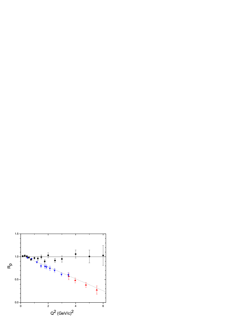
Figure 1: Comparison of the proton form factor ratio $R_{p}=\mu_{p}G_{E_{p}}/G_{M_{p}}$ obtained from the Rosenbluth separation method walker (filled circles) and from the polarization transfer method jones (filled inverted triangles) and gayou (filled triangles). The dotted and solid lines are calculated with Eqs. (9) and (10), respectively.

To illustrate the difference between the two methods, I show in Fig. 1 the proton form factor ratio $R_{p}$ obtained from the Rosenbluth separation technique walker and from the polarization transfer experiments jones ; gayou . In view of the observed discrepancy the old Rosenbluth data have been reanalyzed arrington and were found to be in agreement with form factor scaling of Eq. (10). In addition, new Rosenbluth experiments have been carried out recently at JLab Christy ; Qattan to try to settle the contradictory experimental results. Also in this case, the new results agree within error bars with those obtained earlier at SLAC walker . Theoretically, radiative corrections due to two-photon exchange processes are being investigated as a possible source of the observed differences twophoton ; tomasi . The importance of two-photon exchange processes can be tested experimentally by measuring the ratio of elastic electron and positron scattering off a proton vepp .

III Vector meson dominance

The first models to describe the electromagnetic form factors of the nucleon are based on vector meson dominance in which it is assumed that the photon couples to the nucleon through intermediary vector mesons with the same quantum numbers as the photon IJL ; hoehler ; gari ; lomon . In order to take into account the coupling to the vector mesons the proton and neutron electromagnetic form factors are expressed in terms of the isoscalar, $F^{S}$, and isovector, $F^{V}$, form factors as

$$G_{M_{p}} = \left(F_{1}^{S}+F_{1}^{V}\right)+\left(F_{2}^{S}+F_{2}^{V}\right)~{},$$

$$G_{E_{p}} = \left(F_{1}^{S}+F_{1}^{V}\right)-\tau\left(F_{2}^{S}+F_{2}^{V}\right)~{},$$

$$G_{M_{n}} = \left(F_{1}^{S}-F_{1}^{V}\right)+\left(F_{2}^{S}-F_{2}^{V}\right)~{},$$

$$G_{E_{n}} = \left(F_{1}^{S}-F_{1}^{V}\right)-\tau\left(F_{2}^{S}-F_{2}^{V}\right)~{}.$$ (11)

In the VMD calculation of 1973 IJL , the Dirac form factor was attributed to both the intrinsic structure and the meson cloud, and the Pauli form factor entirely to the meson cloud. Since this model was formulated previous to the development of QCD, no explicit reference was made to the nature of the intrinsic structure. In this contribution, the intrinsic structure is identified with a three valence quark structure. In particular, the question of whether or not there is a coupling to the intrinsic structure also in the Pauli form factor $F_{2}$ is studied. Relativistic constituent quark models in the light-front approach frank ; salme point to the occurrence of such a coupling. Dimensional counting rules count and the development of perturbative QCD (p-QCD) pqcd has put some constraints to the asymptotic behavior of the form factors, namely that the non-spin-flip form factor $F_{1}\rightarrow 1/Q^{4}$ and the spin-flip form factor $F_{2}\rightarrow 1/Q^{6}$. This behavior has been very recently confirmed in a perturbative QCD re-analysis belitsky ; brodsky . The 1973 parametrization, even if it was introduced before the development of p-QCD, had this behavior. In modifying it, we insist on maintaining the asymptotic behavior of p-QCD and introduce in $F_{2}^{V}$ a term of the type $g(Q^{2})/(1+\gamma Q^{2})$. These considerations lead to the following form of the isoscalar and isovector Dirac and Pauli form factors BI

$$F_{1}^{S}(Q^{2}) = \frac{1}{2}g(Q^{2})\left[1-\beta_{\omega}-\beta_{\varphi}+\beta_{\omega}\frac{m_{\omega}^{2}}{m_{\omega}^{2}+Q^{2}}+\beta_{\varphi}\frac{m_{\varphi}^{2}}{m_{\varphi}^{2}+Q^{2}}\right]~{},$$

$$F_{1}^{V}(Q^{2}) = \frac{1}{2}g(Q^{2})\left[1-\beta_{\rho}+\beta_{\rho}\frac{m_{\rho}^{2}}{m_{\rho}^{2}+Q^{2}}\right]~{},$$

$$F_{2}^{S}(Q^{2}) = \frac{1}{2}g(Q^{2})\left[\left(\mu_{p}+\mu_{n}-1-\alpha_{\varphi}\right)\frac{m_{\omega}^{2}}{m_{\omega}^{2}+Q^{2}}+\alpha_{\varphi}\frac{m_{\varphi}^{2}}{m_{\varphi}^{2}+Q^{2}}\right]~{},$$

$$F_{2}^{V}(Q^{2}) = \frac{1}{2}g(Q^{2})\left[\frac{(\mu_{p}-\mu_{n}-1-\alpha_{\rho})}{1+\gamma Q^{2}}+\alpha_{\rho}\frac{m_{\rho}^{2}}{m_{\rho}^{2}+Q^{2}}\right]~{},$$ (12)

with $\mu_{p}=2.793$ $\mu_{N}$ and $\mu_{n}=-1.913$ $\mu_{N}$. This parametrization insures that the three-quark contribution to the anomalous moment is purely isovector, as given by $SU(6)$. For the intrinsic form factor a dipole form $g(Q^{2})=(1+\gamma Q^{2})^{-2}$ is used which is consistent with p-QCD and in addition coincides with the form used in an algebraic treatment of the intrinsic three quark structure bijker . The values of the meson masses are the standard ones: $m_{\rho}=0.776$ GeV, $m_{\omega}=0.783$ GeV, $m_{\varphi}=1.019$ GeV.

The large width of the $\rho$ meson is crucial for the small $Q^{2}$ behavior of the form factors and is taken is taken into account in the same way as in IJL by the replacement frazer

$$\frac{m_{\rho}^{2}}{m_{\rho}^{2}+Q^{2}}\rightarrow\frac{m_{\rho}^{2}+8\Gamma_{\rho}m_{\pi}/\pi}{m_{\rho}^{2}+Q^{2}+\left(4m_{\pi}^{2}+Q^{2}\right)\Gamma_{\rho}\alpha(Q^{2})/m_{\pi}}~{},$$ (13)

with

$$\alpha\left(Q^{2}\right)=\frac{2}{\pi}\sqrt{\frac{4m_{\pi}^{2}+Q^{2}}{Q^{2}}}\,\ln\left(\frac{\sqrt{4m_{\pi}^{2}+Q^{2}}+\sqrt{Q^{2}}}{2m_{\pi}}\right)~{}.$$ (14)

For the effective width the same value is taken as in IJL ; wan : $\Gamma_{\rho}=0.112$ GeV. For small values of $Q^{2}$ the form factors are dominated by the meson dynamics, whereas for large values the modification from dimensional counting laws from perturbative QCD can be taken into account by scaling $Q^{2}$ with the strong coupling constant gari

$$Q^{2}\rightarrow Q^{2}\frac{\alpha_{s}(0)}{\alpha_{s}(Q^{2})}\;=\;Q^{2}\frac{\ln\left[\left(\Lambda^{2}+Q^{2}\right)/\Lambda_{\rm QCD}^{2}\right]}{\ln\left[\Lambda^{2}/\Lambda_{\rm QCD}^{2}\right]}~{}.$$ (15)

Since this modification is not very important for range of $Q^{2}$ values $0<Q^{2}<10$ GeV² considered in the present contribution, it will be neglected in the remainder.

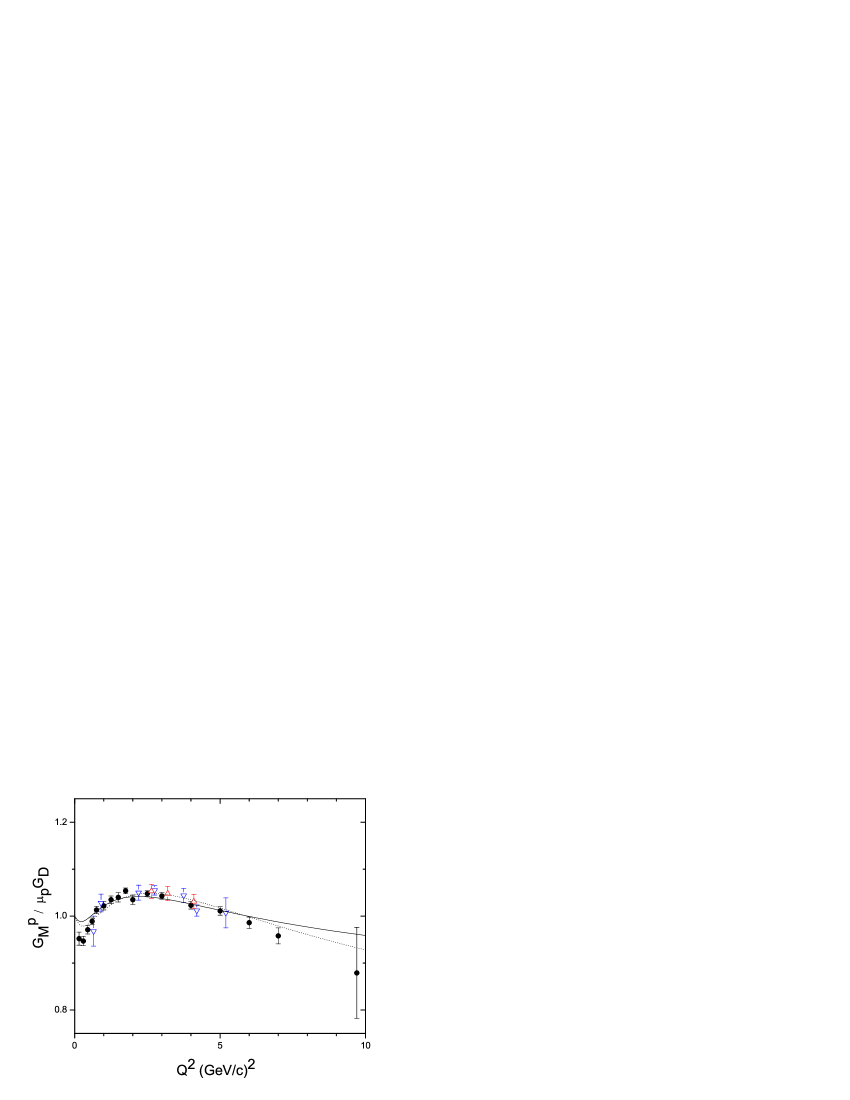
Figure 2: Comparison between the experimental and theoretical proton magnetic form factor $G_{M_{p}}/\mu_{p}G_{D}$ in the space-like region. The experimental data included in the fit are taken from walker (filled circles). Additional data, not included in the fit, are taken from Christy (open inverted triangles) and from Qattan (open triangles). The solid line is from the present calculation and the dotted line from IJL .

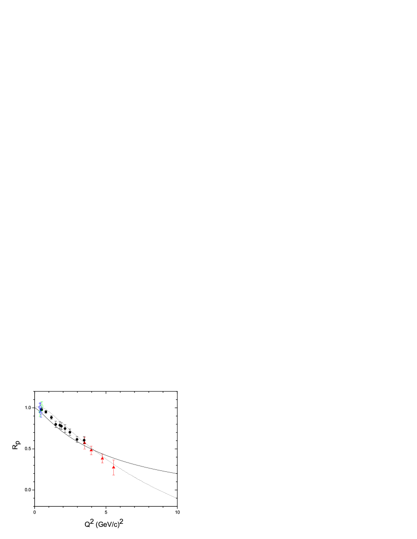
Figure 3: As Fig. 2, but for the proton form factor ratio $R_{p}=\mu_{p}G_{E_{p}}/G_{M_{p}}$. The experimental data included in the fit are taken from jones (filled circles) and gayou (filled triangles) Additional data, not included in the fit, are taken from milbrath (open squares) and pospi (open inverted triangles).

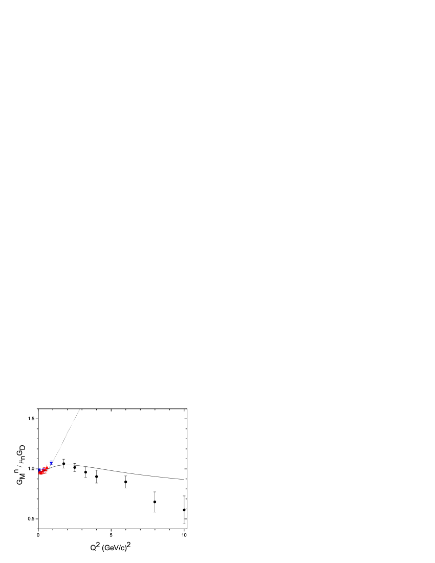
Figure 4: As Fig. 2, but for the neutron magnetic form factor $G_{M_{n}}/\mu_{n}G_{D}$. The experimental data included in the fit are taken from gmnfit : Rock & Lung (filled circles) and Xu (filled triangles) and Kubon (filled inverted triangles).

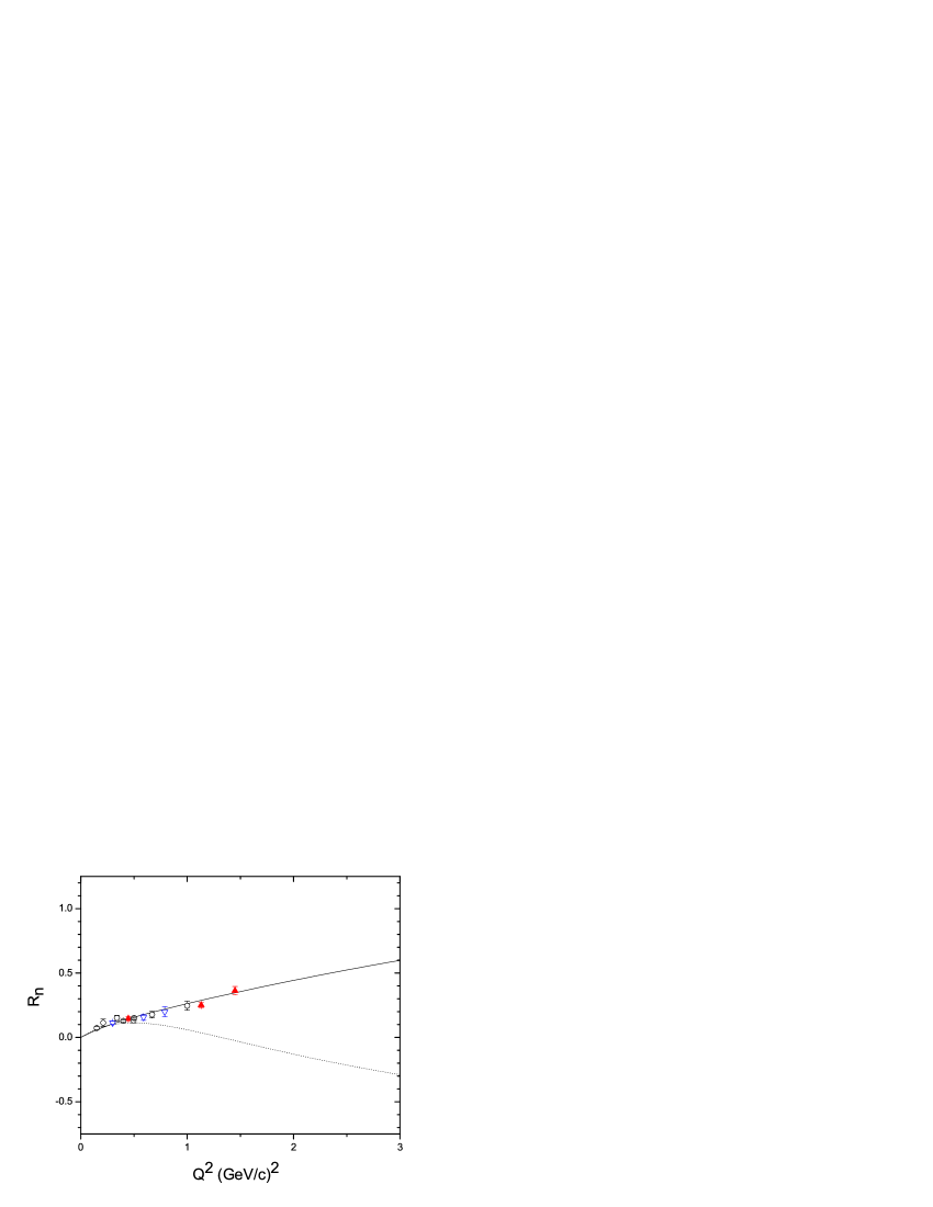
Figure 5: As Fig. 2, but for the neutron form factor ratio $R_{n}=\mu_{n}G_{E_{n}}/G_{M_{n}}$. The experimental data included in the fit are taken from madey (filled triangles). Additional data, not included in the fit, are taken from genfit (open circles) and glazier (open inverted triangles).

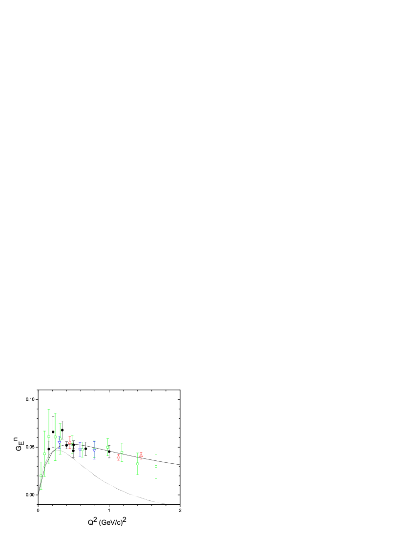
Figure 6: As Fig. 2, but for the neutron electric form factor $G_{E_{n}}$. The experimental data included in the fit are taken from genfit (filled circles). Additional data, not included in the fit, are taken from madey (open triangles) glazier (open inverted triangles) and schiavilla (open squares).

The five remaining coefficients, $\beta_{\rho}$, $\beta_{\omega}$, $\beta_{\varphi}$, $\alpha_{\rho}$, $\alpha_{\varphi}$ and the parameter $\gamma$ are fitted to recent data on electromagnetic form factors. Because of the inconsistencies between different data sets, most notably between those obtained from recoil polarization and Rosenbluth separation, the choice of the data plays an important role in the final outcome. In the present calculation the recoil polarization JLab data for the form factor ratios $R_{p}=\mu_{p}G_{E_{p}}/G_{M_{p}}$ and $R_{n}=\mu_{n}G_{E_{n}}/G_{M_{n}}$ are used in combination with Rosenbluth separation data, mostly from SLAC, for $G_{M_{p}}/\mu_{p}G_{D}$ and $G_{M_{n}}/\mu_{n}G_{D}$, as well as some recent measurements of $G_{E_{n}}$. The data actually used in the fit are quoted in the figure captions to Figs. 2-6 and are indicated by filled symbols. The values of the fitted parameters are: $\beta_{\rho}=0.512$, $\beta_{\omega}=1.129$, $\beta_{\varphi}=-0.263$, $\alpha_{\rho}=2.675$, $\alpha_{\varphi}=-0.200$ and $\gamma=0.515$ (GeV/c)^-2 BI . These values differ somewhat from those obtained in the 1973 fit, although they retain most of their properties, namely a large coupling to the $\omega$ meson in $F_{1}$ and a very large coupling to the $\rho$ meson in $F_{2}$. The spatial extent of the intrinsic structure is somewhat larger than in IJL , $\langle r^{2}\rangle^{1/2}\simeq 0.49$ fm compared to $\simeq 0.34$ fm.

Figs. 2 and 3 show a comparison between the calculation with the parameters given above and the experimental data for the proton magnetic form factor $G_{M_{p}}/\mu_{p}G_{D}$ and the proton form factor ratio $R_{p}$. The results of the 1973 calculation, with no direct coupling to $F_{2}^{V}$, are also shown. One can see that the inclusion of the direct coupling pushes the zero in $R_{p}$ to larger values of $Q^{2}$ (in wan the zero is at $\simeq$ 8 (GeV/c)²). Note that any model parametrized in terms of $F_{1}$ and $F_{2}$ will produce results for $R_{p}$ that are in qualitative agreement with the data, such as a soliton model soliton or relativistic constituent quark models frank ; simula . Perturbation expansions of relativistic effects also produce results that go in the right direction genova .

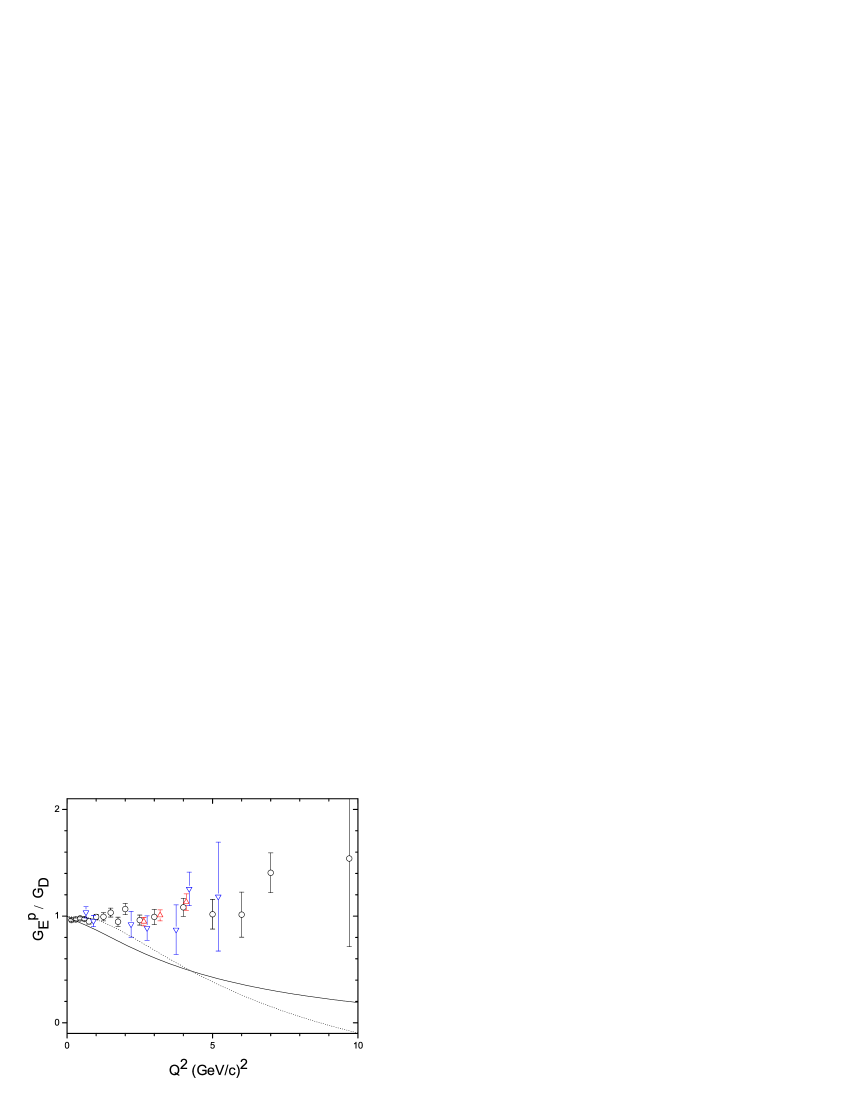
Figure 7: As Fig. 2, but for the proton electric form factor $G_{E_{p}}/G_{D}$. The experimental data, not included in the fit, are obtained from the Rosenbluth separation method walker (open circles), Christy (open inverted triangles) and Qattan (open triangles).

Figs. 4 and 5 show the same comparison, but for the neutron. Contrary to the case of the 1973 parametrization, the present parametrization is in excellent agreement with the neutron data. This is emphasized in Fig. 6 where the electric form factor of the neutron is shown and compared with additional data not included in the fit. However, as one can see from Figs. 2 and 3, the excellent agreement with the neutron data is at the expense of a slight disagreement with proton data. Finally, in Fig. 7 the results for the proton electric form factor is shown in comparison with the experimental data obtained from the Rosenbluth technique. To settle the question of consistency between proton and neutron space-like data, it is very important to extend the existing experimental information to higher values of $Q^{2}$, more specifically:

• Measure the proton form factor ratio $R_{p}$ beyond 6 (GeV/c)² among other things to see whether it indeed goes through zero or not perdrisat .

• Measure the neutron magnetic form factor $G_{M_{n}}$ beyond 2 (GeV/c)². This experiment has been carried out at JLab and is being analyzed at the moment brooks .

• Measure the neutron electric form factor $G_{E_{n}}$ beyond 1.4 (GeV/c)². These experiments will be carried out at JLab Madey and at MIT-Bates Gao .

III.1 Charge and magnetization radii

The low $Q^{2}$ behavior of the electromagnetic form factors provides information about the charge and magnetization radii which are related to the slope of the electric and magnetic form factors in the origin by

$$\left<r^{2}\right>_{E} = -6\,\left.\frac{dG_{E}(Q^{2})}{dQ^{2}}\right|_{Q^{2}=0}~{},$$

$$\left<r^{2}\right>_{M} = -6\,\frac{1}{\mu}\,\left.\frac{dG_{M}(Q^{2})}{dQ^{2}}\right|_{Q^{2}=0}~{}.$$ (16)

In Table 1 the radii from the present calculation are compared to the experimental values. The proton charge radius and the magnetic radii of the proton and the neutron are equal within the error bars. The calculated values show the same behavior. However, the absolute values are underpredicted by a few percent (note that the radii were not included in the fit).

Table 1: Charge and magnetization radii of the nucleon

Radius	Present	Experiment	Reference
$\left<r^{2}\right>^{1/2}_{E_{p}}$	$0.838$	$0.895\pm 0.018$ fm	Sick
		$0.890\pm 0.014$ fm	Udem
		$0.862\pm 0.012$ fm	Simon
$\left<r^{2}\right>^{1/2}_{M_{p}}$	$0.825$	$0.855\pm 0.035$ fm	review
$\left<r^{2}\right>_{E_{n}}$	$-0.100$	$-0.115\pm 0.003$ fm2	Kopecky
$\left<r^{2}\right>^{1/2}_{M_{n}}$	$0.834$	$0.873\pm 0.011$ fm	Kubon

III.2 Scaling laws

Dimensional counting rules count and results from perturbative QCD pqcd show that to leading order the ratio of Pauli and Dirac form factors scales as $F_{2}/F_{1}\propto 1/Q^{2}$. However, the values extracted from the recently obtained data from polarization transfer experiments show that, at least up to $Q^{2}=5.6$ (GeV/c)², this ratio seems to scale rather as $1/Q$. In the VMD approach of IJL this $1/Q$ behavior was shown to be transient, i.e. it is only valid in an intermediate $Q^{2}$ region, but does not hold in the large $Q^{2}$ limit iac1 , whereas in a p-QCD model with nonzero quark orbital angular momenta wave it was argued that the $1/Q$ scaling may be valid to arbitrary large values of $Q^{2}$ ralston . In the latter, it was attributed to the presence of the nonzero orbital angular momentum components in the proton wave function arising from the hadron helicity nonconservation. A similar result was obtained in a relativistic constituent quark model in which the condition of Poincaré invariance induces a violation of hadron helicity conservation miller . On the other hand, in brodsky it was argued that the nonzero orbital angular momentum contributes to both $F_{1}$ and $F_{2}$ in such a way that $F_{2}/F_{1}\propto 1/Q$ for intermediate values of $Q^{2}$ and $\propto 1/Q^{2}$ for large values of the momentum transfer.

In a recent p-QCD analysis of the Pauli form factor the asymptotic behavior of the ratio $F_{2}/F_{1}$ was predicted to be belitsky

$$\frac{F_{2}}{F_{1}}\propto\frac{\ln^{2}(Q^{2}/\Lambda^{2}_{\rm QCD})}{Q^{2}}~{},$$ (17)

indicating that the quantity

$$A\;=\;\frac{Q^{2}}{\ln^{2}(Q^{2}/\Lambda^{2}_{\rm QCD})}\frac{F_{2}}{F_{1}}\;\propto\;1~{},$$ (18)

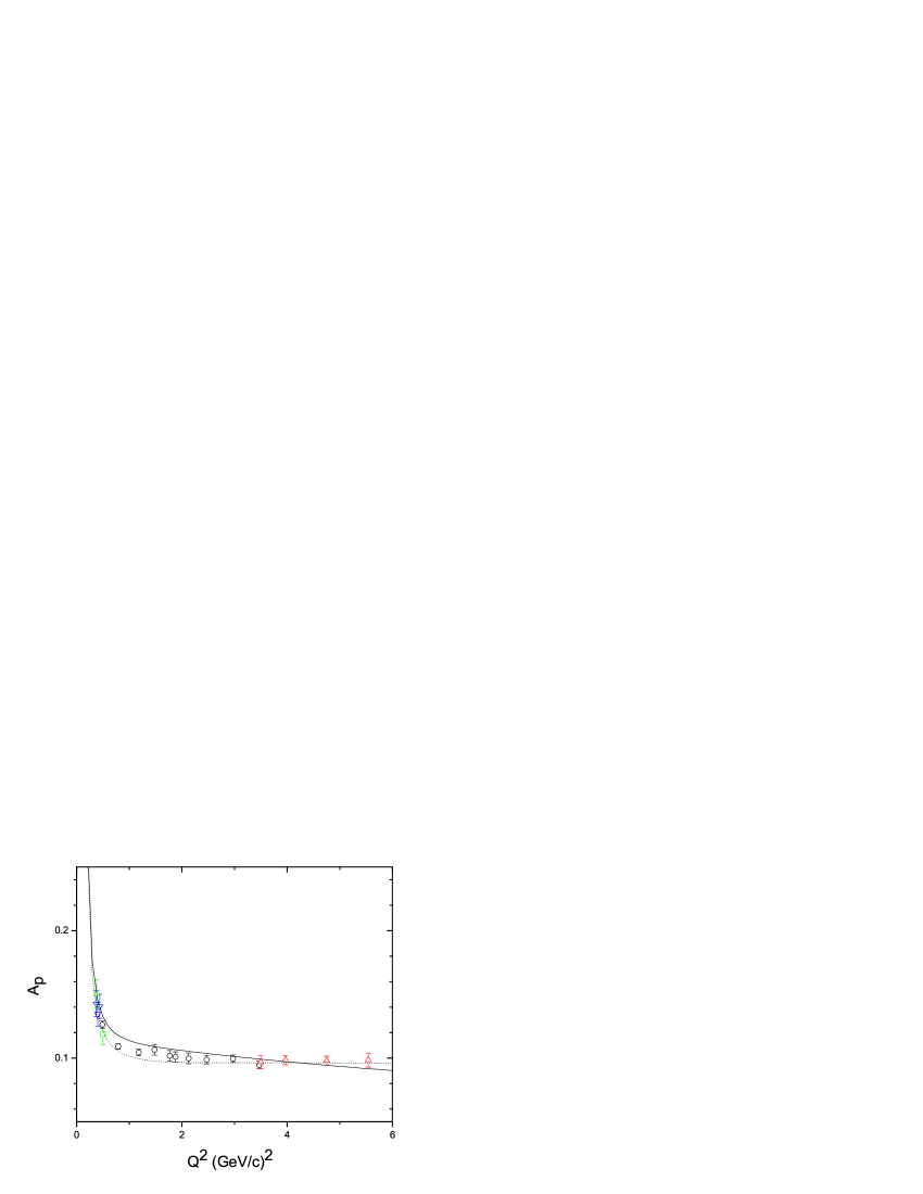
Figure 8: Comparison between the experimental and theoretical values of the ratio $A_{p}=(Q^{2}F_{2,p}/F_{1,p})/\ln^{2}(Q^{2}/\Lambda^{2}_{\rm QCD})$ in the space-like region with $\Lambda_{\rm QCD}=0.300$ GeV/c. The experimental data are taken from jones (open circles), gayou (open triangles), milbrath (open squares) and pospi (open inverted triangles). The solid line is from the present calculation and the dotted line from IJL .

does not depend on $Q^{2}$ in the asymptotic region. The coefficient $\Lambda_{\rm QCD}$ is a soft scale related to the size of the nucleon $\Lambda_{\rm QCD}=0.300$ GeV/c review ; gari . A similar form was obtained in a study of light-front wave functions brodsky . Figs. 8 and 9 show this ratio for the proton and neutron, respectively. The data seem to approach a constant value, even though the domain of validity of p-QCD is expected to set in at much higher values of $Q^{2}$. In order to understand the onset of the perturbative region of QCD, it is crucial to extend the polarization transfer measurements to larger values of $Q^{2}$ both for the proton and the neutron.

IV Time-like form factors

Time-like form factors are important for a global understanding of the structure of the nucleon hammer ; dub ; egle ; BCHH ; TG . In the space-like region ($Q^{2}>0$) the electromagnetic form factors can be studied through electron scattering, whereas in the time-like region ($Q^{2}<0$) they can be measured through the creation or annihilation of a nucleon-antinucleon pair. The time-like structure of the nucleon form factors has recently been analyzed wan in the VMD model of IJL . Here the same approach is used to analyze the time-like structure of the form factors. The method consists in analytically continuing the intrinsic structure to BI

$$g(q^{2})=\frac{1}{(1-\gamma e^{i\theta}q^{2})^{2}}~{},$$ (19)

where $q^{2}=-Q^{2}$ and $\theta$ is a phase. The contribution of the $\rho$ meson is analytically continued for $q^{2}>4m_{\pi}^{2}$ as frazer

$$\frac{m_{\rho}^{2}}{m_{\rho}^{2}-q^{2}}\rightarrow\frac{m_{\rho}^{2}+8\Gamma_{\rho}m_{\pi}/\pi}{m_{\rho}^{2}-q^{2}+(4m_{\pi}^{2}-q^{2})\Gamma_{\rho}[\alpha(q^{2})-i\beta(q^{2})]/m_{\pi}}~{},$$ (20)

where

$$\alpha(q^{2}) = \frac{2}{\pi}\sqrt{\frac{q^{2}-4m_{\pi}^{2}}{q^{2}}}\,\ln\left(\frac{\sqrt{q^{2}-4m_{\pi}^{2}}+\sqrt{q^{2}}}{2m_{\pi}}\right)~{},$$

$$\beta(q^{2}) = \sqrt{\frac{q^{2}-4m_{\pi}^{2}}{q^{2}}}~{}.$$ (21)

The results for the time-like form factors are shown in Figs. 10 and 11. The phase $\theta$ is obtained from a best fit to the proton data: $\theta=0.397$ rad $\simeq 22.7^{\circ}$, compared to the value $\simeq 53^{\circ}$ obtained in wan . It should be noted that the correction to the large $q^{2}$ data discussed in wan has not been done in these figures. One can see from these figures that while the proton form factor, $|G_{M_{p}}|$, obtained from analytic continuation of the present parametrization is in marginal agreement with data, the neutron form factor, $|G_{M_{n}}|$, is in major disagreement. This result points once more to the inconsistency between neutron space-like and time-like data already noted in wan ; hammer . A remeasurement of the neutron time-like data could help to resolve this inconsistency. The result presented here is in contrast with the analysis of wan that was in good agreement with both proton and neutron time-like form factors. In Figs. 12 and 13, the electric form factors $|G_{E_{p}}|$ and $|G_{E_{n}}|$ are shown for future use in the extraction of $|G_{M_{p}}|$ and $|G_{M_{n}}|$ from the data. These figures show that the assumptions $|G_{E_{p}}|=|G_{M_{p}}|$ and $|G_{E_{n}}|=0$ used in the extraction of the magnetic form factors from the experimental data, are not always justified.

V Summary and conclusions

In this contribution, a simultaneous study of the space- and time-like data on the electromagnetic form factors of the nucleon was presented. The analysis was carried out in a two-component model, which consists of an intrinsic (three-quark) structure and a meson cloud whose effects were taken into account via VMD couplings to the $\rho$, $\omega$ and $\varphi$ mesons. The difference with an earlier calculation lies in the treatment of the isovector Pauli form factor $F_{2}^{V}$. The inclusion of an intrinsic component in $F_{2}^{V}$ shows a considerable improvement for the space-like neutron form factors. Since the form factors are related by isospin symmetry, the excellent description description of the neutron form factors is at the expense of a slight disagreement for the proton space-like data. The picture emerging from the present study is that of an intrinsic structure slightly larger in spatial extent than that of wan , $\langle r^{2}\rangle^{1/2}\simeq 0.49$ fm instead of $0.34$ fm, and a contribution of the meson cloud ($q\bar{q}$ pairs) slightly smaller in strength than that of wan , $\alpha_{\rho}=2.675$ instead of $3.706$.

The present calculation is not able to describe the neutron time-like data in a satisfactory way. In effect, a simultaneous description of both the space- and time-like data for the neutron has encountered serious difficulty in the literature hammer ; wan ; BI . It is of the utmost importance to extend the experimental information on the neutron form factors to be able to resolve the observed discrepancies and to obtain a consistent description of all electromagnetic form factors of the nucleon in both the space- and time-like regions.

Recently it was shown BCHH ; TG that the angular dependence of the single-spin and double-spin polarization observables provides a sensitive test of model of nucleon form factors in the time-like region. These polarization observables allow to distinguish between different models of nucleon electromagnetic form factors, even though they fit equally well the nucleon form factors in the space-like region. More work in this direction is in progress.

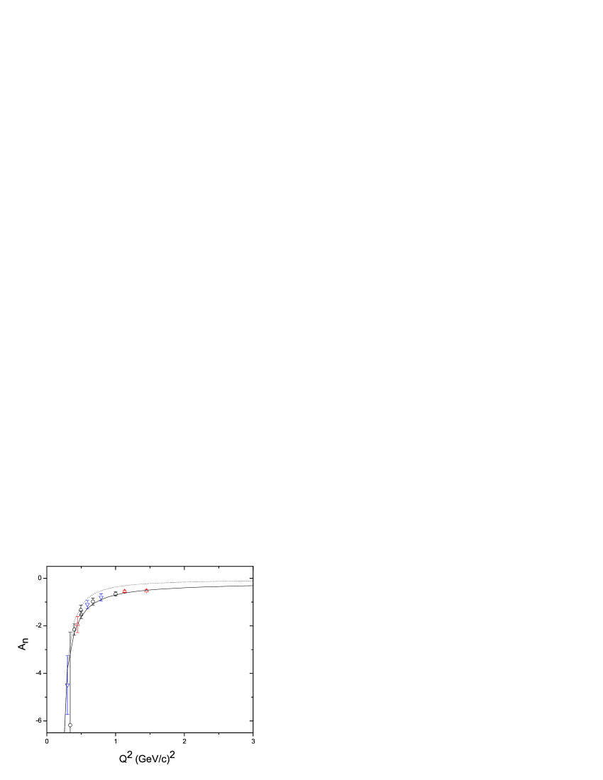
Figure 9: As Fig. 8, but for the neutron. The experimental data are taken from genfit (open circles), madey (open triangles) and glazier (open inverted triangles).

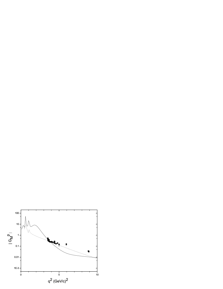
Figure 10: Comparison between experimental and theoretical proton magnetic form factor $|G_{M_{p}}|$ in the time-like region. The experimental values are taken from ptime under the assumption $|G_{E_{p}}|=|G_{M_{p}}|$. The solid lines are from the present analysis and the dotted lines from wan .

Figure 11: As Fig. 10, but for the neutron magnetic form factor $|G_{M_{n}}|$. The experimental values are taken from ntime under the assumption $|G_{E_{n}}|=0$.

Figure 12: As Fig. 10, but for the proton electric form factor $|G_{E_{p}}|$.

Figure 13: As Fig. 10, but for the neutron electric form factor $|G_{E_{n}}|$.

References

- (1) I. Estermann, R. Frisch and O. Stern, Nature 132, 169 (1933).
- (2) R. Hofstadter, Annu. Rev. Nucl. Sci. 7, 231 (1957).
- (3) J.I. Friedman and H.W. Kendall, Annu. Rev. Nucl. Sci. 22, 203 (1972).
-
(4)
M.K. Jones et al.,
Phys. Rev. Lett. 84, 1398 (2000);
V. Punjabi et al., nucl-ex/0501018. -
(5)
O. Gayou et al.,
Phys. Rev. C 64, 038202 (2001);
O. Gayou et al., Phys. Rev. Lett. 88, 092301 (2002). - (6) R.C. Walker et al., Phys. Rev. D 49, 5671 (1994).
- (7) L. Andivahis et al., Phys. Rev. D 50, 5491 (1994).
-
(8)
P.A.M. Guichon and M. Vanderhaeghen,
Phys. Rev. Lett. 91, 142303 (2003);
P.G. Blunden, W. Melnitchouk and J.A. Tjon, Phys. Rev. Lett. 91, 142304 (2003);
Y.-C. Chen, A. Afanasev, S.J. Brodsky, C.E. Carlson and M. Vanderhaeghen, Phys. Rev. Lett. 93, 122301 (2004);
P.G. Blunden, W. Melnitchouk and J.A. Tjon, arXiv:nucl-th/0506039. - (9) M.P. Rekalo and E. Tomasi-Gustafsson, Nucl. Phys. A 740, 271 (2004); Nucl. Phys. A 742, 322 (2004); Eur. Phys. J. A 22, 331 (2004).
- (10) F. Iachello, A.D. Jackson and A. Lande, Phys. Lett. B 43, 191 (1973).
- (11) G. Holzwarth, Z. Phys. A 356, 339 (1996).
- (12) R. Madey et al., Phys. Rev. Lett. 91, 122002 (2003).
- (13) R. Bijker and F. Iachello, Phys. Rev. C 69, 068201 (2004).
- (14) M.N. Rosenbluth, Phys. Rev. 79, 615 (1950).
- (15) P. Bosted et al., Phys. Rev. C 51, 409 (1995).
- (16) S. Galster, H. Klein, J. Moritz, K.H. Schmidt and D. Wegener, Nucl. Phys. B 32, 221 (1971).
- (17) C.E. Hyde-Wright and K. de Jager, Annu. Rev. Nucl. Part. Sci. 54, 217 (2004) (updated version, arXiv:nucl-ex/0507001).
- (18) J. Arrington, Phys. Rev. C 68, 034325 (2003).
- (19) M.E. Christy et al., Phys. Rev. C 70, 015206 (2004).
- (20) I.A. Qattan et al., nucl-ex/0410010.
- (21) J. Arrington et al., arXiv:nucl-ex/0408020.
- (22) G. Höhler et al., Nucl. Phys. B 114, 505 (1976).
- (23) M.F. Gari and W. Krümpelmann, Phys. Lett. B 141, 295 (1984); Z. Phys. A 322, 689 (1985); Phys. Lett. B 173, 10 (1986).
- (24) E.L. Lomon, Phys. Rev. C 64, 035204 (2001).
- (25) M.R. Frank, B.K. Jennings and G.A. Miller, Phys. Rev. C 54, 920 (1996).
- (26) E. Pace, G. Salmè, F. Cardarelli and S. Simula, Nucl. Phys. A 666, 33c (2000).
-
(27)
S.J. Brodsky and G.R. Farrar,
Phys. Rev. Lett. 31, 1153 (1973);
Phys. Rev. D 11, 1309 (1975);
V.A. Matveev, R.M. Muradian and A.N. Tavkhelidze, Lett. Nuovo Cimento 7, 719 (1973). - (28) G.P. Lepage and S.J. Brodsky, Phys. Rev. Lett. 43, 545 (1979); Phys. Rev. D 22, 2157 (1980).
- (29) A. Akhiezer and M.P. Rekalo, Dokl. Akad. Nauk USSR 180, 1081 (1968); Sov. J. Part. Nucl. 4, 277 (1974).
- (30) A.V. Belitsky, X. Ji, and F. Yuan, Phys. Rev. Lett. 91, 092003 (2003).
- (31) S.J. Brodsky, J.R. Hiller, D.S. Hwang and V.A. Karmanov, Phys. Rev. D 69, 076001 (2004).
- (32) R. Bijker, F. Iachello and A. Leviatan, Ann. Phys. (N.Y.) 236, 69 (1994); Phys. Rev. C 54, 1935 (1996).
- (33) W.R. Frazer and J.R. Fulco, Phys. Rev. 117, 1609 (1960).
- (34) F. Iachello and Q. Wan, Phys. Rev. C 69, 055204 (2004).
- (35) B.D. Milbrath et al., Phys. Rev. Lett. 80, 452 (1998); erratum Phys. Rev. Lett. 82, 2221 (1999).
- (36) Th. Pospischil et al., Eur. Phys. J. A 12, 125 (2001).
- (37) F. Cardarelli and S. Simula, Phys. Rev. C 62, 065201 (2000).
-
(38)
M. De Sanctis, M.M. Giannini, L. Repetto and E. Santopinto,
Phys. Rev. C 62, 025208 (2000);
M. De Sanctis, M.M. Giannini, E. Santopinto and A. Vassallo, Eur. Phys. J. A 19, s01, 81 (2004); Rev. Mex. Fís. 50 S2, 96 (2004). -
(39)
S. Rock et al., Phys. Rev. D 46, 24 (1992);
A. Lung et al., Phys. Rev. Lett. 70, 718 (1993);
W. Xu et al., Phys. Rev. Lett. 85, 2900 (2000);
W. Xu et al., Phys. Rev. C 67, 012201 (2003). - (40) G. Kubon et al., Phys. Lett. B 524, 26 (2002).
- (41) D.I. Glazier et al., arXiv:nucl-ex/0410026.
- (42) C. Perdrisat et al., JLab Experiment E01-109.
-
(43)
W.K. Brooks et al., JLab Experiment E94-017;
W.K. Brooks and J.D. Lachniet, arXiv:nucl-ex/0504028. -
(44)
B. Wojtsekhowski et al., JLab Experiment E02-013;
R. Madey et al., JLab Experiment E04-110. - (45) R. Alarcon et al., MIT-Bates proposal E91-09.
-
(46)
C. Herberg et al., Eur. Phys. J. A 5, 131 (1999)
applies FSI corrections to M. Ostrick et al.,
Phys. Rev. Lett. 83, 276 (1999);
I. Passchier et al., Phys. Rev. Lett. 82, 4988 (1999);
H. Zhu et al., Phys. Rev. Lett. 87, 081801 (2001);
J. Golak et al., Phys. Rev. C 63, 034006 (2001) applies FSI corrections to J. Becker et al., Eur. Phys. J. A 6, 329 (1999);
J. Bermuth et al., Phys. Lett. B 564, 199 (2003) updates D. Rohe et al., Phys. Rev. Lett. 83, 4257 (1999);
G. Warren et al., Phys. Rev. Lett. 92, 042301 (2004). - (47) R. Schiavilla and I. Sick, Phys. Rev. C 64, 041002 (2001).
- (48) I. Sick, Phys. Lett. B 576, 62 (2003).
- (49) Th. Udem, A. Huber, B. Gross, J. Reichert, M. Prevedelli, M. Weitz and T.W. Hänsch, Phys. Rev. Lett. 79, 2646 (1997).
- (50) G.G. Simon, Ch. Schmitt, F. Borkowski and V.H. Walther, Nucl. Phys. A 333, 381 (1980).
- (51) S. Kopecky, J.A. Harvey, N.W. Hill, M. Krenn, M. Pernicka, P. Riehs and S. Steiner, Phys. Rev. C 56, 2229 (1997).
- (52) F. Iachello, Eur. Phys. J. A 19, s01, 29 (2004).
- (53) J.P. Ralston and P. Jain, Phys. Rev. D 69, 053008 (2004).
- (54) G.A. Miller and M.R. Frank, Phys. Rev. C 65, 065205 (2002).
- (55) H.-W. Hammer, U.-G. Meissner and D. Drechsel, Phys. Lett. B 385, 343 (1996).
- (56) S. Dubnička, A.Z. Dubničková and P. Weisenpacher, J. Phys. G: Nucl. Part. Phys. 29, 405 (2003).
- (57) E. Tomasi-Gustafsson and M.P. Rekalo, Phys. Lett. B 504, 291 (2001).
- (58) S.J. Brodsky, C.E. Carlson, J.R. Hiller and D.S. Hwang, Phys. Rev. D 69, 054022 (2004).
- (59) E. Tomasi-Gustafsson, F. Lacroix, C. Duterte and G.I. Gakh, Eur. Phys. J. A 24, 419 (2005) [arXiv:nucl-th/0503001].
-
(60)
M. Castellano et al.,
Il Nuovo Cimento A 14, 1 (1973);
G. Bassompierre et al., Phys. Lett. B 68, 477 (1977);
D. Bisello et al., Nucl. Phys. B 224, 379 (1983);
T.A. Armstrong et al., Phys. Rev. Lett. 70, 1212 (1993);
G. Bardin et al., Nucl. Phys. B 411, 3 (1994);
A. Antonelli et al., Phys. Lett. B 334, 431 (1994);
M. Ambrogiani et al., Phys. Rev. D 60, 032002 (1999). - (61) A. Antonelli et al., Nucl. Phys. B 517, 3 (1998).