Electromagnetic structure of $A$=2 and 3 nuclei and the nuclear current operator

Abstract

Different models for conserved two- and three-body electromagnetic currents are constructed from two- and three-nucleon interactions, using either meson-exchange mechanisms or minimal substitution in the momentum dependence of these interactions. The connection between these two different schemes is elucidated. A number of low-energy electronuclear observables, including (i) $np$ radiative capture at thermal neutron energies and deuteron photodisintegration at low energies, (ii) $nd$ and $pd$ radiative capture reactions, and (iii) isoscalar and isovector magnetic form factors of ³H and ³He, are calculated in order to make a comparative study of these models for the current operator. The realistic Argonne $v_{18}$ two-nucleon and Urbana IX or Tucson-Melbourne three-nucleon interactions are taken as a case study. For $A$=3 processes, the bound and continuum wave functions, both below and above deuteron breakup threshold, are obtained with the correlated hyperspherical-harmonics method. Three-body currents give small but significant contributions to some of the polarization observables in the ²H($p,\gamma$)³He process and the ²H($n,\gamma$)³H cross section at thermal neutron energies. It is shown that the use of a current which did not exactly satisfy current conservation with the two- and three-nucleon interactions in the Hamiltonian was responsible for some of the discrepancies reported in previous studies between the experimental and theoretical polarization observables in $p$$d$ radiative capture.

I Introduction

The present study investigates a number of different models for the nuclear electromagnetic current derived from realistic interactions. The emphasis is on constructing two- and three-body currents which satisfy the current conservation relation (CCR) with the corresponding two- and three-nucleon interactions. Two different methods are adopted to achieve this goal: one is based on meson-exchange mechanisms, the other uses minimal substitution in the explicit and implicit–through the isospin exchange operator–momentum dependence of the interactions. A by-product of this analysis is, in particular, the elucidation of the sense in which these two different methods are related to each other.

A variety of electromagnetic observables involving the $A$=2 and 3 nuclei are taken as case study for these current operator models, including the $n$$p$ radiative capture at thermal neutron energy, the deuteron photodisintegration at low energy, the magnetic form factors of ³He and ³H, and the $n$$d$ and $p$$d$ radiative captures. These processes have been extensively studied in the past by several research groups (for a review, see Ref. Car98 ). Most recently, the authors of the present paper (and collaborators) have investigated the $A$=3 radiative capture reactions below deuteron breakup threshold in Refs. Viv96 ; Viv00 , and the trinucleon form factors in Ref. Mar98 . Below, we briefly review those aspects of these earlier works that are more pertinent to the present study.

The $A$=3 bound- and scattering-state wave functions were obtained using the pair-correlated hyperspherical harmonics (PHH) method Kie93 ; Kie94 ; Kie01 from a realistic Hamiltonian model consisting of the Argonne $v_{18}$ two-nucleon Wir95 and Urbana IX three-nucleon interaction Pud95 (AV18/UIX). This technique allows for the inclusion of the Coulomb interaction in both the bound and scattering states. The nuclear electromagnetic current operator included, in addition to one-body convection and spin-magnetization terms, two- and three-body terms. The dominant two-body terms were constructed using meson-exchange mechanisms Ris85a from the momentum-independent part of the AV18, including the long-range pion-exchange component, and coincide with those derived here within the same approach. They satisfy the CCR with this part of the interaction.

The two-body currents originating from the spin-orbit components of the AV18 were constructed using again meson-exchange mechanisms Car90 ($\sigma$ and $\omega$ exchanges for the isospin-independent, and $\rho$ exchange for the isospin dependent terms), while those from the quadratic momentum-dependent components were obtained by gauging only the momentum operators Sch89 , but ignoring the implicit momentum dependence which comes through the isospin exchange operator. The resulting currents are not strictly conserved. This lack of current conservation was pointed out in Ref. Sch89 , but has not been sufficiently emphasized in subsequent papers, mostly because of the short-range character of these currents and their generally small associated contributions to photo- and electronuclear processes, for example see Refs. Viv96 ; Car90 ; Sch89 ; Sch91 . The overcome of this limitation is one of the main aims of this work.

Earlier studies, as well as the present one, also take into account the two-body currents, associated with the $\rho\pi\gamma$ and $\omega\pi\gamma$ transition mechanisms and with the excitation of intermediate $\Delta$ resonances (for a review, see again Ref. Car98 ). However, these currents are purely transverse, and therefore unconstrained by the CCR. They are not the focus of the present work.

The effects of $\Delta$-isobar degrees of freedom in nuclear electroweak processes were studied more thoroughly in Refs. Mar98 ; Sch92 , using two different approximations. One was based on first-order perturbation theory (referred to above), while the other retained explicit one- and two-$\Delta$ admixtures in the nuclear wave functions via the transition-correlation-operator (TCO) method Sch92 . This latter approach is inherently non-perturbative. In particular, it generates three-body currents Mar98 , which are strictly not consistent with the three-nucleon interaction in the Hamiltonian. In the present work these currents will be derived directly from the three-nucleon interaction, and will satisfy by construction the CCR with it.

The derived new models for the electromagnetic current are tested in this paper on a variety of $A$=2 and 3 processes. The predictions for the $np$ radiative capture and deuteron electrodisintegration cross sections at low energies remain practically unchanged and are in agreement with the experimental data. For $A$=3 the situation is more interesting since the two-body currents play a very important role. For example, in Refs. Viv96 ; Viv00 it was found that two-body currents play a crucial role in reproducing the cross section and polarization observables measured in $p$$d$ and $n$$d$ radiative captures. However, some significant discrepancies remained unresolved. In the $n$$d$ case, the theoretical prediction for the total cross section at thermal energies exceeds the experimental value by 14%. With the present model of the current, the overprediction is reduced to 9%. The origin of this overestimate is still puzzling, particularly in view of the fact that the astrophysical $S$-factor for the $p$$d$ radiative capture at zero energy is calculated to be within 1% Mar04 of that extrapolated from cross section measurements in the range $\simeq 2\div 20$ keV Lun02 .

In the $p$$d$ case, the calculated tensor observables $T_{20}$ and $T_{21}$ at center-of-mass (c.m.) energy of 2 MeV Viv00 were found to be at variance with data. In that same work, it was also shown that these observables are sensitive to the small (suppressed) contributions arising from electric dipole transitions between the initial $p$$d$ $P$-wave scattering states with spin channel $S=3/2$ and the final ³He bound state. When these contributions were calculated in the long-wavelength-approximation (LWA) using the Siegert form of the $E_{1}$ operator, the resulting tensor observables were much closer to the experimental values. Since the year 2000, more accurate PHH wave functions have become available for the $A$=3 nuclei, and the calculations for $pd$ radiative capture could be extended at energies above deuteron breakup threshold Viv03 ; Mar03a ; Mar03b . In preliminary calculations Viv03 , we found that also at 3.33 MeV the theory could not reproduce the precise data for the tensor polarization observables $T_{20}$ and $T_{21}$ Goe92 . In the present work, it will be shown how the use of a conserved current indeed removes the discrepancy between theory and experiment for these observables. Furthermore, the calculation has been extended up to 20 MeV.

In Ref. Mar98 it was shown that the theoretical predictions for the magnetic form factors of ³He and ³H were in satisfactory agreement with experimental data at low and moderate values of the momentum transfer. The first diffraction region, however, was poorly reproduced by the theoretical calculation, especially in the ³He case. The three-body current operators, constructed within the TCO approach, gave only very small contributions. This discrepancy is not resolved in the present study.

Alternative descriptions of the $A$=2 and 3 electromagnetic processes have been also recently reported. A conserved current model was developed by Arenohövel and collaborators Buc85 and applied to $A$=2 reactions Aren00 ; Aren04 . Several groups are studying electromagnetic processes in the three-nucleon system. In Refs. Golak00 ; Skib03 , the nucleons are taken as interacting via two- and three-nucleon potentials. The electromagnetic currents are then constructed using the meson exchange scheme for satisfying the CCR, but only with a part of the interaction. In Ref. Schad01 , the meson exchange currents are taken into account using the Siegert’s theorem Sieg37 . No three-body currents are considered in these works. In Ref. Delt04 , a nuclear model is employed which allows for the excitation of a nucleon to a $\Delta$ isobar, and the two-body forces and currents are generated by the exchange of mesons. The $\Delta$ excitation yields also effective three-body forces and three-body currents. However, this current model does not satisfy exactly the CCR with the adopted Hamiltonian as discussed in Ref. Delt04 . Very recently, models of the currents derived from chiral Lagrangians are starting to appear BS04 . In all these calculations, the Coulomb interaction between protons in the scattering state is disregarded. Note that, in spite of the differences of the various approaches, the theoretical predictions of Refs. Skib03 ; Schad01 ; Delt04 and of this paper turn out to be, for most of the observables, quantitatively quite similar. An example will be presented for $nd$ radiative capture, where the theoretical results are free from the uncertainty related to the omission of the Coulomb interaction. Also other approaches, as the Lorentz integral transform technique ELOT00 , have been applied to study the electromagnetic response of the trinucleon systems.

This paper is organized into six sections and three appendices. In Sec. II and III we discuss the model for the two- and three-body current operators, respectively. In Sec. IV, we briefly review the PHH method for the $pd$ and $nd$ scattering-state wave function, below and above deuteron breakup threshold. In Sec. V we present results for the magnetic structure of the $A$=3 nuclei, for the deuteron photodisintegration cross section at low energy, for the $np$ radiative capture at thermal neutron energies, and for $nd$ and $pd$ radiative captures at c.m. energies up to 20 MeV. Finally, in Sec. VI, we summarize our conclusions. The connection between the meson-exchange and minimal-substitution approaches is elaborated in Appendix A, while a collection of formulas for the two-body current operators associated with the quadratic momentum-dependent terms of the two-nucleon interaction, and for the three-body current operators in configuration space, are given in the Appendices B and C.

II Two-body current

The nuclear electromagnetic charge, $\rho({\bm{q}})$, and current, ${\bm{j}}({\bm{q}})$, operators can be written as sums of one-, two-, and many-body terms that operate on the nucleon degrees of freedom:

$$\rho({\bm{q}}) = \sum_{i}\rho_{i}({\bm{q}})+\sum_{i<j}\rho_{ij}({\bm{q}})+\ldots\ ,$$ (1)

$${\bm{j}}({\bm{q}}) = \sum_{i}{\bm{j}}_{i}({\bm{q}})+\sum_{i<j}{\bm{j}}_{ij}({\bm{q}})+\ldots\ .$$ (2)

The one-body operators $\rho_{i}({\bm{q}})$ and ${\bm{j}}_{i}({\bm{q}})$ are derived from the non-relativistic reduction of the covariant single-nucleon current, by expanding in powers of $1/m$, $m$ being the nucleon mass. In the notation of Ref. Car98 , the one-body charge operator in configuration space is given by

$$\rho_{i}({\bm{q}})=\rho_{i,{\rm NR}}({\bm{q}})+\rho_{i,{\rm RC}}({\bm{q}})\ ,$$ (3)

where the leading order term, labeled NR, is

$$\rho_{i,{\rm NR}}({\bm{q}})=\epsilon_{i}{\rm e}^{{\rm i}{\bm{q}}\cdot{\bm{r}}_{i}}\ ,$$ (4)

with

$$\epsilon_{i}=\frac{1}{2}\left[G_{E}^{S}(q_{\mu}^{2})+G_{E}^{V}(q_{\mu}^{2})\tau_{i,z}\right]\ ,$$ (5)

while the term labeled RC is proportional to $1/m^{2}$ and is explicitly listed in Ref. Car98 . In Eq. (5) $G_{E}^{S}(q_{\mu}^{2})$ and $G_{E}^{V}(q_{\mu}^{2})$ are the isoscalar and isovector combinations of the nucleon electric Sachs form factors, respectively, evaluated at the four-momentum transfer $q_{\mu}^{2}$.

The electromagnetic current operator must satisfy the current conservation relation (CCR)

$${\bm{q}}\cdot{\bm{j}}({\bm{q}})=[H,\rho({\bm{q}})]\ ,$$ (6)

where the nuclear Hamiltonian $H$ is taken to consist, quite generally, of two- and three-body interactions, denoted as $v_{ij}$ and $V_{ijk}$ respectively,

$$H=\sum_{i}{{\bm{p}}_{i}^{2}\over 2m}+\sum_{i<j}v_{ij}+\sum_{i<j<k}V_{ijk}\ .$$ (7)

Realistic models for these interactions contain isospin- and momentum-dependent terms which do not commute with the charge operators. To lowest order in $1/m$, Eq. (6) separates into

$${\bm{q}}\cdot{\bm{j}}_{i}({\bm{q}}) = \biggl{[}{{\bm{p}}_{i}^{2}\over 2m},\rho_{i,{\rm NR}}({\bm{q}})\biggr{]}\ ,$$ (8)

$${\bm{q}}\cdot{\bm{j}}_{ij}({\bm{q}}) = [v_{ij},\rho_{i,{\rm NR}}({\bm{q}})+\rho_{j,{\rm NR}}({\bm{q}})]\ ,$$ (9)

and similarly for the three-body current ${\bm{j}}_{ijk}({\bm{q}})$. It has been tacitly assumed that two-body terms in $\rho({\bm{q}})$ are of order $1/m^{2}$. The one-body current is easily shown to satisfy Eq. (8). However, it is rather difficult to construct conserved two- and three-body currents.

It is useful to adopt the classification scheme of Ref. Ris89 , and separate the current ${\bm{j}}_{ij}({\bm{q}})$ into model-independent (MI) and model-dependent (MD) parts,

$${\bm{j}}_{ij}({\bm{q}})={\bm{j}}_{ij}^{MI}({\bm{q}})+{\bm{j}}_{ij}^{MD}({\bm{q}})\ .$$ (10)

The MI two-body current ${\bm{j}}_{ij}^{MI}({\bm{q}})$ has a longitudinal component, constructed so as to satisfy the CCR of Eq. (9) (see following subsections), while the MD two-body current ${\bm{j}}_{ij}^{MD}({\bm{q}})$ is purely transverse and therefore is un-constrained by the CCR. The latter will not be discussed any further in the present section; it suffices to say that it is taken to consist of the isoscalar $\rho\pi\gamma$ and isovector $\omega\pi\gamma$ transition currents, as well as of the isovector current associated with excitation of intermediate $\Delta$ resonances Viv96 ; Viv00 ; Mar98 .

A method to derive ${\bm{j}}_{ij}^{MI}({\bm{q}})$ was developed by Riska and collaborators Ris85a ; Sch89 ; Ris85b ; Ris85c and Arenhövel and collaborators Buc85 (see Ref. Car98 for a review). An alternative approach, which we will revisit and generalize in the present work, is based on ideas first proposed by Sachs in Ref. Sac48 , and later applied by Nyman in Ref. Nym67 to derive the magnetic-dipole transition operator due to the one-pion-exchange potential. We will refer to these two different approaches as the “meson-exchange” (ME) and “minimal-substitution” (MS) scheme, respectively. To appreciate the differences and similarities between them, they are discussed in the two following subsections.

In the rest of the paper, we will use the following notation: a generic nucleon-nucleon interaction will be written as

$$v_{ij}=v^{IC}_{ij}+v^{IB}_{ij}\ ,\qquad v^{IC}_{ij}=v^{0}_{ij}+v^{p}_{ij}\ ,$$ (11)

where $v^{IC}_{ij}$ and $v^{IB}_{ij}$ are the isospin-symmetry conserving ($I$$C$) and breaking ($I$$B$) parts of the potential, respectively. In turn, $v^{0}_{ij}$ and $v^{p}_{ij}$ are the momentum-independent and momentum-dependent components of $v^{IC}_{ij}$, respectively. The next two subsections deal with the $v^{IC}_{ij}$ part of the potential. The two-body current associated with its $v^{IB}_{ij}$ part will be considered in Sec. II.3.

For later reference in Sec. V, a summary of the models for two-body current operators used in the present work is given in Sec. II.4.

II.1 The two-body current operator in the meson-exchange scheme

First consider the isospin-conserving momentum-independent part of the potential $v^{0}_{ij}$, which can be written as

$$v^{0}_{ij}=v_{1,ij}+v_{2,ij}\,{\bm{\tau}}_{i}\cdot{\bm{\tau}}_{j}\ ,$$ (12)

where ${\bm{\tau}}_{i}$ and ${\bm{\tau}}_{j}$ are the isospin Pauli matrices, and $v_{1}$ and $v_{2}$ are in general functions of the positions and spin operators of the two nucleons; $v_{2}$ includes the long-range one-pion-exchange component. In particular, the isospin-dependent terms are given by

$$v_{2,ij}\,{\bm{\tau}}_{i}\cdot{\bm{\tau}}_{j}=[v_{\tau}(r_{ij})+v_{\sigma\tau}(r_{ij})\,{\bm{\sigma}}_{i}\cdot{\bm{\sigma}}_{j}+v_{t\tau}(r_{ij})\,S_{ij}]\,{\bm{\tau}}_{i}\cdot{\bm{\tau}}_{j}\ ,$$ (13)

where $S_{ij}$ is the standard tensor operator, ${\bm{\sigma}}_{i}$ and ${\bm{\sigma}}_{j}$ are the spin Pauli matrices, and the notation of Ref. Wir84 is used. In momentum-space, $v_{2}$ reads

$$v_{2}({\bm{k}})\,{\bm{\tau}}_{i}\cdot{\bm{\tau}}_{j}=[v_{\tau}(k)+v_{\sigma\tau}(k)\,k^{2}\,{\bm{\sigma}}_{i}\cdot{\bm{\sigma}}_{j}+v_{t\tau}(k)S_{ij}({\bm{k}})]{\bm{\tau}}_{i}\cdot{\bm{\tau}}_{j}\ ,$$ (14)

where $v_{\tau}(k)$, $v_{\sigma\tau}(k)$ and $v_{t\tau}(k)$ are related to their configuration-space counter-parts by the relations

$$v_{\tau}(k) = 4\pi\int_{0}^{\infty}r^{2}dr\,j_{0}(kr)v_{\tau}(r)\>\>,$$ (15)

$$v_{\sigma\tau}(k) = \frac{4\pi}{k^{2}}\int_{0}^{\infty}r^{2}dr\,\left[j_{0}(kr)-1\right]v_{\sigma\tau}(r)\>\>,$$ (16)

$$v_{t\tau}(k) = \frac{4\pi}{k^{2}}\int_{0}^{\infty}r^{2}dr\,j_{2}(kr)v_{t\tau}(r)\>\>.$$ (17)

The factor $[j_{0}(kr)-1]$ in the expression for $v_{\sigma\tau}(k)$ ensures that the volume integral of $v_{\sigma\tau}(r)$ vanishes Sch89 , and the tensor operator in momentum-space is defined as $S_{ij}({\bm{k}})=k^{2}({\bm{\sigma}}_{i}\cdot{\bm{\sigma}}_{j})-3({\bm{\sigma}}_{i}\cdot{\bm{k}})({\bm{\sigma}}_{j}\cdot{\bm{k}})$.

If the isospin-dependent interaction $v_{2}({\bm{k}})$ is assumed to be induced by $\pi$- and $\rho$-meson exchanges, as for example in the Bonn model Mac01 , then

$$v_{2}({\bm{k}})\,{\bm{\tau}}_{i}\cdot{\bm{\tau}}_{j}=\Big{[}v_{\rho S}(k)+[2v_{\rho}(k)+v_{\pi}(k)]\,k^{2}\,{\bm{\sigma}}_{i}\cdot{\bm{\sigma}}_{j}+[v_{\rho}(k)-v_{\pi}(k)]S_{ij}({\bm{k}})\Big{]}\,{\bm{\tau}}_{i}\cdot{\bm{\tau}}_{j}\ ,$$ (18)

with

$$v_{\pi}(k) = -{\frac{f_{\pi NN}^{2}}{3m_{\pi}^{2}}}{\frac{f^{2}_{\pi}(k)}{k^{2}+m_{\pi}^{2}}}\ ,$$ (19)

$$v_{\rho}(k) = -{\frac{g_{\rho NN}^{2}(1+\kappa_{\rho NN})^{2}}{12m^{2}}}{\frac{f^{2}_{\rho}(k)}{k^{2}+m_{\rho}^{2}}}\ ,$$ (20)

$$v_{\rho S} = g_{\rho NN}^{2}\frac{f^{2}_{\rho}(k)}{k^{2}+m_{\rho}^{2}}\ ,$$ (21)

where $f_{\pi NN}$, and $g_{\rho NN}$ and $\kappa_{\rho NN}$ are the coupling constants of the $\pi$- and $\rho$-mesons, $f_{\pi}(k)$ and $f_{\rho}(k)$ are the associated form factors (usually, of monopole type), $m_{\pi}$ and $m_{\rho}$ are their masses, and finally $m$ is the nucleon mass.

More generally, if one assumes that the interaction $v_{2}({\bm{k}})$ is due to the exchange of a number of “$\pi$-like” pseudoscalar ($PS$) and “$\rho$-like” vector ($V$) mesons, then one finds

$$v_{2}({\bm{k}})\,{\bm{\tau}}_{i}\cdot{\bm{\tau}}_{j}=\Big{[}v_{VS}(k)+[2v_{V}(k)+v_{PS}(k)]\,k^{2}\,{\bm{\sigma}}_{i}\cdot{\bm{\sigma}}_{j}+[v_{V}(k)-v_{PS}(k)]S_{ij}({\bm{k}})\Big{]}\,{\bm{\tau}}_{i}\cdot{\bm{\tau}}_{j}\ ,$$ (22)

where the functions $v_{PS}(k)$, $v_{V}(k)$, and $v_{VS}(k)$ are given by

$$v_{PS}(k) = \sum_{a=1}^{N}f^{2}_{PS,a}\frac{1}{k^{2}+m_{a}^{2}}\>\>\>,$$ (23)

$$v_{V}(k) = \sum_{a=1}^{N}f^{2}_{V,a}\frac{1}{k^{2}+m_{a}^{2}}\>\>\>,$$ (24)

$$v_{VS}(k) = \sum_{a=1}^{N}f^{2}_{VS,a}\frac{1}{k^{2}+m_{a}^{2}}\>\>\>.$$ (25)

In the expressions above, $m_{a}$ is the mass and $f^{2}_{PS,a}\equiv-f^{2}_{\pi NN,a}/3m^{2}_{a}$, $f^{2}_{V,a}\equiv-g_{\rho NN,a}^{2}(1+\kappa_{\rho NN,a})^{2}/12m^{2}$ and $f^{2}_{VS,a}\equiv g_{\rho NN,a}^{2}$ are the coupling constants of the exchanged $a$-meson. These parameters are fixed so that

$$v_{PS}(k) = [v_{\sigma\tau}(k)-2\>v_{t\tau}(k)]/3\>\>\>,$$ (26)

$$v_{V}(k) = [v_{\sigma\tau}(k)+v_{t\tau}(k)]/3\>\>\>,$$ (27)

$$v_{VS}(k) = v_{\tau}(k)\>\>\>,$$ (28)

where $v_{\sigma\tau}(k)$, $v_{t\tau}(k)$, and $v_{\tau}(k)$ are given in Eqs. (15)–(17).

The two-body currents due to these $PS$- and $V$-meson exchanges are then derived by minimal substitution in the effective $PS$-$NN$ and $V$-$NN$ coupling Lagrangians. The non-relativistic reduction of the associated Feynman amplitudes in momentum space leads to:

$${\bm{j}}_{ij}({\bm{k}}_{i},{\bm{k}}_{j};PS) = 3{\rm i}\,G_{E}^{V}(q_{\mu}^{2})({\bm{\tau}}_{i}\times{\bm{\tau}}_{j})_{z}\bigg{[}v_{PS}(k_{j}){\bm{\sigma}}_{i}({\bm{\sigma}}_{j}\cdot{\bm{k}}_{j})-v_{PS}(k_{i}){\bm{\sigma}}_{j}({\bm{\sigma}}_{i}\cdot{\bm{k}}_{i})$$ (29)

$$+{{\bm{k}}_{i}-{\bm{k}}_{j}\over k_{i}^{2}-k_{j}^{2}}\bigl{[}v_{PS}(k_{i})-v_{PS}(k_{j})\bigr{]}({\bm{\sigma}}_{i}\cdot{\bm{k}}_{i})({\bm{\sigma}}_{j}\cdot{\bm{k}}_{j})\bigg{]}\ ,$$

$${\bm{j}}_{ij}({\bm{k}}_{i},{\bm{k}}_{j};V) = -3{\rm i}\,G_{E}^{V}(q_{\mu}^{2})({\bm{\tau}}_{i}\times{\bm{\tau}}_{j})_{z}\bigg{[}v_{V}(k_{j}){\bm{\sigma}}_{i}\times({\bm{\sigma}}_{j}\times{\bm{k}}_{j})-v_{V}(k_{i}){\bm{\sigma}}_{j}\times({\bm{\sigma}}_{i}\times{\bm{k}}_{i})$$ (30)

$$-{v_{V}(k_{i})-v_{V}(k_{j})\over k_{i}^{2}-k_{j}^{2}}\bigl{[}({\bm{k}}_{i}-{\bm{k}}_{j})({\bm{\sigma}}_{i}\times{\bm{k}}_{i})\cdot({\bm{\sigma}}_{j}\times{\bm{k}}_{j})$$

$$+({\bm{\sigma}}_{i}\times{\bm{k}}_{i})\>{\bm{\sigma}}_{j}\cdot({\bm{k}}_{i}\times{\bm{k}}_{j})+({\bm{\sigma}}_{j}\times{\bm{k}}_{j})\>{\bm{\sigma}}_{i}\cdot({\bm{k}}_{i}\times{\bm{k}}_{j})\bigr{]}\bigg{]}\ ,$$

$${\bm{j}}_{ij}({\bm{k}}_{i},{\bm{k}}_{j};VS) = -{\rm i}\,G_{E}^{V}(q_{\mu}^{2})({\bm{\tau}}_{i}\times{\bm{\tau}}_{j})_{z}\,{{\bm{k}}_{i}-{\bm{k}}_{j}\over k_{i}^{2}-k_{j}^{2}}\,[v_{VS}(k_{i})-v_{VS}(k_{j})]\ ,$$ (31)

where ${\bm{k}}_{i}$ and ${\bm{k}}_{j}$ are the fractional momenta delivered to nucleon $i$ and $j$, with ${\bm{k}}_{i}+{\bm{k}}_{j}={\bm{q}}$, and $G_{E}^{V}(q_{\mu}^{2})$ is the isovector combination of the nucleon electric Sachs form factors Car98 . The current

$${\bm{j}}^{ME}_{ij}({\bm{k}}_{i},{\bm{k}}_{j};v^{0})={\bm{j}}_{ij}({\bm{k}}_{i},{\bm{k}}_{j};PS)+{\bm{j}}_{ij}({\bm{k}}_{i},{\bm{k}}_{j};V)+{\bm{j}}_{ij}({\bm{k}}_{i},{\bm{k}}_{j};VS)\ ,$$ (32)

satisfies exactly the CCR with the potential given in Eq. (12).

Configuration-space expressions are obtained from

$${\bm{j}}_{ij}({\bm{q}};B)=\int d{{\bm{x}}}\>{\rm e}^{{\rm i}{\bm{q}}\cdot{{\bm{x}}}}\int\frac{d{\bm{k}}_{i}}{(2\pi)^{3}}\frac{d{\bm{k}}_{j}}{(2\pi)^{3}}{\rm e}^{{\rm i}{\bm{k}}_{i}\cdot({\bm{r}}_{i}-{{\bm{x}}})}{\rm e}^{{\rm i}{\bm{k}}_{j}\cdot({\bm{r}}_{j}-{{\bm{x}}})}{\bm{j}}_{ij}({\bm{k}}_{i},{\bm{k}}_{j};B)\ ,$$ (33)

where $B$=$PS$, $V$ or $VS$, and can be found in the Appendix of Ref. Sch89 . For later reference, we report below the configuration-space expression for the current associated with the isospin-dependent central potential ${\bm{j}}_{ij}({\bm{q}};VS)$:

$${\bm{j}}_{ij}({\bm{q}};VS) = -G_{E}^{V}(q_{\mu}^{2})\,({\bm{\tau}}_{i}\times{\bm{\tau}}_{j})_{z}\,{\rm e}^{{\rm i}{\bm{q}}\cdot{\bm{R}}}\,\sum_{a=1}^{N}\frac{f^{2}_{VS,a}}{4\pi}\int_{-1/2}^{1/2}\,dx\,\biggl{(}{{\rm i}x{\bm{q}}\over L_{a}(x)}+\hat{\bm{r}}\biggr{)}{\rm e}^{-{\rm i}x{\bm{q}}\cdot{\bm{r}}}\,{\rm e}^{-rL_{a}(x)}\ ,$$

$$L_{a}(x) = \sqrt{m_{a}^{2}+\frac{q^{2}}{4}\Big{(}1-4x^{2}\Big{)}}\ ,$$ (34)

where ${\bm{r}}\equiv{{\bm{r}}}_{i}-{{\bm{r}}}_{j}$ and ${\bm{R}}\equiv({\bm{r}}_{i}+{\bm{r}}_{j})/2$.

The construction of the two-body currents associated with the isospin-conserving momentum-dependent part of the interaction $v^{p}_{ij}$ is less straightforward. A procedure similar to the one just reviewed has been applied to the case of the currents from the spin-orbit components of the interaction Car90 . It consists, in essence, of attributing these to exchanges of “$\sigma$-like” and “$\omega$-like” mesons for the isospin-independent terms, and to “$\rho$-like” mesons for the isospin-dependent ones. Explicit expressions for the resulting currents can be found in Ref. Car90 .

The two-body currents from the quadratic momentum-dependent terms of the interaction are listed in Ref. Sch89 and were obtained by minimal substitution, that is ${{\bm{p}}}_{i}\rightarrow{{\bm{p}}}_{i}-\epsilon_{i}\,{\bm{A}}({\bm{r}}_{i})$. While minimal substitution ensures current conservation for the isospin-independent (quadratic-momentum-dependent) components of the interaction, this prescription does not lead to a conserved current for the isospin-dependent ones. Indeed, the commutator in Eq. (9) gives rise to an isovector term proportional to $({\bm{\tau}}_{i}\times{\bm{\tau}}_{j})_{z}$, which cannot be generated by minimal substitution (for a discussion of this point, see Ref. Sch04 ). These isovector currents were ignored in all previous work since, in view of their short range, they were expected to give negligible contributions.

The currents associated with $v^{IB}_{ij}$, which have never been considered up until now, will be discussed in Sec. II.3.

II.2 The two-body current operator in the minimal-substitution scheme

Consider again the isospin-conserving momentum-independent part of the potential given in Eqs. (12) and (13). The isospin operator ${\bm{\tau}}_{i}\cdot{\bm{\tau}}_{j}$ is formally equivalent to an implicit momentum dependence Sac48 , since it can be expressed in terms of the space-exchange operator, $P_{ij}$, using the formula

$${\bm{\tau}}_{i}\cdot{\bm{\tau}}_{j}=-1-(1+{\bm{\sigma}}_{i}\cdot{\bm{\sigma}}_{j})P_{ij}\ ,$$ (35)

valid when operating on antisymmetric wave functions, as in the case of a fermionic system. The space-exchange operator is defined as

$$P_{ij}\,f({\bm{r}}_{i},{\bm{r}}_{j})\equiv{\rm e}^{{\bm{r}}_{ji}\cdot{{\bm{\nabla}}}_{i}+{\bm{r}}_{ij}\cdot{{\bm{\nabla}}}_{j}}\,f({\bm{r}}_{i},{\bm{r}}_{j})=f({\bm{r}}_{j},{\bm{r}}_{i})\ ,$$ (36)

where the ${{\bm{\nabla}}}$-operators act only on the generic function $f({\bm{r}}_{i},{\bm{r}}_{j})$ and not on the vectors ${\bm{r}}_{ij}={\bm{r}}_{i}-{\bm{r}}_{j}=-{\bm{r}}_{ji}$ in the exponential. In the presence of an electromagnetic field, after performing minimal substitution, the operator $P_{ij}$ becomes Sac48

$$P_{ij}\rightarrow{P}^{\bm{A}}_{ij} = {\rm e}^{{\bm{r}}_{ji}\cdot[{{\bm{\nabla}}}_{i}-{\rm i}\epsilon_{i}{\bm{A}}({\bm{r}}_{i})]+{\bm{r}}_{ij}\cdot[{{\bm{\nabla}}}_{j}-{\rm i}\epsilon_{j}{\bm{A}}({\bm{r}}_{j})]}$$ (37)

$$\equiv {\rm e}^{{\bm{r}}_{ji}\cdot{{\bm{\nabla}}}_{i}+g_{i}({\bm{r}}_{i})}\,{\rm e}^{{\bm{r}}_{ij}\cdot{{\bm{\nabla}}}_{j}+g_{j}({\bm{r}}_{j})}\ ,$$

where ${\bm{A}}({\bm{r}})$ is the vector potential, and the functions $g_{i}({\bm{r}}_{i})$ and $g_{j}({\bm{r}}_{j})$ have been defined as $g_{i}({\bm{r}}_{i})\equiv-{\rm i}\,\epsilon_{i}\,{\bm{r}}_{ji}\cdot{\bm{A}}({\bm{r}}_{i})$ and $g_{j}({\bm{r}}_{j})\equiv-{\rm i}\,\epsilon_{j}\,{\bm{r}}_{ij}\cdot{\bm{A}}({\bm{r}}_{j})$. The operator ${P}^{\bm{A}}_{ij}$ is then the product of two operators, each having the general form

$$P({\bm{r}})={\rm e}^{{\bf a}\cdot{{\bm{\nabla}}}+g({\bm{r}})}\ ,$$ (38)

where ${\bf a}$ is a vector independent of ${\bm{r}}$. It has been shown in Ref. Sac48 that $P({\bm{r}})$ can expressed as

$$P({\bm{r}})={\rm e}^{{1\over a}\int_{\bm{r}}^{{\bm{r}}+{\bf a}}ds\,g({\bm{s}})}\,{\rm e}^{{\bf a}\cdot{{\bm{\nabla}}}}\ ,$$ (39)

where $ds$ is an infinitesimal element of a straight line parallel to ${\bf a}$, which goes from position ${\bm{r}}$ to position ${\bm{r}}+{\bf a}$. Using this general result in Eq. (37), we obtain

$${P}^{\bm{A}}_{ij}={\rm e}^{-{\rm i}\epsilon_{i}\int_{{\bm{r}}_{i}}^{{\bm{r}}_{j}}d{\bm{s}}\cdot{\bm{A}}({\bm{s}})-{\rm i}\epsilon_{j}\int_{{\bm{r}}_{j}}^{{\bm{r}}_{i}}d{\bm{s}}^{\prime}\cdot{\bm{A}}({\bm{s}}^{\prime})}P_{ij}\ ,$$ (40)

with $d{\bm{s}}=ds\,{\hat{\bm{r}}}_{ji}$ and $d{\bm{s}}^{\prime}=ds\,{\hat{\bm{r}}}_{ij}$. The line integrals are performed on straight lines parallel to ${\hat{\bm{r}}_{ji}}$ and ${\hat{\bm{r}}_{ij}}$.

The procedure of Ref. Sac48 leading to Eq. (40) can be generalized and the two integrals can be performed on two generic paths $\gamma_{ij}$ and $\gamma^{\prime}_{ji}$, that go from position $i$ to position $j$ and vice versa, as shown in Fig. 1. Indeed, for a gauge transformation

$${\bm{A}}({\bm{r}}) \rightarrow {\bm{A}}({\bm{r}})-{\bm{\nabla}}G({\bm{r}})\ ,$$ (41)

$$\Psi \rightarrow {\rm e}^{{\rm i}\sum_{i}\epsilon_{i}G({\bm{r}}_{i})}\;\Psi\ ,$$ (42)

where $G({\bm{r}})$ is a generic function, it can be shown that the state

$${\bm{\tau}}_{i}\cdot{\bm{\tau}}_{j}\Psi=\bigg{[}-1-(1+{\bm{\sigma}}_{i}\cdot{\bm{\sigma}}_{j})P^{\bm{A}}_{ij}\bigg{]}\;\Psi\ ,$$ (43)

where $P^{\bm{A}}_{ij}$ is given in Eq. (40) with the generic integration paths of Fig. 1, transforms as

$$\bigg{[}-1-(1+{\bm{\sigma}}_{i}\cdot{\bm{\sigma}}_{j})P^{\bm{A}}_{ij}\bigg{]}\;\Psi \rightarrow \bigg{[}-1-(1+{\bm{\sigma}}_{i}\cdot{\bm{\sigma}}_{j})P^{{\bm{A}}-{\bm{\nabla}}G}_{ij}\bigg{]}\;{\rm e}^{{\rm i}\sum_{i}\epsilon_{i}G({\bm{r}}_{i})}\;\Psi$$ (44)

$$= {\rm e}^{{\rm i}\sum_{i}\epsilon_{i}G({\bm{r}}_{i})}\;\bigg{[}-1-(1+{\bm{\sigma}}_{i}\cdot{\bm{\sigma}}_{j})P^{\bm{A}}_{ij}\bigg{]}\;\Psi\ ,$$

in conformity with the requirements of gauge invariance of the theory. A conserved current can then be derived by considering an infinitesimal gauge transformation, as discussed in Ref. Sac48 .

Rather than following the general procedure of Ref. Sac48 , we obtain the current in the limit of weak electromagnetic fields, since calculations of photo- and electronuclear observables are typically carried out in first-order perturbation theory in these fields. Then, by retaining only linear terms in the vector potential, we find

$$v_{ij} \rightarrow v_{1,ij}+v_{2,ij}\bigg{[}-1-(1+{\bm{\sigma}}_{i}\cdot{\bm{\sigma}}_{j}){P}^{\bm{A}}_{ij}\bigg{]}$$ (45)

$$\simeq v^{0}_{ij}+v_{2,ij}\,\bigg{[}-{\rm i}\epsilon_{i}\int_{\gamma_{ij}}d{\bm{s}}\cdot{\bm{A}}({\bm{s}})-{\rm i}\epsilon_{j}\int_{\gamma^{\prime}_{ji}}d{\bm{s}}^{\prime}\cdot{\bm{A}}({\bm{s}}^{\prime})\bigg{]}(1+{\bm{\tau}}_{i}\cdot{\bm{\tau}}_{j})$$

$$\equiv v^{0}_{ij}-\int{\bm{j}}_{ij}({{\bm{x}}})\cdot{\bm{A}}({{\bm{x}}})d{{\bm{x}}}\ ,$$

where the paths $\gamma_{ij}$ and $\gamma^{\prime}_{ji}$ are those illustrated in Fig. 1, and in the second and third lines of the equation above $v^{0}_{ij}$ is as defined in Eq. (12). The current density operator is then given by

$${\bm{j}}_{ij}({{\bm{x}}})={\rm i}\,v_{2,ij}\,\bigg{[}\epsilon_{i}\int_{\gamma_{ij}}d{\bm{s}}\,\delta({{\bm{x}}}-{\bm{s}})+\epsilon_{j}\int_{\gamma^{\prime}_{ji}}d{\bm{s}}^{\prime}\,\delta({{\bm{x}}}-{\bm{s}}^{\prime})\bigg{]}\,(1+{\bm{\tau}}_{i}\cdot{\bm{\tau}}_{j})\ ,$$ (46)

and its Fourier transform reads

$${\bm{j}}_{ij}({\bm{q}})={\rm i}\,v_{2,ij}\bigg{(}\epsilon_{i}\int_{\gamma_{ij}}d{\bm{s}}\,{\rm e}^{{\rm i}{\bm{q}}\cdot{\bm{s}}}+\epsilon_{j}\int_{\gamma^{\prime}_{ji}}d{\bm{s}}^{\prime}\,{\rm e}^{{\rm i}{\bm{q}}\cdot{\bm{s}}^{\prime}}\bigg{)}\,(1+{\bm{\tau}}_{i}\cdot{\bm{\tau}}_{j})\ .$$ (47)

A number of comments are now in order. Firstly, the current in Eq. (47) by construction satisfies the CCR

$${\bm{q}}\cdot{\bm{j}}_{ij}({\bm{q}})=\biggl{[}v^{0}_{ij},\rho_{i,{\rm NR}}({\bm{q}})+\rho_{j,{\rm NR}}({\bm{q}})\biggr{]}\ .$$ (48)

This is easily verified by observing that along any path from ${\bm{r}}_{i}$ to ${\bm{r}}_{j}$

$${\rm i}{\bm{q}}\cdot\int_{{\bm{r}}_{i}}^{{\bm{r}}_{j}}\!d{\bm{s}}\;{\rm e}^{{\rm i}{\bm{q}}\cdot{\bm{s}}}={\rm e}^{{\rm i}{\bm{q}}\cdot{\bm{r}}_{j}}-{\rm e}^{{\rm i}{\bm{q}}\cdot{\bm{r}}_{i}}\ ,$$ (49)

and that

$${\rm i}\,(\epsilon_{i}-\epsilon_{j})(1+{\bm{\tau}}_{i}\cdot{\bm{\tau}}_{j})=G_{E}^{V}(q_{\mu}^{2})\,({\bm{\tau}}_{i}\times{\bm{\tau}}_{j})_{z}\ .$$ (50)

Secondly, because of the arbitrariness of the two integration paths, the prescription just outlined does not lead to a unique two-body current. Moreover, if $v_{2,ij}$ consists of a sum of different terms, then, for each of these, different paths $\gamma_{ij}$ and $\gamma^{\prime}_{ji}$ can be selected. Hence, Eq. (47) can be interpreted as a parameterization of all possible two-body currents which satisfy the CCR with the two-body potential given in Eq. (12). In particular, it is interesting to note that the longitudinal part of the two-body currents of Eqs. (29)–(34) obtained in the ME approach can also be derived in the MS scheme. This connection is shown in Appendix A.

Thirdly, the choice of a linear path ($LP$) for $\gamma_{ij}$ and $\gamma^{\prime}_{ji}$ in Eq. (47) (as in Ref. Sac48 ), namely

$${\bm{s}}=-{\bm{s}}^{\prime}={\bm{r}}_{i}-x{\bm{r}}_{ij}\ ,\hskip 28.45274pt0\leq x\leq 1\ ,\\$$ (51)

gives

$${\bm{j}}^{LP}_{ij}({\bm{q}})={\rm i}\,v_{2,ij}\,G_{E}^{V}(q_{\mu}^{2})\,({\bm{\tau}}_{i}\times{\bm{\tau}}_{j})_{z}\,{\bm{r}}_{ij}\,f_{ij}({\bm{q}})\ ,$$ (52)

with

$$f_{ij}({\bm{q}})\equiv\frac{{\rm e}^{{\rm i}{\bm{q}}\cdot{\bm{r}}_{i}}-{\rm e}^{{\rm i}{\bm{q}}\cdot{\bm{r}}_{j}}}{{\bm{q}}\cdot{\bm{r}}_{ij}}\ .$$ (53)

Note that $f_{ij}({\bm{q}}=0)={\rm i}$.

Lastly, it is important to observe that, in the limit $q\rightarrow 0$, the current operator ${\bm{j}}_{ij}({\bm{q}})$ becomes path-independent, i.e. it is unique, and is given by

$${\bm{j}}_{ij}({\bm{q}}=0)=-v_{2,ij}G_{E}^{V}(q_{\mu}^{2})\,({\bm{\tau}}_{i}\times{\bm{\tau}}_{j})_{z}\,{\bm{r}}_{ij}\ .$$ (54)

This result can also be derived in a more direct way by considering the following identities

$${\bm{j}}_{ij}({\bm{q}}=0)=\int d{\bm{x}}\,{\bm{j}}_{ij}({\bm{x}}) = -\int d{\bm{x}}\,{\bm{x}}\,{\bm{\nabla}}\cdot{\bm{j}}_{ij}({\bm{x}})$$ (55)

$$= {\rm i}\,\left[v_{2,ij}\,,\,\int d{\bm{x}}\,{\bm{x}}\left[\rho_{i,{\rm NR}}({\bm{x}})+\rho_{j,{\rm NR}}({\bm{x}})\right]\right]\ ,$$

where in the first line the volume integral of ${\bm{j}}_{ij}({\bm{x}})$ has been re-expressed in terms of the divergence of the current, ignoring vanishing surface contributions, and in the second line use has been made of the CCR. Evaluation of the commutator leads to Eq. (54) above. Note that, mutatis mutandis, namely ${\bm{j}}_{ij}({\bm{x}})\rightarrow{\bm{j}}({\bm{x}})$ and $v_{2,ij}\rightarrow H$, etc., the second line of Eq. (55) is, in essence, the Siegert theorem for the electric dipole operator, to which ${\bm{j}}({\bm{q}}=0)$ is proportional.

We now derive the current operators associated with the momentum-dependent operators of the two-nucleon interaction, within the present scheme. In the case of the spin-orbit interactions, $v^{p}_{1}$ and $v^{p}_{2}$ of Eq. (12) are

$$v^{p}_{1,ij} = v_{b}(r)\,{\bm{L}}\cdot{\bm{S}}\ ,$$

$$v^{p}_{2,ij} = v_{b\tau}(r)\,{\bm{L}}\cdot{\bm{S}}\ ,$$ (56)

where the notation of Refs. Wir95 ; Wir84 is used, and ${\bm{L}}={\bm{r}}_{ij}\times({{\bm{p}}}_{i}-{{\bm{p}}}_{j})/2$, ${{\bm{p}}}_{i}$ and ${{\bm{p}}}_{j}$ being the particles’ momentum operators. Performing minimal substitution in $v_{1}$, we obtain

$${\bm{j}}_{ij}({\bm{q}};b)=\frac{1}{2}v_{b}(r)\biggl{(}\epsilon_{i}\,{\rm e}^{{\rm i}{\bm{q}}\cdot{\bm{r}}_{i}}-\epsilon_{j}\,{\rm e}^{{\rm i}{\bm{q}}\cdot{\bm{r}}_{j}}\biggr{)}\,{\bm{S}}\times{\bm{r}}_{ij}\ .$$ (57)

For the isospin-dependent term $v^{p}_{2}$, we first symmetrize as

$$v^{p}_{2,ij}\,{\bm{\tau}}_{i}\cdot{\bm{\tau}}_{j}=\frac{1}{2}v_{b\tau}(r)\left({\bm{L}}\cdot{\bm{S}}\,{\bm{\tau}}_{i}\cdot{\bm{\tau}}_{j}+{\bm{\tau}}_{i}\cdot{\bm{\tau}}_{j}\,{\bm{L}}\cdot{\bm{S}}\right)\ ,$$ (58)

and then perform minimal substitution in both ${\bm{L}}\cdot{\bm{S}}$ and ${\bm{\tau}}_{i}\cdot{\bm{\tau}}_{j}$. When only terms linear in the vector potential ${\bm{A}}$ are kept and the path $\gamma_{ji}^{\prime}=-\gamma_{ij}$ is taken, the associated current is found to be

$${\bm{j}}_{ij}({\bm{q}};b\tau) = \frac{1}{4}v_{b\tau}(r){\bm{S}}\times{\bm{r}}_{ij}\,\biggl{(}\eta_{j}{\rm e}^{{\rm i}{\bm{q}}\cdot{\bm{r}}_{i}}-\eta_{i}{\rm e}^{{\rm i}{\bm{q}}\cdot{\bm{r}}_{j}}\biggr{)}$$ (59)

$$+ \frac{1}{2}v_{b\tau}(r)G_{E}^{V}(q_{\mu}^{2})({\bm{\tau}}_{i}\times{\bm{\tau}}_{j})_{z}\biggl{(}\,{\bm{L}}\cdot{\bm{S}}\,\int_{\gamma_{ij}}d{\bm{s}}\,{\rm e}^{{\rm i}{\bm{q}}\cdot{\bm{s}}}+\int_{\gamma_{ij}}d{\bm{s}}\,{\rm e}^{{\rm i}{\bm{q}}\cdot{\bm{s}}}\,\,{\bm{L}}\cdot{\bm{S}}\,\biggr{)}\ ,$$

with $\eta_{i}=G_{E}^{S}(q_{\mu}^{2})\,{\bm{\tau}}_{i}\cdot{\bm{\tau}}_{j}+G_{E}^{V}(q_{\mu}^{2})\tau_{i,z}$. In particular, the linear path of Eq. (51) leads to

$${\bm{j}}_{ij}^{LP}({\bm{q}};b\tau) = \frac{1}{4}v_{b\tau}(r){\bm{S}}\times{\bm{r}}_{ij}\,\biggl{(}\eta_{j}{\rm e}^{{\rm i}{\bm{q}}\cdot{\bm{r}}_{i}}-\eta_{i}{\rm e}^{{\rm i}{\bm{q}}\cdot{\bm{r}}_{j}}\biggr{)}$$ (60)

$$+ \frac{\rm i}{2}v_{b\tau}(r)G_{E}^{V}(q_{\mu}^{2})({\bm{\tau}}_{i}\times{\bm{\tau}}_{j})_{z}\biggl{[}\,{\bm{L}}\cdot{\bm{S}}\,\,{\bm{r}}_{ij}\,f_{ij}({\bm{q}})+{\bm{r}}_{ij}\,f_{ij}({\bm{q}})\,{\bm{L}}\cdot{\bm{S}}\,\biggr{]}\ ,$$

with $f_{ij}({\bm{q}})$ defined in Eq. (53).

The current operators associated with the quadratic momentum-dependent terms of the interaction can be derived in a similar fashion. Their explicit expressions are listed in Appendix B.

II.3 Two-body current associated with the isospin-symmetry breaking interactions

The current operators constructed so far in the ME and MS schemes satisfy the CCR with the isospin symmetric component of the two-nucleon potential. However, the latest realistic models of the nucleon-nucleon interaction contain isospin-symmetry breaking terms. In the notation of Ref. Wir95 , this part is written as

$$v^{IB}_{ij}=\sum_{p=15}^{18}v_{p}(r_{ij})O^{p}_{ij}\ ,$$ (61)

and the four isospin-symmetry breaking operators have the form:

$$O^{p=15,\ldots,18}_{ij}=T_{ij}\>\>\>,\,{\bm{\sigma}}_{i}\cdot{\bm{\sigma}}_{j}T_{ij}\>\>\>,\,S_{ij}\,T_{ij}\>\>\>,\,(\tau_{i,z}+\tau_{j,z})\ ,$$ (62)

where $S_{ij}$ is the standard tensor operator and the isotensor operator $T_{ij}$ is defined as $T_{ij}=3\tau_{i,z}\,\tau_{j,z}-{\bm{\tau}}_{i}\cdot{\bm{\tau}}_{j}$. The dependence on ${\bm{\tau}}_{i}\cdot{\bm{\tau}}_{j}$ generates two-body currents which can be taken into account by modifying the isospin-dependent central, spin-spin and tensor terms of the potential as

$${\hat{v}_{\tau}}(r) = [\,v_{\tau}(r)-v_{15}(r)\,]\ ,$$

$${\hat{v}_{\sigma\tau}}(r) = [\,v_{\sigma\tau}(r)-v_{16}(r)\,]\ ,$$

$${\hat{v}_{t\tau}}(r) = [\,v_{t\tau}(r)-v_{17}(r)\,]\ ,$$ (63)

and by using ${\hat{v}_{\tau}}(r)$, ${\hat{v}_{\sigma\tau}}(r)$, and ${\hat{v}_{t\tau}}(r)$, instead of $v_{\tau}(r)$, $v_{\sigma\tau}(r)$, and $v_{t\tau}(r)$ in $v_{2,ij}$ of Eq. (13). However, the contributions associated with the currents from these isospin-symmetry breaking terms have been found to be negligibly small for all the observables of interest here.

II.4 Summary of two-body current models

For the sake of clarity and for later reference, we summarize here the salient features of the three different models for the model-independent current ${\bm{j}}_{ij}^{MI}({\bm{q}})$ corresponding to the AV18 interaction Wir95 , considered in the present paper.

• Old-ME model. This model is that introduced in Refs. Viv96 ; Viv00 ; Mar98 and discussed in Sec. II.1. It is given by

  $${\bm{j}}^{MI,{\rm old}}_{ij}({\bm{q}})={\bm{j}}_{ij}^{ME}({\bm{q}};v^{0})+{\bm{j}}_{ij}^{ME}({\bm{q}};v^{p})\ .$$ (64)

  We re-emphasize that, while ${\bm{j}}_{ij}^{ME}({\bm{q}};v^{0})$ satisfies the CCR with $v^{0}_{ij}$ (which includes the long-range one-pion-exchange term), ${\bm{j}}_{ij}^{ME}({\bm{q}};v^{p})$ is not strictly conserved, as discussed in Sec. II.1.

• New-ME model. This model retains ${\bm{j}}_{ij}^{ME}({\bm{q}};v^{0})$ for the momentum-independent interaction, as in the “old-ME” model. For the momentum-dependent interaction, it uses instead the two-body current obtained in the MS scheme with a linear path, explicitly

  $${\bm{j}}^{MI,{\rm new}}_{ij}({\bm{q}})={\bm{j}}_{ij}^{ME}({\bm{q}};v^{0})+{\bm{j}}_{ij}^{LP}({\bm{q}};v^{p})\ ,$$ (65)

  where

  $${\bm{j}}_{ij}^{LP}({\bm{q}};v^{p})={\bm{j}}_{ij}({\bm{q}};b)+{\bm{j}}_{ij}^{LP}({\bm{q}};b\tau) + {\bm{j}}_{ij}({\bm{q}};LL)+{\bm{j}}_{ij}^{LP}({\bm{q}};LL\tau)$$ (66)

  $$+ {\bm{j}}_{ij}({\bm{q}};bb)+{\bm{j}}_{ij}^{LP}({\bm{q}};bb\tau)\ ,$$

  and ${\bm{j}}_{ij}({\bm{q}};b)$, ${\bm{j}}_{ij}^{LP}({\bm{q}};b\tau)$, ${\bm{j}}_{ij}({\bm{q}};LL)$, ${\bm{j}}_{ij}^{LP}({\bm{q}};LL\tau)$, ${\bm{j}}_{ij}({\bm{q}};bb)$ and ${\bm{j}}_{ij}^{LP}({\bm{q}};bb\tau)$ are listed respectively in Eqs. (57), (60), (127), (128), (132), (133). In addition, the isospin-symmetry-breaking contributions are included via Eq. (63). The two-body current operator given above satisfies exactly the CCR with the AV18 potential.

  It is important to stress that the longitudinal component of ${\bm{j}}_{ij}^{ME}({\bm{q}};v^{0})$ can also be obtained in the MS scheme, as discussed in the previous section and in Appendix A.

• Linear path MS ($LP$-MS) model. This model uses a two-body current obtained in the MS scheme using a linear path, explicitly

  $${\bm{j}}^{MI,LP}_{ij}({\bm{q}})={\bm{j}}_{ij}^{LP}({\bm{q}};v^{0})+{\bm{j}}_{ij}^{LP}({\bm{q}};v^{p})\ ,$$ (67)

  where ${\bm{j}}_{ij}^{LP}({\bm{q}};v^{0})$ is the current given in Eq. (52) and ${\bm{j}}_{ij}^{LP}({\bm{q}};v^{p})$ is the same as in Eq. (66).

III Three-body Current

Three-body currents involving the excitation of an intermediate $\Delta$ resonance were derived recently in the context of a study of explicit $\Delta$ components in the trinucleon wave functions Mar98 ; Delt04 . In addition, the three-body current associated with $S$-wave $\pi$$N$ scattering on an intermediate nucleon was also included in Ref. Mar98 . The conclusion of that work was that these three-body mechanisms give a small contribution to the magnetic form factors of ³H and ³He over a wide range of momentum transfer. However, the three-body currents considered in Ref. Mar98 were not strictly consistent with the three-nucleon interaction (TNI) included in the Hamiltonian.

In this section we generalize the meson-exchange (ME) and minimal substitution (MS) approaches to the case of the three-body current induced by a TNI $V_{ijk}$. The resulting current satisfies, by construction, the CCR with $V_{ijk}$. To be specific, we consider below the Urbana-IX model Pud95 , but the methods that are developed are applicable to other phenomenological models of TNI’s, such as the Tucson-Melbourne Coo79 and Brazil Rob ones.

III.1 The three-body current in the meson-exchange scheme

The Urbana-type TNI is written as sum of a short-range spin- and isospin-independent term and a term involving the excitation of an intermediate $\Delta$ resonance. The central term is irrelevant to the following discussion and is therefore ignored, while the $\Delta$-excitation term is given by Pud95

$$V_{ijk} = \sum_{{\rm cyclic}\,ijk}V_{j;ki}\ ,$$ (68)

$$V_{j;ki} = A_{2\pi}\bigg{(}\{X_{ij}\,,\,X_{jk}\}\,\{{\bm{\tau}}_{i}\cdot{\bm{\tau}}_{j}\,,\,{\bm{\tau}}_{j}\cdot{\bm{\tau}}_{k}\}\,+\frac{1}{4}\,[X_{ij}\,,\,X_{jk}]\,[{\bm{\tau}}_{i}\cdot{\bm{\tau}}_{j}\,,\,{\bm{\tau}}_{j}\cdot{\bm{\tau}}_{k}]\ \bigg{)}\ ,$$ (69)

where $\{\ldots\}$ ($[\ldots]$) denotes the anticommutator (commutator),

$$X_{ij}=v_{\sigma\tau}^{II}(r){\bm{\sigma}}_{i}\cdot{\bm{\sigma}}_{j}+v_{t\tau}^{II}(r)S_{ij}\ ,\\$$ (70)

and $v_{\sigma\tau}^{II}(r)$ and $v_{t\tau}^{II}(r)$ are the standard spin-isospin and tensor-isospin functions occurring in the one-pion-exchange interaction, modified by a short-range gaussian cutoff. The parameter $A_{2\pi}$ as well as the strength of the central term are determined by reproducing the triton binding energy in a Green’s function Monte Carlo calculation, and the nuclear matter equilibrium density in an approximate hypernetted-chain variational calculation Pud95 .

In momentum space, $V_{j;ki}$ can be conveniently expressed as

$$V_{j;ki}({\bm{k}}_{j},{\bm{k}}_{i},{\bm{k}}_{k})=\frac{9}{2}\,A_{2\pi}\,\biggl{[}v_{jk}^{\dagger}({\bm{k}}_{k};\Delta N\rightarrow NN)\,v_{ij}({\bm{k}}_{i};NN\rightarrow N\Delta)\,+{\rm h.\,c.}\biggr{]}\delta({\bm{k}}_{i}+{\bm{k}}_{j}+{\bm{k}}_{k})\ ,$$ (71)

where the $N\Delta$-transition interaction is defined as

$$v_{ij}({\bm{k}};NN\rightarrow N\Delta)=\biggl{[}v_{\sigma\tau}^{II}(k)\,k^{2}\,{\bm{\sigma}}_{i}\cdot{\bf S}_{j}+v_{t\tau}^{II}(k)S_{ij}^{II}({\bm{k}})\biggr{]}\,{\bm{\tau}}_{i}\cdot{\bf T}_{j}\ .$$ (72)

Here ${\bf S}_{j}$ and ${\bf T}_{j}$ are the spin- and isospin-transition operators that convert nucleon $j$ into a $\Delta$-isobar, and $S_{ij}^{II}({\bm{k}})$ is the momentum-space tensor operator in which the Pauli spin operator of particle $j$ is replaced by ${\bf S}_{j}$. The functions $v_{\sigma\tau}^{II}(k)$ and $v_{t\tau}^{II}(k)$ are related to their configuration-space counter-parts by similar relations to those in Eqs. (16) and (17). The momentum transfers to nucleons $i$, $j$, $k$, respectively ${\bm{k}}_{i}$, ${\bm{k}}_{j}$, and ${\bm{k}}_{k}$, sum up to zero. Manipulation of products of transition spin and/or isospin operators is facilitated by making use of the following identity:

$${\bf S}_{\alpha}^{\dagger}\,\,{\bf S}_{\beta}=\frac{2}{3}\delta_{\alpha\,\beta}\,-\,\frac{\rm i}{3}\epsilon_{\alpha\,\beta\,\gamma}{\bm{\sigma}}_{\gamma}\ .$$ (73)

The $N\Delta$-transition interaction is assumed to originate from exchanges of “$\pi$-like” ($PS$) and “$\rho$-like” ($V$) mesons, with the associated components $v_{PS}^{II}(k)$ and $v_{V}^{II}(k)$ related to $v_{\sigma\tau}^{II}(k)$ and $v_{t\tau}^{II}(k)$ by relations identical to those in Eqs. (26) and (27). Thus, the $PS$- and $V$-exchange three-body currents, illustrated in Fig. 2, in momentum space read

$${\bm{j}}^{ME}_{j;ki}({\bm{q}}) = \frac{9}{2}\,A_{2\pi}\,\biggl{[}v_{jk}^{\dagger}({\bm{k}}_{k};\Delta N\rightarrow NN)\,\bigl{[}{\bm{j}}_{ij}^{II}({\bm{k}}_{i},{\bm{k}}_{j};PS)\,+{\bm{j}}_{ij}^{II}({\bm{k}}_{i},{\bm{k}}_{j};V)\bigr{]}$$ (74)

$$+ \bigl{[}{\bm{j}}_{jk}^{II}({\bm{k}}_{j},{\bm{k}}_{k};PS)\,+{\bm{j}}_{jk}^{II}({\bm{k}}_{j},{\bm{k}}_{k};V)\bigr{]}^{\dagger}v_{ij}({\bm{k}}_{i};NN\rightarrow N\Delta)+{\rm h.\,c.}\biggr{]}\ ,$$

where the $PS$ and $V$ currents ${\bm{j}}_{ij}^{II}({\bm{k}}_{i},{\bm{k}}_{j};PS)$ and ${\bm{j}}_{ij}^{II}({\bm{k}}_{i},{\bm{k}}_{j};V)$ involving $\Delta$ excitation are obtained from Eqs. (29) and (30) with the replacements ${\bm{\sigma}}_{j}\,({\bm{\tau}}_{j})\rightarrow{\bf S}_{j}\,({\bf T}_{j})$. Configuration-space expressions are listed in Appendix C. Finally, the current above satisfies the CCR with the TNI of Eq. (71).

III.2 The three-body current in the minimal-substitution scheme

Consider the isospin dependence of the TNI. The anticommutator term is first expressed as

$$\{{\bm{\tau}}_{i}\cdot{\bm{\tau}}_{j}\,,\,{\bm{\tau}}_{j}\cdot{\bm{\tau}}_{k}\}=2\,{\bm{\tau}}_{i}\cdot{\bm{\tau}}_{k}\ ,$$ (75)

and the associated current ${\bm{j}}^{A}_{j;ki}({\bm{q}})$ is then derived with the same methods discussed in Sec. II.2 and is given by (see Eq. (47))

$${\bm{j}}^{A}_{j;ki}({\bm{q}})=2{\rm i}\,A_{2\pi}\,\{X_{ij}\,,\,X_{jk}\}\biggl{(}\epsilon_{i}\int_{\gamma_{ik}}d{\bm{s}}\,{\rm e}^{{\rm i}{\bm{q}}\cdot{\bm{s}}}+\epsilon_{k}\int_{\gamma_{ki}^{\prime}}d{\bm{s}}^{\prime}\,{\rm e}^{{\rm i}{\bm{q}}\cdot{\bm{s}}^{\prime}}\biggr{)}\,(1+{\bm{\tau}}_{i}\cdot{\bm{\tau}}_{k})\ ,$$ (76)

where $\gamma_{ik}$ and $\gamma_{ki}^{\prime}$ are generic paths from ${\bm{r}}_{i}$ to ${\bm{r}}_{k}$ and ${\bm{r}}_{k}$ to ${\bm{r}}_{i}$ (see Fig. 3).

In the case of the commutator term, we first note that

$$\frac{1}{4}[{\bm{\tau}}_{i}\cdot{\bm{\tau}}_{j}\,,\,{\bm{\tau}}_{j}\cdot{\bm{\tau}}_{k}]=P_{ij}^{\tau}P_{jk}^{\tau}-P_{jk}^{\tau}P_{ij}^{\tau}\ ,$$ (77)

where $P_{ij}^{\tau}$=$(1+{\bm{\tau}}_{i}\cdot{\bm{\tau}}_{j})/2$ is the isospin-exchange operator. The product $P_{ij}^{\tau}P_{jk}^{\tau}$, when acting on antisymmetric wave functions, is equivalent to

$$P_{ij}^{\tau}P_{jk}^{\tau}=P_{jk}^{\sigma}P_{ij}^{\sigma}P_{jk}P_{ij}\ ,$$ (78)

where $P_{ij}^{\sigma}$ is the spin-exchange operator, defined similarly as $P_{ij}^{\tau}$, and $P_{ij}$ is space-exchange operator introduced in Eq. (36). Note the ordering of the operators on the r.h.s. of the equation above. Obviously, the product $P_{jk}^{\tau}P_{ij}^{\tau}$ is given by a relation similar to Eq. (78) in which the order of the $jk$ and $ij$ pairs is inverted. The products of space exchange operators $P_{jk}P_{ij}$ and $P_{ij}P_{jk}$ are equivalent, respectively, to the exchanges $({\bm{r}}_{i},{\bm{r}}_{j},{\bm{r}}_{k})\rightarrow({\bm{r}}_{k},{\bm{r}}_{i},{\bm{r}}_{j})$ and $({\bm{r}}_{i},{\bm{r}}_{j},{\bm{r}}_{k})\rightarrow({\bm{r}}_{j},{\bm{r}}_{k},{\bm{r}}_{i})$ (see Fig. 4), and can formally be expressed by the operators

$$P_{jk}P_{ij} = {\rm e}^{{\bm{r}}_{ki}\cdot{\bm{\nabla}}_{i}+{\bm{r}}_{ij}\cdot{\bm{\nabla}}_{j}+{\bm{r}}_{jk}\cdot{\bm{\nabla}}_{k}}\ ,$$ (79)

$$P_{ij}P_{jk} = {\rm e}^{{\bm{r}}_{ji}\cdot{\bm{\nabla}}_{i}+{\bm{r}}_{kj}\cdot{\bm{\nabla}}_{j}+{\bm{r}}_{ik}\cdot{\bm{\nabla}}_{k}}\ ,$$ (80)

where, as before, the gradients do not act on the position coordinates in the exponential. The methods of Sec. II.2 can now be applied to the present case. Gauging the gradient operators and retaining only linear terms in the vector potential (valid for weak electromagnetic fields) lead to the following current ${\bm{j}}^{C}_{j;ki}({\bm{q}})$ from the commutator term of the TNI:

$${\bm{j}}^{C}_{j;ki}({\bm{q}})={{\rm i}\over 4}A_{2\pi}[X_{ij}\,,\,X_{jk}]$$ (81)

$$\biggl{[}\Bigl{(}\epsilon_{i}\int_{\beta_{ik}}\!d{\bm{s}}\;{\rm e}^{{\rm i}{\bm{q}}\cdot{\bm{s}}}+\epsilon_{j}\int_{\beta_{ji}}\!d{\bm{s}}\;{\rm e}^{{\rm i}{\bm{q}}\cdot{\bm{s}}}+\epsilon_{k}\int_{\beta_{kj}}\!d{\bm{s}}\;{\rm e}^{{\rm i}{\bm{q}}\cdot{\bm{s}}}\Bigr{)}(1+{\bm{\tau}}_{i}\cdot{\bm{\tau}}_{j})(1+{\bm{\tau}}_{j}\cdot{\bm{\tau}}_{k})$$

$$- \Bigl{(}\epsilon_{i}\int_{\beta_{ij}^{\prime}}\!d{\bm{s}}\;{\rm e}^{{\rm i}{\bm{q}}\cdot{\bm{s}}}+\epsilon_{j}\int_{\beta_{jk}^{\prime}}\!d{\bm{s}}\;{\rm e}^{{\rm i}{\bm{q}}\cdot{\bm{s}}}+\epsilon_{k}\int_{\beta_{ki}^{\prime}}\!d{\bm{s}}\;{\rm e}^{{\rm i}{\bm{q}}\cdot{\bm{s}}}\Bigr{)}(1+{\bm{\tau}}_{j}\cdot{\bm{\tau}}_{k})(1+{\bm{\tau}}_{i}\cdot{\bm{\tau}}_{j})\biggr{]}\ ,$$

where $\beta_{ik}$ ($\beta^{\prime}_{ki}$) is a generic path starting at ${\bm{r}}_{i}$ (${\bm{r}}_{k}$) and ending at ${\bm{r}}_{k}$ (${\bm{r}}_{i}$), and so on (see Fig. 3).

The expressions for ${\bm{j}}^{A}_{j;ki}({\bm{q}})$ and ${\bm{j}}^{C}_{j;ki}({\bm{q}})$ may be simplified by selecting the following paths:

$$\gamma_{ki}^{\prime}=-\gamma_{ik}\ ,\quad\beta_{ij}^{\prime}=-\beta_{ji}\ ,\quad\beta_{jk}^{\prime}=-\beta_{kj}\ ,\quad\beta_{ki}^{\prime}=-\beta_{ik}\ ,\quad\beta_{ik}=-\beta_{ji}-\beta_{kj}\ ,$$ (82)

namely the path from ${\bm{r}}_{k}$ to ${\bm{r}}_{i}$ is taken to be the same as that from ${\bm{r}}_{i}$ to ${\bm{r}}_{k}$ but in the opposite direction, and so on. The last relation means that the path $\beta_{ik}$ from ${\bm{r}}_{i}$ to ${\bm{r}}_{k}$ is chosen to go through the position ${\bm{r}}_{j}$ exactly along the paths $-\beta_{ji}$ and $-\beta_{kj}$ (the two latter paths are still arbitrary). We then obtain:

$${\bm{j}}_{j;ki}({\bm{q}}) = {\bm{j}}^{A}_{j;ki}({\bm{q}})+{\bm{j}}^{C}_{j;ki}({\bm{q}})$$ (83)

$$= 2\,A_{2\pi}\,G_{E}^{V}(q_{\mu}^{2})\,\{X_{ij}\,,\,X_{jk}\}\,({\bm{\tau}}_{i}\times{\bm{\tau}}_{k})_{z}\,\int_{\gamma_{ik}}d{\bm{s}}\,{\rm e}^{{\rm i}{\bm{q}}\cdot{\bm{s}}}$$

$$+ \frac{\rm i}{4}\,A_{2\pi}\,G_{E}^{V}(q_{\mu}^{2})\,[X_{ij}\,,\,X_{jk}]\bigg{[}(\tau_{i,z}\,{\bm{\tau}}_{j}\cdot{\bm{\tau}}_{k}-\tau_{j,z}\,{\bm{\tau}}_{i}\cdot{\bm{\tau}}_{k})\int_{\beta_{jk}}d{\bm{s}}\,{\rm e}^{{\rm i}{\bm{q}}\cdot{\bm{s}}}$$

$$\phantom{G_{E}^{V}(q_{\mu}^{2})\,A_{2\pi}\,\frac{\rm i}{2}\,[X_{ij}\,,\,X_{jk}]}+(\tau_{k,z}\,{\bm{\tau}}_{i}\cdot{\bm{\tau}}_{j}-\tau_{j,z}\,{\bm{\tau}}_{i}\cdot{\bm{\tau}}_{k})\int_{\beta_{ij}^{\prime}}d{\bm{s}}\,{\rm e}^{{\rm i}{\bm{q}}\cdot{\bm{s}}}\bigg{]}\ .$$

This current is easily shown to satisfy the CCR with the TNI. As in the case of two-body currents, the limit ${\bm{q}}$=0 is path-independent,

$${\bm{j}}_{j;ki}({\bm{q}}=0)={\rm i}\,\left[V_{j;ki}\,,\,\int d{\bm{x}}\,{\bm{x}}\left[\rho_{i,{\rm NR}}({\bm{x}})+\rho_{j,{\rm NR}}({\bm{x}})+\rho_{k,{\rm NR}}({\bm{x}})\right]\right]\ .$$ (84)

Furthermore, when the paths $\gamma_{ik}$, $\beta_{jk}$ and $\beta_{ij}^{\prime}$ are taken as straight lines as in Eq.(51), then Eq. (83) becomes

$${\bm{j}}_{j;ki}^{LP}({\bm{q}}) = 2{\rm i}\,A_{2\pi}\,G_{E}^{V}(q_{\mu}^{2})\,\{X_{ij}\,,\,X_{jk}\}\,({\bm{\tau}}_{i}\times{\bm{\tau}}_{k})_{z}\,{\bm{r}}_{ik}\,f_{ik}({\bm{q}})$$ (85)

$$- \frac{1}{2}\,A_{2\pi}\,G_{E}^{V}(q_{\mu}^{2})\,[X_{ij}\,,\,X_{jk}]\bigg{[}(\tau_{i,z}\,{\bm{\tau}}_{j}\cdot{\bm{\tau}}_{k}-\tau_{j,z}\,{\bm{\tau}}_{i}\cdot{\bm{\tau}}_{k}){\bm{r}}_{jk}\,f_{jk}({\bm{q}})$$

$$\phantom{G_{E}^{V}(q_{\mu}^{2})\,A_{2\pi}\,\frac{\rm i}{4}\,[X_{ij}\,,\,X_{jk}]}+(\tau_{k,z}\,{\bm{\tau}}_{i}\cdot{\bm{\tau}}_{j}-\tau_{j,z}\,{\bm{\tau}}_{i}\cdot{\bm{\tau}}_{k}){\bm{r}}_{ij}\;f_{ij}({\bm{q}})\bigg{]}\ ,$$

where the functions $f_{ij}({\bm{q}})$ are defined in Eq. (53).

Finally, note that the present approach can also be used to derive the currents associated to the the Tucson-Melbourne (TM) Coo79 and Brazil Rob TNI interaction models, since these can be cast in the form Car83

$$V_{j;ki}=F_{S}(j;ki)\,\{{\bm{\tau}}_{i}\cdot{\bm{\tau}}_{j}\,,\,{\bm{\tau}}_{j}\cdot{\bm{\tau}}_{k}\}\,+\,F_{A}(j;ki)\,[{\bm{\tau}}_{i}\cdot{\bm{\tau}}_{j}\,,\,{\bm{\tau}}_{j}\cdot{\bm{\tau}}_{k}]\ .$$ (86)

For example, the TM model has

$$F_{S}(j;ki) = c_{S}\,\{X_{ij}\,,\,X_{jk}\}\,+\,B({\bm{r}}_{ij},{\bm{r}}_{jk})\,\{S_{ij}+{\bm{\sigma}}_{i}\cdot{\bm{\sigma}}_{j}\,,\,S_{jk}+{\bm{\sigma}}_{j}\cdot{\bm{\sigma}}_{k}\,\}\ ,$$ (87)

$$F_{A}(j;ki) = c_{A}\,[X_{ij}\,,\,X_{jk}]\ ,$$ (88)

where the parameters $c_{S}$ and $c_{A}$ have the values $c_{S}\simeq-0.063$ and $c_{A}\simeq-0.018$ Coo79 , and the function $B({\bm{r}}_{ij},{\bm{r}}_{jk})$ depends on a cutoff $\Lambda$, fitted to reproduce the triton binding energy.

III.3 Summary of three-body current models

We summarize in the present subsection the different models for the three-body current used in the present study.

• Old-TCO model. The model is that introduced in Ref. Sch92 and subsequently refined in Ref. Mar98 . As already mentioned, it does not satisfy the CCR with the Urbana or Tucson-Melbourne TNIs.

• ME-model. In the case of the Urbana-type TNI, the three-body current ${\bm{j}}^{ME}_{j;ki}({\bm{q}})$ satisfying the CCR is given by the configuration-space expression of Eq. (74), which can be derived from Eqs. (134) and (135). For the TM-type TNI, some difficulties arise, since the second term of the operator $F_{S}(j;ki)$, proportional to $B({\bm{r}}_{ij},{\bm{r}}_{jk})$, cannot be simply related to the exchange of a single $\pi$-like or $\rho$-like meson. Therefore, in this case a hybrid approach is used, where the current associated with this last term is treated within the linear-path MS scheme, while the rest is obtained within the ME scheme.

• Linear path MS ($LP$-MS) model. Within the MS scheme, we select again the linear path of Eq. (51) to construct the three-body current, as given in Eq. (85).

Note that the current corresponding to the TNI defined in Eq. (68) involves a cyclic sum over $ijk$, i.e.

$${\bm{j}}_{ijk}({\bm{q}})=\sum_{{\rm cyclic}\,ijk}{\bm{j}}_{j;ki}({\bm{q}})\ .$$ (89)

Lastly, it is worth remarking here that, at low values of the momentum transfer, the contributions associated with the operators ${\bm{j}}^{ME}_{ijk}({\bm{q}})$ and ${\bm{j}}^{LP}_{ijk}({\bm{q}})$ (as well as ${\bm{j}}^{MI,{\rm new}}_{ij}({\bm{q}})$ and ${\bm{j}}^{LP}_{ij}({\bm{q}})$) are calculated to be essentially the same for the observables of interest in the present study.

IV Wave Functions

The trinucleon bound-state and $N-d$ scattering-state wave functions are obtained variationally with the pair-correlated-hyperspherical-harmonics (PHH) method Kie94 . Recently, in a series of papers Kie01 ; Kie99 ; Viv01 , the method has been generalized to solve the $N-d$ elastic scattering problem above the deuteron breakup threshold (DBT), thus allowing for the study of electromagnetic processes at higher energies than previously treated Viv96 ; Viv00 . For completeness, the method will be reviewed briefly and a summary of relevant results obtained for $N-d$ scattering observables at energies above the DBT will be presented.

The wave function $\Psi_{1+2}^{LSJJ_{z}}$ for a $N-d$ elastic scattering state with an incoming relative orbital angular momentum $L$, channel spin $S$ ($S=1/2,3/2$) and total angular momentum $JJ_{z}$, is written as

$$\Psi_{1+2}^{LSJJ_{z}}=\Psi_{C}^{JJ_{z}}+\Psi_{A}^{LSJJ_{z}}\ ,$$ (90)

where $\Psi_{C}^{JJ_{z}}$ describes the system in two regions: (i) the “core” region where the three particles are close to each other and their mutual interactions are large and (ii) the “breakup” region where the three particles are far from each other. The other term $\Psi_{A}^{LSJJ_{z}}$ describes the system in the $1+2$ “clusterization” asymptotic region, where intercluster nuclear interactions are negligible. The function $\Psi_{A}^{LSJJ_{z}}$ (for $p-d$, as an example) is given by

$$\Psi_{A}^{LSJJ_{z}} = {1\over\sqrt{3}}\sum_{{\rm cyclic}\>ijk}\sum_{L^{\prime}S^{\prime}}\Big{[}[\phi_{d}({{\bm{x}}}_{i})\otimes\chi_{i}]_{S^{\prime}}\otimes Y_{L^{\prime}}({\hat{{\bm{r}}}}_{i})\Big{]}_{JJ_{z}}$$ (91)

$$\times\Bigg{[}\delta_{LL^{\prime}}\delta_{SS^{\prime}}H^{-}_{L^{\prime}}(\eta,pr_{i})-{\cal S}^{J}_{LS,L^{\prime}S^{\prime}}(E)H^{+}_{L^{\prime}}(\eta,pr_{i})\Bigg{]}\>\>\>,$$

where $\phi_{d}$ is the deuteron wave function, $\chi_{i}$ the spin state of nucleon $i$, ${\bm{x}}_{i}$ and ${\bm{y}}_{i}$ the Jacobi vectors defined, respectively, as ${\bm{x}}_{i}={\bm{r}}_{j}-{\bm{r}}_{k}$ and ${\bm{y}}_{i}=(2\,{\bm{r}}_{i}-{\bm{r}}_{j}-{\bm{r}}_{k})/\sqrt{3}\equiv\sqrt{4/3}{\bm{r}}_{i}$, and $p$ is the magnitude of the relative momentum between deuteron and proton. The functions $H^{\pm}$ are defined as

$$H_{L}^{\pm}(\eta,pr)={(1-{\rm e}^{-\kappa r})^{2L+1}G_{L}(\eta,pr)\pm{\rm i}F_{L}(\eta,pr)\over pr}\ ,$$ (92)

where $F_{L}$ and $G_{L}$ are the regular and irregular Coulomb functions, respectively, and $\eta$ is the Sommerfeld parameter. Note that for $n-d$ scattering $\eta=0$, and $F_{L}(0,x)/x$ and $G_{L}(0,x)/x$ reduce to the regular and irregular spherical Bessel functions. The factor $(1-{\rm e}^{-\kappa r})^{2L+1}$ has been introduced to regularize the function $G$ at the origin, and $\kappa$ is taken as a variational parameter. The complex parameters ${\cal S}^{J}_{LS,L^{\prime}S^{\prime}}(E)$ are the $S$-matrix elements which determine phase-shifts and (for coupled channels) mixing angles at the c.m. energy $E=T_{c.m.}-B_{2}$ where $B_{2}=2.225$ MeV is the deuteron binding energy and

$$T_{c.m.}=p^{2}/(2\mu)\ ,$$ (93)

is the $N-d$ c.m. kinetic energy, $\mu$ being the $N-d$ reduced mass. The sum over $L^{\prime}S^{\prime}$ in Eq. (91) is over all values compatible with a given $J$ and parity.

The second term $\Psi_{C}^{JJ_{z}}$ of the trial wave function must describe those configurations of the system where the particles are close to each other. For large interparticle separations and energies below the DBT, $\Psi_{C}^{JJ_{z}}$ goes to zero, whereas for higher energies it must reproduce an outgoing three particle state. In terms of the PHH basis, $\Psi_{C}^{JJ_{z}}$ is expanded as Kie94 ,

$$\Psi_{C}^{JJ_{z}}=\rho^{-5/2}\sum_{\alpha=1}^{N_{c}}\sum_{K=1}^{N_{K}(\alpha)}u_{\alpha,K}(\rho)Z_{\alpha K}\ ,$$ (94)

where $\rho=\sqrt{x_{i}^{2}+y_{i}^{2}}$ is the hyperradius. The functions $Z_{\alpha K}$ are antisymmetric under the exchange of any two pairs of particles and account for the angle-spin-isospin and hyperangle dependence of channel $\alpha,K$. The hyperangle is defined as ${\rm cos}\,\phi_{i}=x_{i}/\rho$. The index $\alpha$ denotes collectively the spectator $i$ and pair $jk$ orbital and spin angular momenta and isospins coupled to produce a state with total angular momentum and parity $J^{\pi}$, while the index $K$ specifies the order of the Jacobi polynomial in the hyperangle. The values of $N_{c}$ and $N_{K}(\alpha)$ are increased until the desired degree of convergence in the quantity of interest is obtained (see the discussion in Sec. V.1). In the PHH approach, a correlation factor is included in $Z_{\alpha K}$ in order to better take into account those correlations induced by the repulsion of the potential at short distances. In this way, the rate of convergence in the $N_{K}(\alpha)$ expansion is improved very significantly ($N_{K}(\alpha)<10$ in all cases).

The functions $u_{\alpha,K}(\rho)$ are the hyperradial functions to be determined by the variational procedure, once the boundary conditions are specified. In practice, the functions $u_{\alpha,K}(\rho)$ are chosen to be regular at the origin ($u_{\alpha,K}(0)=0$) and to have the following behavior as $\rho\rightarrow\infty$

$$u_{\alpha,K}(\rho) \rightarrow 0\ ,\qquad E<0\ ,$$ (95)

$$u_{\alpha,K}(\rho) \rightarrow \sum_{\alpha^{\prime}}\sum_{K^{\prime}}\left({\rm e}^{-{\rm i}({n^{-1}\;c})\ln 2Q\rho}\right)_{\alpha K,\alpha^{\prime}K^{\prime}}\;{\cal S}^{\;b}_{LS,\alpha^{\prime}K^{\prime}}(E)\;{\rm e}^{{\rm i}Q\rho}\ ,\qquad E={Q^{2}\over m}>0\ ,$$ (96)

where ${\cal S}^{\;b}_{LS,\alpha^{\prime}K^{\prime}}$ are the $S$-matrix elements for the process $1+2\rightarrow 1+1+1$. The matrices $n$ and $c$ are defined as

$${n}_{\alpha K,\alpha^{\prime}K^{\prime}}=\lim_{\rho\rightarrow\infty}\int d\Omega\;\;Z^{\dagger}_{\alpha K}\,Z_{\alpha^{\prime}K^{\prime}}\ ,\qquad{c}_{\alpha K,\alpha^{\prime}K^{\prime}}=\lim_{\rho\rightarrow\infty}\int d\Omega\;\;Z^{\dagger}_{\alpha K}\,\rho V_{C}\,Z_{\alpha^{\prime},K^{\prime}}\ ,$$ (97)

where $V_{C}$ is the Coulomb potential energy and $d\Omega=(\cos\phi_{i})^{2}(\sin\phi_{i})^{2}d\phi_{i}\,d\hat{\bm{x}}_{i}\,d\hat{\bm{y}}_{i}$. Once the above boundary conditions are applied, it has been shown that the Kohn variational principle for scattering states is valid also above the DBT (for more details, see Ref. Viv01 ). This principle can therefore be used to compute the matrix elements ${\cal S}^{J}_{LS,L^{\prime}S^{\prime}}(E)$ and ${\cal S}^{\;b}_{LS,\alpha^{\prime}K^{\prime}}(E)$ and the functions $u_{\alpha K}(\rho)$ occurring in the expansion of $\Psi_{C}$. This is achieved in practice by making the functional

$$[{\cal S}^{J}_{LS,L^{\prime}S^{\prime}}(E)]={\cal S}^{J}_{LS,L^{\prime}S^{\prime}}(E)-\sqrt{3}{\rm i}\;m\;p\;\langle\Psi_{1+2}^{LSJJ_{z}}|H-E|\Psi_{1+2}^{LSJJ_{z}}\rangle\ ,$$ (98)

stationary with respect to variations in the ${\cal S}^{J}_{LS,L^{\prime}S^{\prime}}$ and $u_{\alpha K}$.

Phase-shifts and mixing angles for $n-d$ scattering have been obtained from a realistic Hamiltonian model, and have been shown to be in excellent agreement with corresponding Faddeev results Hub95 ; Kie98 , thus establishing the high accuracy of the PHH expansion for this scattering problem. It is important to emphasize that the PHH scheme permits the straightforward inclusion of Coulomb distortion effects in the $p-d$ channel. The PHH results for $p-d$ elastic scattering are as accurate as those for $n-d$ scattering.

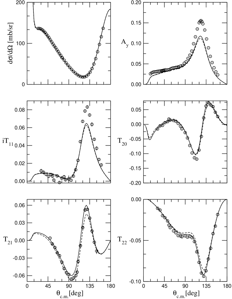
Figure 5: Differential cross section, proton vector-analyzing power $A_{y}$, and four deuteron tensor polarization observables for $pd$ elastic scattering at $T_{c.m.}=$6.66 MeV as function of the c.m. scattering angle. The dashed and solid curves are obtained with the AV18 and AV18/UIX interaction models, respectively. The experimental differential cross section and $A_{y}$ data are from Ref. sag94 , while the experimental tensor-analyzing power data are from Ref. gru83 .

For example, various $p-d$ observables at $T_{c.m.}=6.66$ MeV predicted by the AV18/UIX model are shown in Fig. 5 and are found to be in good agreement with the available experimental data sag94 ; gru83 . The large discrepancy observed for the $A_{y}$ and ${\rm i}\,T_{11}$ observables (the “$A_{y}$-puzzle”) is connected to a not well understood deficiency of the nuclear interaction, most likely of present TNI models. Resolving this “$A_{y}$-puzzle” is a current and important area of research.

The bound-state wave function $\Psi_{3}^{JJ_{z}}$ ($J=1/2$) is just given by the term $\Psi_{C}^{JJ_{z}}$, which is expanded as in Eq. (94). In this case, the functions $u_{\alpha,K}(\rho)$ are determined by the Rayleigh-Ritz variational principle, applying the boundary conditions $u_{\alpha,K}(\rho\rightarrow\infty)\rightarrow 0$. In practice, they are expanded in terms of Laguerre polynomials multiplied for an exponential factor Kie93 ; Kie94 . The number of channels included in such an expansion will be denoted by $N_{c}({\rm b.s.})$ in the following. The PHH expansion is very accurate also for bound states, as shown, for example, in Ref. nogga , where a very detailed comparison with the results of the Faddeev calculations of the Bochum group has been performed.

In the following, it is convenient to use the wave function $\Psi_{{{\bm{p}}},\sigma_{2}\sigma}^{(+)}$, where $\sigma_{2}$ and $\sigma$ are the spin projections of the $d$ and $N$ clusters, and ${{\bm{p}}}$ their relative momentum in the incident channel. It is given by

$$\Psi_{{{\bm{p}}},\sigma_{2}\sigma}^{(+)}=4\pi\sum_{SS_{z}}\langle 1\sigma_{2},\frac{1}{2}\sigma|SS_{z}\rangle\sum_{LMJJ_{z}}{\rm i}^{L}\>\langle SS_{z},LM|JJ_{z}\rangle Y_{LM}^{*}({\hat{{\bm{p}}}}){{\rm e}^{{\rm i}\sigma_{L}}\over 2{\rm i}}\Psi_{1+2}^{LSJJ_{z}}\>\>\>,$$ (99)

where $\sigma_{L}$ is the Coulomb phase shift. For a $nd$ state the factor ${\rm e}^{{\rm i}\sigma_{L}}$ is omitted. The wave function $\Psi_{{{\bm{p}}},\sigma_{2}\sigma}^{(+)}$ satisfies outgoing wave boundary conditions, and is normalized to unit flux, while the two- and three-nucleon bound-state wave functions are normalized to one.

In earlier papers Viv96 ; Viv00 , the sum over $J$ in Eq. (99) was truncated to a given value $J_{\rm max}=7/2$, since the analysis was limited to study low-energy radiative capture ($T_{c.m.}\leq 2$ MeV). In the present work, we extend the calculations to higher energy. In this case, it is necessary to take into account also the contribution of higher partial waves. For large values of $J$, and correspondingly large values of $L$, the centrifugal barrier between the deuteron and the third nucleon prevents the two clusters to approach each other. The corresponding $\Psi_{1+2}^{LSJJ_{z}}$ of either the $nd$ or $pd$ state can therefore be approximated to describe the free or Coulomb-distorted motion. For $pd$ as an example,

$$\Psi_{1+2}^{LSJJ_{z}}\rightarrow\Psi_{1+2,{\rm free}}^{LSJJ_{z}}={1\over\sqrt{3}}\sum_{{\rm cyclic}\>ijk}\Big{[}[\phi_{d}({{\bm{x}}}_{i})\otimes\chi_{i}]_{S^{\prime}}\otimes Y_{L^{\prime}}({\hat{{\bm{y}}}}_{i})\Big{]}_{JJ_{z}}{F_{L}(\eta,pr_{i})\over pr_{i}}\qquad J>J_{\rm max}\>\>\>.$$ (100)

In the calculation of transition matrix elements, we found it convenient to divide the sum over $J$ in Eq. (99) as $\sum_{J}\rightarrow\sum_{J\leq J_{\rm max}}+\sum_{J>J_{\rm max}}$. In the first sum, the wave functions $\Psi_{1+2}^{LSJJ_{z}}$ are calculated by taking into account the full PHH expansion (the effect of increasing the number $N_{c}({\rm s.s.})$ of scattering state channels is studied for a few selected cases in Sec. V.1). In the second sum, the wave function $\Psi_{1+2}^{LSJJ_{z}}$ is approximated as in Eq. (100). In this case, the sum over $L$ can be evaluated analytically to reconstruct the Coulomb distorted “plane wave” describing $p-d$ motion. In summary,

$$\Psi_{{{\bm{p}}},\sigma_{2}\sigma}^{(+)}=4\pi\sum_{J\leq J_{\rm max},J_{z}}\sum_{SS_{z}}\langle\frac{1}{2}\sigma,1\sigma_{2}|SS_{z}\rangle\sum_{LM}{\rm i}^{L}\>\langle SS_{z},LM|JJ_{z}\rangle Y_{LM}^{*}({\hat{{\bm{p}}}}){{\rm e}^{{\rm i}\sigma_{L}}\over 2{\rm i}}\Psi_{1+2}^{LSJJ_{z}}+\Delta\Psi_{{{\bm{p}}},\sigma_{2}\sigma}^{(+)}\>\>\>,$$ (101)

where

$$\Delta\Psi_{{{\bm{p}}},\sigma_{2}\sigma}^{(+)} = \sum_{{\rm cyclic}\>ijk}\phi_{d}^{1\sigma_{2}}({{\bm{x}}}_{i})\chi_{i}^{{1\over 2}\sigma}\;\psi_{c}^{(+)}({{\bm{p}}},{{\bm{r}}}_{i})-4\pi\sum_{J\leq J_{\rm max},J_{z}}\sum_{SS_{z}}\langle\frac{1}{2}\sigma,1\sigma_{2}|SS_{z}\rangle\times$$ (102)

$$\times\sum_{LM}{\rm i}^{L}\>\langle SS_{z},LM|JJ_{z}\rangle Y_{LM}^{*}({\hat{{\bm{p}}}}){{\rm e}^{{\rm i}\sigma_{L}}\over 2{\rm i}}\Psi_{1+2,{\rm free}}^{LSJJ_{z}}\>\>\>,$$

and $\psi^{(+)}_{c}({{\bm{p}}},{{\bm{r}}})$ is the solution of the three-dimensional Schrödinger equation with the pure Coulomb potential behaving asymptotically as a plane plus a scattered wave, i.e.

$$\psi^{(+)}_{c}({{\bm{p}}},{{\bm{r}}})=e^{{\rm i}{{\bm{p}}}\cdot{{\bm{r}}}}{\rm e}^{-\pi\eta/2}\Gamma(1+{\rm i}\eta){}_{1}F_{1}(-{\rm i}\eta,{\rm i}pr-{\rm i}{{\bm{p}}}\cdot{{\bm{r}}})\>\>\>.$$ (103)

Here, ${}_{1}F_{1}$ is the confluent hypergeometric function. The function given in Eq. (103) reduces simply to the plane wave for $\eta=0$ ($nd$ case).

V Results

In the present section we report results for the $np$ radiative capture at thermal neutron energies and deuteron photodisintegration cross section at low energy, the $nd$ and $pd$ radiative capture reactions at c.m. energy $T_{c.m.}=$ 2–20 MeV, and the isoscalar and isovector magnetic form factors of ³H and ³He. In the next two subsections, we report the results for the $pd$ radiative capture at $T_{c.m.}=2.0$ and $3.33$ MeV, for which there are very accurate cross-section and polarization data Goe92 ; Smi99 . One reason for doing so is to test the quality of the bound and scattering wave functions, in particular by studying the rate of convergence of calculated reduced-matrix elements (RMEs) with respect to the number of channels included in the PHH expansions of these wave functions.

The second reason is to make a comparative study of the different current operator models introduced in the present work. Some of these models satisfy the CCR exactly, others do so only approximately. The question is how critical is this lack of current conservation and how large are the contributions of three-body currents induced by the trinucleon interaction.

In Ref. Viv00 significant deviations were obtained between the measured and calculated tensor observables $T_{20}$ and $T_{21}$ in $p$$d$ radiative capture. That earlier study was carried out with a current operator including, in addition to one-body, two- and three-body terms, denoted as old-ME and old-TCO in the present work. As shown below, most of the observed discrepancy between theory and experiment can be traced back to the fact that the current of Ref. Viv00 was not exactly conserved.

In the other subsections, the predictions obtained with the new models of the electromagnetic current will be compared with data in $A$=2 and 3 nucleon systems.

V.1 Test of the wave functions

In order to test the PHH wave functions, we have performed a series of calculations of the $pd$ capture reaction at $T_{c.m.}=2$ MeV with a Hamiltonian including the Argonne $v_{18}$ (AV18) two-nucleon Wir95 and Urbana IX (UIX) three-nucleon Pud95 interactions (the AV18/UIX Hamiltonian model). The model for the electromagnetic current chosen for this test is the new “full” one, i.e. including the one-body, the new-ME two-body and the ME three-body terms. More precisely,

$${\bm{j}}^{\rm full-new}({\bm{q}})=\sum_{i}{\bm{j}}_{i}({\bm{q}})+\sum_{i<j}[{\bm{j}}^{MI,{\rm new}}_{ij}({\bm{q}})+{\bm{j}}^{MD}_{ij}({\bm{q}})]+\sum_{{\rm cyclic}\ ijk}{\bm{j}}^{ME}_{j;ki}({\bm{q}})\ ,$$ (104)

where ${\bm{j}}^{MI,{\rm new}}_{ij}({\bm{q}})$ and ${\bm{j}}^{ME}_{j;ki}({\bm{q}})$ are given in Eqs. (65) and (74), respectively. The RMEs are computed from the matrix elements

$$j_{\sigma_{3}\lambda J_{z}}^{LSJ}(p,q)=\langle\Psi_{3}^{{1\over 2}\sigma_{3}}|\hat{\epsilon}^{*}_{\lambda}({\bf q})\cdot{\bf j}^{\dagger}({\bf q})|\Psi^{LSJJ_{z}}_{1+2}\rangle\ ,$$ (105)

where $\epsilon_{\lambda}({\bf q})$, $\lambda=\pm 1$, are the spherical components of the photon polarization vector Viv96 .

Some of the most relevant RMEs for $pd$ capture at this energy are the electric dipoles $\overline{\cal E}^{LSJ}_{1}$ induced by transitions between $p$$d$ states in relative orbital angular momentum quantum number $L=1,3$ and the ³He state. Here $S=1/2,3/2$ are the channel spin quantum numbers obtained by coupling the spins of the proton and deuteron, and $\vec{J}=\vec{L}+\vec{S}$ (the notation and definition used for the RMEs are those of Ref. Viv00 ). The calculated RMEs are listed in Table 1. In the different calculations, we varied the number of channels included in the bound and scattering PHH wave functions, namely the value $N_{c}$ in the first sum of Eq. (94). The channels are ordered for increasing values of $l_{\alpha}+L_{\alpha}$, $l_{\alpha}$ and $L_{\alpha}$ being the orbital angular momentum of the pair and of the third nucleon with respect to the pair, respectively. In this analysis, the values for $N_{K}(\alpha)$ were taken large enough to have full convergence with respect to the order $K$ of Jacobi polynomials.

Table 1: RMEs ($\times 10^{3}$) for $pd$ radiative capture at $T_{\rm c.m.}=2$ MeV obtained with the AV18/UIX Hamiltonian and the new-ME two- and three-body currents. For the exact definition of the RMEs, see Eq. (4.26) of Ref. Viv00 . In the table, $N_{c}({\rm b.s.})$ ($N_{c}({\rm s.s.})$) indicates the number of channels included in the expansion of the bound state (scattering state of given $J$ and parity $\pi$).

State $J={1\over 2}^{-}$
RME	$(N_{c}({\rm b.s.}),N_{c}({\rm s.s.}))$	(12,10)	(18,10)	(18,14)	(18,18)
$\overline{\cal E}_{1}^{1{1\over 2}{1\over 2}}$		2.699	2.701	2.693	2.689
$\overline{\cal E}_{1}^{1{3\over 2}{1\over 2}}$		-0.134	-0.131	-0.203	-0.201
State $J={3\over 2}^{-}$
RME	$(N_{c}({\rm b.s.}),N_{c}({\rm s.s.}))$	(12,13)	(18,13)	(18,22)	(18,29)
$\overline{\cal E}_{1}^{1{1\over 2}{3\over 2}}$		2.725	2.733	2.714	2.711
$\overline{\cal E}_{1}^{1{3\over 2}{3\over 2}}$		0.103	0.103	0.089	0.089
$\overline{\cal E}_{1}^{3{3\over 2}{3\over 2}}$		0.075	0.075	0.126	0.127

First, consider the effect of the truncation of the PHH expansion in the description of the bound-state. The calculated binding energy for ³He with the AV18/UIX potential is $7.725$ ($7.741$) MeV after the inclusion of $N_{c}=12$ ($18$) channels in the PHH expansion. As can be seen by inspecting the two columns corresponding to the cases $N_{c}({\rm b.s.})=12$ and $18$, the changes in the values of the RMEs is at most 2%. We have checked that the inclusion of additional channels in the bound state wave function produces tiny changes in the binding energy (less than 10 keV) and negligible changes in all the RMEs.

Next, consider the convergence with respect to $N_{c}({\rm s.s.})$, the number of channels in the scattering wave functions. In general, the dependence of the calculated RMEs on $N_{c}({\rm s.s.})$ is weak. The only exceptions are the RMEs due to the inhibited $E_{1}$ transitions proceeding through the spin-channel $S=3/2$ states, which require the inclusion of a fairly large number of channels. In general, the convergence can be checked by looking at $Nd$ elastic scattering phase-shifts $\delta^{LSJ}$ obtained with the given value of $N_{c}({\rm s.s.})$. Let us consider, for example, the transitions to the $J={1\over 2}^{-}$ $pd$ scattering state. The elastic phase shift $\delta^{LSJ}$ for the state $L=1$, $S=1/2$ and $J=1/2$ were found to have the values $\delta^{1{1\over 2}{1\over 2}}=-7.393^{\circ}$, $-7.366^{\circ}$ and $-7.365^{\circ}$ for $N_{c}({\rm s.s.})=10$, $14$ and $18$ channels, respectively. The corresponding changes in $\overline{\cal E}_{1}^{1{1\over 2}{1\over 2}}$ are given in the first row of Table 1 and are very small. On the other hand, for the $L=1$, $S=3/2$ and $J=1/2$ state, the elastic phase-shift turns out to be $\delta^{1{3\over 2}{1\over 2}}=21.666^{\circ}$, $22.318^{\circ}$ and $22.319^{\circ}$ for $N_{c}({\rm s.s.})=10$, $14$ and $18$ channels, respectively. The elastic phase-shift here has a fairly large change passing from $N_{c}=10$ to $N_{c}=14$, due to the appearance of important channels in the PHH expansion. The corresponding change in $\overline{\cal E}_{1}^{1{3\over 2}{1\over 2}}$ is very significant, as can be seen by inspecting the second row of Table 1. However, by adding more channels, the elastic phase-shift and the corresponding capture RMEs show only tiny changes. A similar check has been performed for all the other scattering states included in the calculation.

We have verified by direct calculation that differences between the observables obtained by using the RMEs computed with the two largest values of $N_{c}$ are completely negligible. Note that in the present paper the bound and scattering wave functions have been obtained on a more extended grid and with more PHH components than in previous publications Viv96 ; Viv00 . However, this better accuracy in the wave functions has produced negligible changes in the $nd$ and $pd$ capture observables for $T_{c.m.}\leq 2$ MeV, which were the focus of Refs. Viv96 ; Viv00 .

For the range of energies considered here, the most important $Nd$ scattering waves are those with $J^{\pi}={1\over 2}^{\pm}$, ${3\over 2}^{\pm}$ and ${5\over 2}^{\pm}$. For these scattering states a fairly large number of channels has to be included in the PHH expansion of the “core” wave function $\Psi_{3}^{JJ_{z}}$. Scattering states with higher values of $J^{\pi}$ give very small contributions. As mentioned before, we have retained the full PHH expansion in the states up to $J_{\rm max}=7/2$. For larger values of $J$, the scattering wave function has been approximated as in Eq. (100).

V.2 Test of the two- and three-body current models

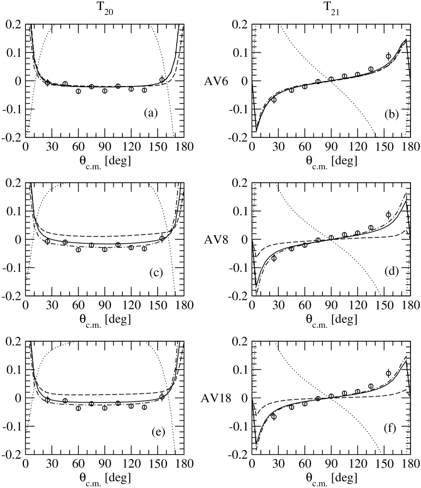
Figure 6: Deuteron tensor polarization observables $T_{20}$ and $T_{21}$ for $pd$ radiative capture at $T_{c.m.}=$2 MeV as function of the c.m. $\gamma$-$p$ scattering angle, obtained with the AV6, AV8 and AV18 Hamiltonian models. Dotted, dashed and solid lines are obtained with only one-body current, with one- and old-ME two-body currents and with one- and $LP$-MS two-body currents, respectively. The results obtained in long-wavelength approximation are also shown (dotted-dashed lines). The experimental data are from Ref. Smi99 .

We have calculated the $T_{20}$ and $T_{21}$ observables at $T_{c.m.}=$ 2 MeV using the Argonne $v_{6}$ (AV6) Wir02 , the Argonne $v_{8}$ (AV8) Pud97 and AV18 two-nucleon interaction. The AV6 interaction is momentum-independent, while the momentum-dependence of the AV8 is due only to the spin-orbit operator. The results are shown in Fig. 6.

First, let us consider the calculations performed with the AV6 interaction, reported in panels (a) and (b). The dotted curves are obtained by including only the one-body current contributions. The dashed curves are obtained when the contributions of the old-ME two-body currents of Refs. Viv96 ; Viv00 ; Mar98 , see Eq. (64), are added to the one-body ones. The solid curves are obtained including instead the two-body current contributions calculated within the MS scheme and using the linear path ($LP$-MS, see Sec. II.2). Finally, the dotted-dashed curves are obtained in the long-wavelength-approximation (LWA). We observe that in this case there is no significant difference between the old-ME, $LP$-MS, LWA and experimental results. For this potential $v^{p}_{ij}=0$, and therefore the old-ME and new-ME two-body current models coincide. We see that the current derived from the momentum-independent part of the interaction using either the ME or $LP$-MS schemes are almost equivalent. This is not too surprising, given the small photon energy involved in the process, $q\approx 0.035$ fm^-1, see discussion in Sec. II.2.

Next, let us consider the calculations performed with the AV8 and AV18 interactions, reported in panels (c)–(f). Now, the solid curves are obtained using the new-ME scheme, namely the current ${\bm{j}}^{MI,{\rm new}}_{ij}({\bm{q}})$ given in Eq. (65). Note that the old-ME two-body current model results (dashed lines) are in significant disagreement with the LWA ones and the experimental data, as can be seen by inspecting panels (c)–(f) of Fig. 6. This is not the case for the new-ME results (those obtained with the $LP$-MS model have not been reported, since they are practically coincident with the solid lines). This indicates that the current operator ${\bm{j}}_{ij}^{ME}({\bm{q}};v^{p})$ used in Refs. Viv96 ; Viv00 ; Mar98 and in earlier studies, which does not satisfy exactly the CCR with the momentum-dependent terms of the two-nucleon interaction, contain spurious contributions.

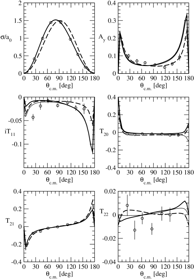
Figure 24: Differential cross section, proton vector analyzing power, and the four deuteron tensor polarization observables for $pd$ radiative capture at $T_{c.m.}=$3.33 MeV as function of the c.m. $\gamma$-$p$ scattering angle, obtained with the AV18 Hamiltonian model and the one- plus new-ME two-body nuclear current operators. The dashed, thin-solid and thick-solid lines are obtained with no Coulomb interaction in the bound- and scattering-state wave functions, with Coulomb interaction only in the bound-state wave function, and with inclusion of the Coulomb interaction both in the bound- and in the scattering-state wave functions, respectively. The experimental data are from Ref. Goe92 .

This conclusion is supported by another observation. Using the bound and scattering wave functions derived from the AV18 interaction, but taking into account ${\bm{j}}_{ij}^{ME}({\bm{q}};v^{0})$ only, a good description of the observables $T_{20}$ and $T_{21}$ is still obtained (see, for example, Fig. 24 of Ref. Golak00 ). The inclusion of the old-model current ${\bm{j}}_{ij}^{ME}({\bm{q}};v^{p})$ produces quite large effects on the RMEs and spoils such an agreement with the data Viv00 . On the other hand, the contribution of the momentum-dependent part of the interaction is noticeably smaller than that one produced by $v^{0}_{ij}$, as can be seen, for example, in studies of the binding energies of the light nuclei Wir91 . Therefore, one can reasonably expect that also $|{\bm{j}}_{ij}({\bm{q}};v^{p})|\ll|{\bm{j}}_{ij}({\bm{q}};v^{0})|$. The current ${\bm{j}}_{ij}^{LP}({\bm{q}};v^{p})$, constructed in order to properly satisfy the CCR with $v^{p}_{ij}$, gives correctly a small contribution to the RMEs, and now the $T_{20}$ and $T_{21}$ at $T_{c.m.}=2$ MeV are well reproduced. The same happens at higher energies, as will be shown below.

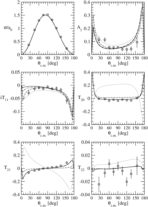
Figure 7: Differential cross section, proton vector analyzing power, and the four deuteron tensor polarization observables for $pd$ radiative capture at $T_{c.m.}=$2 MeV as function of the c.m. $\gamma$-$p$ scattering angle, obtained with the AV18 Hamiltonian model. The dotted curves are obtained with only one-body currents, the dashed and dotted-dashed curves retain, in addition, the contributions from the MI two-body operators ${\bm{j}}_{ij}^{{\rm MI},{\rm old}}({\bm{q}})$ and ${\bm{j}}_{ij}^{{\rm MI},{\rm new}}({\bm{q}})$ (see Eqs. (64) and (65)), respectively. The solid curves are obtained including, in addition to ${\bm{j}}_{ij}^{{\rm MI},{\rm new}}({\bm{q}})$, also the “model-dependent” two-body contributions. The experimental data are from Ref. Smi99 . In most of the panels, the dotted-dashed and solid curves are indistinguishable.

In order to verify that the agreement found in Ref. Viv00 for other observables is not spoiled, the differential cross section, proton vector analyzing power and the four deuteron tensor analyzing powers for $pd$ capture at $T_{c.m.}$= 2 and 3.33 MeV, calculated with the AV18 two-nucleon interaction, are compared with the experimental data of Refs. Goe92 ; Smi99 in Figs. 7 and 8. In the figures, the dotted curves are obtained with only one-body current contributions, the dashed and dotted-dashed curves are obtained using the one-body plus “model-independent” (MI) contributions ${\bm{j}}_{ij}^{MI,{\rm old}}({\bm{q}})$ and ${\bm{j}}_{ij}^{MI,{\rm new}}({\bm{q}})$, respectively, and the solid curve is obtained when, in addition to ${\bm{j}}_{ij}^{MI,{\rm new}}({\bm{q}})$, the “model-dependent” (MD) contributions (${\bm{j}}_{ij}^{MD}({\bm{q}})$), due to the $\rho\pi\gamma$ and $\omega\pi\gamma$ transition currents and to the current associated with the excitation of one intermediate $\Delta$ resonance, are retained (“full” model). The contributions from the isospin-symmetry-breaking operators described in Sec. II.3 are also included, but have been found to be completely negligible.

With the new model for the nuclear current operator, there is an overall good agreement between experimental results and theoretical predictions, except for the i$T_{11}$ observable at small c.m. angles. Furthermore, comparing the solid and dotted-dashed lines, we conclude that the MD contributions are typically very small, the only exception being those for i$T_{11}$. As will be shown below, this observable is also influenced by three-body current contributions. The improved description of the measured $T_{20}$ and $T_{21}$ observables, discussed earlier, is evident.

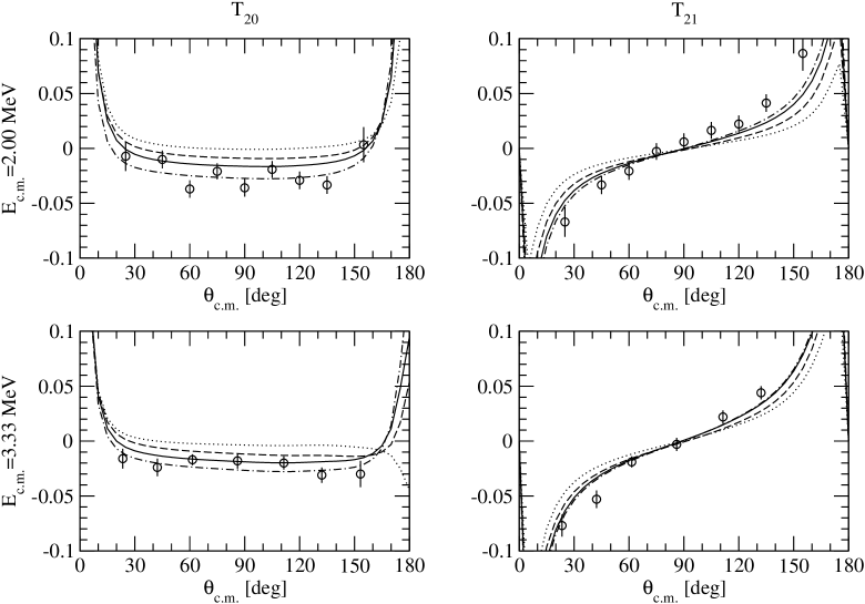
Figure 9: Deuteron tensor polarization observables $T_{20}$ and $T_{21}$ for $pd$ radiative capture at $T_{c.m.}=$2 and 3.33 MeV as function of the c.m. $\gamma$-$p$ scattering angle, obtained with the AV18/UIX Hamiltonian model. The dotted, dashed and solid curves correspond to the calculation with one- and two-body currents only, with the three-body current obtained within the TCO approach, with the three-body current ${\bm{j}}_{ijk}^{ME}({\bm{q}})$ obtained within the ME scheme (see Eqs. (89) and (74)). The results obtained in LWA are also shown (dotted-dashed curves). The experimental data are from Refs. Goe92 ; Smi99 .

We now turn our attention to the three-body current. In Fig. 9 the tensor spin observables $T_{20}$ and $T_{21}$ for $pd$ radiative capture at $T_{c.m.}=$ 2 and 3.33 MeV are calculated using the wave functions from the AV18/UIX Hamiltonian model. The dotted curves correspond to calculations with one- and new-ME two-body currents only. The dashed curves have been obtained by including, in addition, the three-body current of Ref. Mar98 , obtained within the old-TCO approach. Finally, the solid curves correspond to calculations with one-, new-ME two-body and new-ME three-body current ${\bm{j}}_{ijk}^{ME}({\bm{q}})$ of Eqs. (89) and (74), obtained within the ME scheme. The results obtained with the three-body current operator calculated within the $LP$-MS scheme (${\bm{j}}_{ijk}^{LP}({\bm{q}})$ of Eq. (85)) are not shown, because they coincide with those obtained with the ME method. Finally, the dotted-dashed curves are the LWA results. Inspection of Fig. 9 indicates that, if we use the wave functions obtained from a Hamiltonian including a TNI but disregard the corresponding three-body current (dotted curves), there is a significant disagreement with the data. The use of the old-TCO three-body current improves partially the description of the data, but only including the new-ME (or, equivalently, the $LP$-MS) three-body current leads to a satisfactory agreement with the experimental data and LWA results, especially for the $T_{21}$ observable.

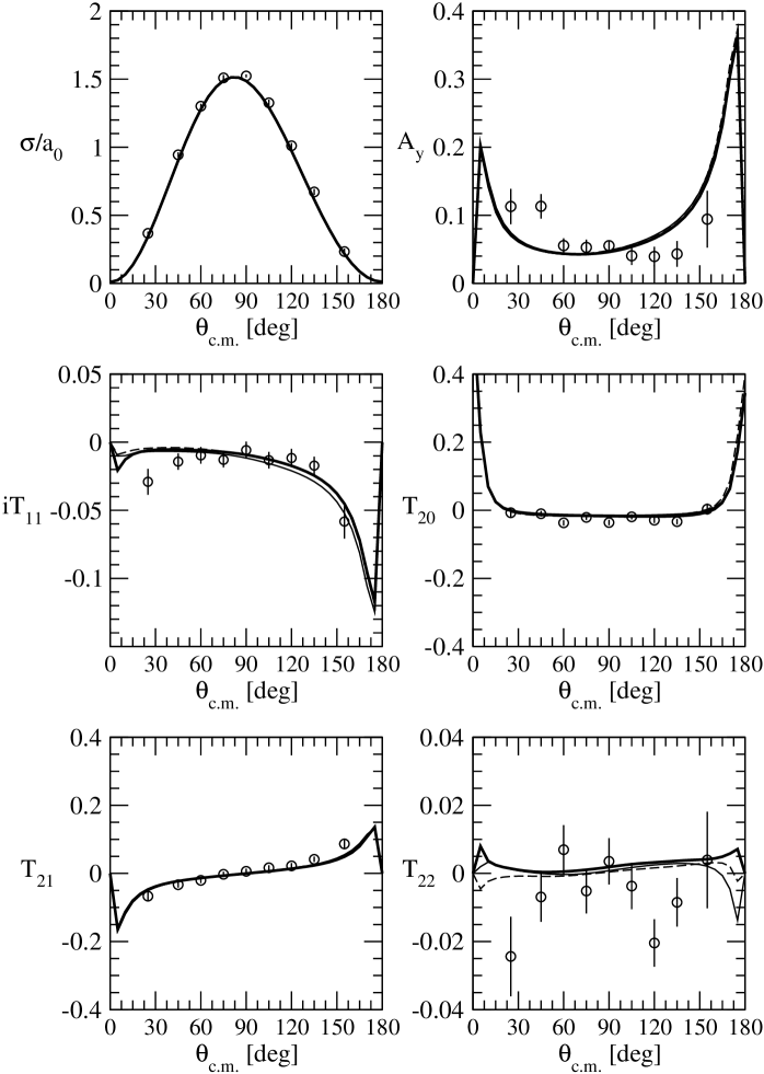
Figure 10: Differential cross section, proton vector analyzing power, and the four deuteron tensor polarization observables for $pd$ radiative capture at $T_{c.m.}=$2 MeV as function of the c.m. $\gamma$-$p$ scattering angle, obtained with the AV18 (dashed lines), AV18/TM (thin solid lines) and AV18/UIX (thick solid lines) Hamiltonian models. The model for the nuclear current operator include one-, two-, and three-body contributions and they satisfy the CCR with each given Hamiltonian. The experimental data are from Ref. Smi99 . In most of the panels, the three curves are indistinguishable.

Finally, the differential cross section and the spin polarization observables for $pd$ capture at $T_{c.m.}$= 2 and 3.33 MeV, calculated with the AV18, AV18/UIX and AV18/TM Hamiltonian models are compared with the experimental data of Refs. Goe92 ; Smi99 in Figs. 10 and 11. The dashed lines are the AV18 results obtained using the corresponding wave functions and including, in addition to the one-body current operator, the new-ME current ${\bm{j}}_{ij}^{MI,{\rm new}}({\bm{q}})$ and the MD current ${\bm{j}}_{ij}^{MD}({\bm{q}})$. The thin solid curves are obtained with the Hamiltonian including the AV18 and the Tucson-Melbourne (TM) Coo79 TNI (AV18/TM model). In this case, the current includes the one-body, the new-ME and MD two-body and the new-ME three-body currents (constructed to satisfy the CCR with the AV18/TM Hamiltonian). The thick solid lines are finally obtained with the AV18/UIX Hamiltonian, and include the corresponding set of one-, two-, and three-body currents in the new-ME scheme. As the figures suggest, there are no significant differences between the AV18, AV18/TM and AV18/UIX results, except for some tiny effects in the ${\rm i}T_{11}$ observable.

V.3 Magnetic structure of $A$=3 nuclei

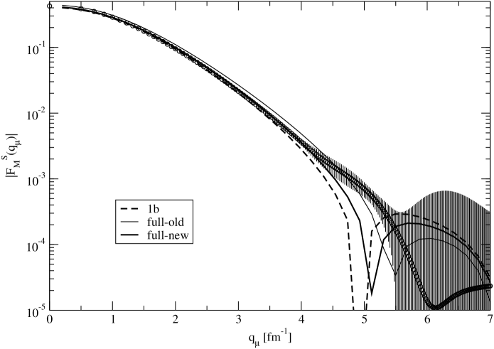
Figure 12: The isoscalar combination of the ³He and ³H magnetic form factors, obtained with single nucleon currents (1b), and with the inclusion of two- and three-body currents in the new model summarized in Secs. II.4 and III.3 (full-new). Also listed are the results obtained with the old-ME two-body and old-TCO three-body currents of Ref. Mar98 (full-old). The experimental data are from Ref. Col65 ; McC77 ; Sza77 ; Arn78 ; Dun83 ; Ott85 ; Jus85 ; Bec87 ; Amr94 .

The isoscalar and isovector combinations of the magnetic moments and form factors of ³He and ³H are given in Table 2 and Figs. 12 and 13, respectively. The nuclear wave functions have been calculated using the the AV18/UIX Hamiltonian model. The results labeled “1b” are obtained retaining only the one-body current operator, those labeled “full-new” are obtained including, in addition, the new-ME two-body current contributions and the three-body current contributions calculated in the ME scheme. Also listed, are the results obtained with the old-ME two-body and old-TCO three-body currents, as in Ref. Mar98 , labeled “full-old”. These last results are slightly different from those reported in Ref. Mar98 , due to the present use of more accurate trinucleon wave functions. The experimental data are from Refs. tunl ; Col65 ; McC77 ; Sza77 ; Arn78 ; Dun83 ; Ott85 ; Jus85 ; Bec87 ; Amr94 .

Note that: (i) the “full-old” and “full-new” results for the isoscalar and isovector magnetic moments differ by less than 1 % and are very close to the experimental data; (ii) the experimental results for the isovector magnetic form factor are fairly well reproduced for momentum transfer $q_{\mu}\leq 3.5$ fm^-1, and the “full-new” curve is slightly closer to the experimental data in the region $q_{\mu}\geq 4$ fm^-1 than the “full-old” curve; (iii) the “full-new” curve for the isoscalar magnetic form factor is closer to the experimental data than the “full-old” curve in the region $q_{\mu}\leq 4$ fm^-1; (iv) the “full-new” curves for the isoscalar and isovector form factors are in disagreement with the data for $q_{\mu}\geq$ 4–4.5 fm^-1, and the discrepancy between theory and experiment in this region remains unresolved. However, the experimental data for the isoscalar magnetic form factor have large errors at high $q_{\mu}$ values.

Table 2: Isoscalar and isovector combinations $\mu_{S}$ and $\mu_{V}$ of the ³He and ³H magnetic moments, in nuclear magnetons, compared with experimental data. The results labeled “1b” are obtained with single-nucleon currents only, those labeled “full-new” retain in addition two- and three-body currents in the new model summarized in Secs. II.4 and III.3. Also listed are the results obtained with the old-ME two-body and old-TCO three-body currents of Ref. Mar98 (“full-old”). The experimental data are from Ref. tunl .

	$\mu_{S}$	$\mu_{V}$
1b	0.407	2.165
Full-new	0.414	2.539
Full-old	0.442	2.557
Expt.	0.426	2.553

V.4 $A$=2 radiative capture reaction and deuteron photodisintegration

The calculated values for the ¹H($n$,$\gamma$)²H cross section at thermal neutron energies with the old- and new-ME models of the current are listed in Table 3. The AV18 two-nucleon interaction is used.

Table 3: Total cross section in mb for the $n$$p$ radiative capture, calculated using the AV18 two-nucleon interaction. The results labeled “1b” are obtained with single-nucleon currents only, those labeled “1b+2b-MI(old-ME)” and “1b+2b-MI(new-ME)” retain in addition model-independent two-body currents in the old-ME and new-ME model summarized in Secs. II.4. The results labeled “full-old” and “full-new” are obtained by adding the contributions of the model-dependent two-body currents to the “1b+2b-MI(old-ME)” and “1b+2b-MI(new-ME)” results, respectively. The experimental value is from Ref. Mug81 .

	$\sigma$(mb)
1b	304.6
1b+2b-MI(old-ME)	326.1
1b+2b-MI(new-ME)	324.7
Full-old	334.2
Full-new	332.7
Expt.	332.6 $\pm$ 0.7

The small difference between the results obtained with the old- and new-ME models is due to differences in the isovector structure of the two-body currents from the momentum dependent terms of the AV18. The result with the new-ME model happens to be in perfect agreement with the experimental value reported in Ref. Mug81 .

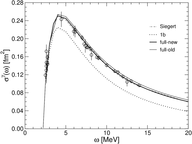
Figure 14: The deuteron photodisintegration cross sections obtained with one-body current (1b) and with, in addition, the old (full-old) or new (full-new) models for two-body currents are compared to experimental values. Also shown are the results obtained by using the Siegert form for the $E_{1}$ transition. The experimental data are from Refs. Bis50 ; Sne50 ; Col51 ; Car51 ; Bir85 ; Mor89 ; DeG92 .

The deuteron photodisintegration cross sections up to 20 MeV photon energies obtained in impulse approximation and with the full-old and full-new ME current models are shown in Fig. 14, along with the experimental data Bis50 ; Sne50 ; Col51 ; Car51 ; Bir85 ; Mor89 ; DeG92 . Also shown in Fig. 14 are the predictions in which the dominant $E_{1}$ transitions connecting the deuteron and $n$$p$ triplet $P$-waves are calculated using the Siegert form for the $E_{1}$ operator, valid in the LWA limit. Again, differences between the results obtained with the new- and old-ME current models is to be attributed mostly to differences in the isovector currents originating from the momentum dependence of the AV18. Indeed, these terms ensure that the new-ME current is exactly conserved, and make the corresponding results essentially identical to the Siegert predictions.

V.5 $A$=3 radiative capture reactions

We report here the results for the radiative capture reactions ²H($n,\gamma$)³H and ²H($p,\gamma$)³He, obtained with the AV18/UIX Hamiltonian model.

V.5.1 The ²H($n,\gamma$)³H radiative capture reaction

At thermal energies the $nd$ capture reaction proceeds through $S$-wave capture predominantly via magnetic dipole transitions from the initial doublet $J$=1/2 and quartet $J$=3/2 $nd$ scattering states. In addition, there is a small contribution due to an electric quadrupole transition from the initial quartet state.

The results for the thermal energy cross section and photon polarization parameter are presented in Table 4, along with the experimental data JBB82 ; Kea88 . As can be seen by inspection of the table, the cross section calculated with single-nucleon currents is approximately a factor of 2 smaller than the measured value. A previous calculation Viv96 gave $\sigma_{T}({\rm 1b})=0.223$ mb, very close to the results presented in the first row of Table 4. Inclusion of the model-independent new-ME two-body currents leads to a value of $\sigma_{T}$ 10% smaller than obtained earlier with the MI old-ME currents of Ref. Viv96 . By adding the model-dependent two-body current, an estimate of $\sigma_{T}=0.523$ mb is obtained. This value is to be compared with the corresponding result $\sigma_{T}=0.558$ mb obtained in Ref. Viv96 . The use of the present MI two-body current operators therefore leads to an estimate closer to the experimental datum $\sigma_{T}=0.508\pm 015$ mb JBB82 . However, the addition of the three-body currents, which give a rather sizable contribution as can be seen from the row labeled “full-new” in Table 4, brings the total cross section to $\sigma_{T}=0.556$ mb. The 9% slight overprediction is presumably due to the model-dependent currents associated with the $\Delta$ excitations. Fortunately, at $T_{c.m.}>1$ MeV, this MD current gives a negligible contribution to the cross section and the other polarization observables, as already shown in Figs. 7 and 8.

Table 4: Cross section (in mb) and photon polarization parameter $R_{c}$ of the reaction ²H($n,\gamma$)³H for the AV18/UIX potential model at thermal neutron energy. The results labeled “1b” are obtained with single-nucleon currents only, those labeled “1b+2b-MI(old-ME)” and “1b+2b-MI(new-ME)” retain in addition MI two-body currents in the old-ME and new-ME scheme, respectively. The results labeled “$\ldots$+2b-MD” are obtained by adding the model-dependent two-body currents to the single-nucleon and the MI new-ME two-body currents. Finally, the results labeled “full-new” are obtained by including to the latter model also the the contribution of the ME three-body currents, defined in Sec. III.3. The experimental values for $\sigma_{T}$ and $R_{c}$ are from Refs. JBB82 ; Kea88 , respectively.

Current component	$\sigma_{T}$	$R_{c}$
1b	0.227	–0.061
1b+2b-MI(old-ME)	0.462	–0.446
1b+2b-MI(new-ME)	0.418	–0.429
$\ldots$+2b-MD	0.523	–0.469
Full-new	0.556	–0.476
Expt.	$0.508\pm 0.015$	–$0.42\pm 0.03$

The photon polarization parameter is very sensitive to two-body currents (for its definition in terms of RMEs, see Ref. Viv96 ). For example, for the AV18/UIX Hamiltonian, their inclusion produces roughly a six-fold increase, in absolute value, of the single-nucleon prediction. Also in this case, we find a 13% overprediction (in absolute value) of this parameter. The small reduction of $|R_{c}|$, found when the new-ME model for the two-body current is used, is compensated by the inclusion of the three-body currents.

At higher energies, there exist several measurements of the unpolarized differential cross section for both the radiative capture process ²H($n,\gamma$)³H mitev86 and for the “time-reversed” process ³H($\gamma,n$)²H bosch64 ; faul81 ; skopik81 ; koseik66 ; pfeiffer68 . In the c.m. system and at low energies, the unpolarized cross sections are related by the principle of detailed balance

$$\left({d\sigma_{\rm photo}\over d\Omega}\right)_{c.m.}={3\over 2}\left({p\over q}\right)^{2}\left({d\sigma_{\rm capt}\over d\Omega}\right)_{c.m.}\>\>\>,$$ (106)

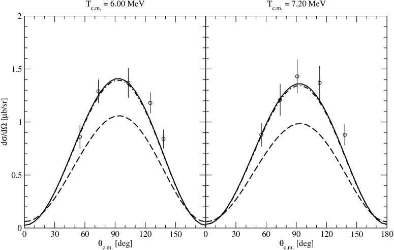
Figure 15: Differential cross section in $\mu$b/sr for $nd$ radiative capture at $T_{c.m.}=$6 MeV and 7.2 MeV as function of the c.m. $\gamma$-$n$ scattering angle, obtained with the AV18/UIX Hamiltonian model. The dashes curves have been obtained using the single-nucleon current only. The dotted-dashed curves have been obtained with the inclusion of the new-ME two-body currents. Finally, the solid curves have been obtained by adding the ME three-body current. The experimental data are from Ref. mitev86 .

where $q$ and $p$ are the $\gamma$ and the relative $nd$ momenta, respectively. In Figure 15, we compare our predictions for $(d\sigma_{\rm capt}/d\Omega)_{c.m.}$ with the experimental results of Ref. mitev86 , which is the only direct measurement of the ²H($n,\gamma$)³H differential cross section. The dashed curves represent the results obtained with the inclusion of the single-nucleon current only, the dotted-dashed curves are obtained with one- and new-ME two-body contributions (both MI and MD), and the solid curves represent the “full-new” result, obtained including, in addition to the one-body and above-mentioned two-body currents, also the ME three-body current contributions. At these energies the process is dominated by $E_{1}$ transitions between the $nd$ $P$-wave states and the ³H ground state, as can be inferred from the bell-shape of the curves. The slight distortion of the peak is due to non-negligible contributions from $E_{2}$ RMEs, coming, in particular, from the $J=3/2,5/2$ states with $S=3/2$. Our “full-new” calculation reproduces quite well the experimental data, with some differences at large angles. As will be shown below, this has some consequences for the so-called fore-aft asymmetry, discussed in Sec. V.5.3.

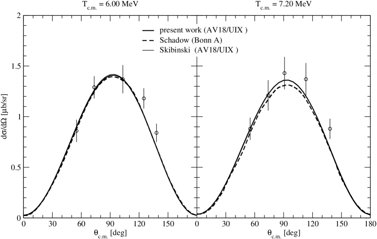
Figure 16: Differential cross section in $\mu$b/sr for $nd$ radiative capture at $T_{c.m.}=$6 MeV and 7.2 MeV as function of the c.m. $\gamma$-$n$ scattering angle, obtained in present work (thick solid curves) and in Ref. Skib03 (thin solid curves) using the AV18/UIX potential model. The two curves are practically indistinguishable. The dashed curves are the results of Ref. Schad01 obtained with the Bonn A potential model Mac87 . The experimental data are from Ref. mitev86 .

In Fig. 16, we compare our “full-new” results with those obtained in Refs. Schad01 ; Skib03 . In Ref. Skib03 , the same potential model (AV18/UIX) as in present work has been used, but the authors adopt a slightly different current model (they do not consider ${\bm{j}}_{ij}^{ME}({\bm{q}};v^{p})$, ${\bm{j}}_{ij}^{MD}({\bm{q}})$ and the three-body current). In Ref. Schad01 , the exchange currents are taken into account using Siegert’s theorem, and a different two-body potential model has been used (Bonn A Mac87 ), without any inclusion of three-nucleon forces. As can be seen by inspecting Fig. 16, the three theoretical calculations are practically the same, with some differences with results of Ref. Schad01 at $T_{c.m.}=7.20$ MeV. This difference is likely due to the use of a different potential model, which slightly underestimates the ³H binding energy.

In addition to unpolarized cross sections, there are also a few analyzing-power angular distribution data mitev86 , but they have large error bars, and therefore we have decided not to perform a comparison for this observable.

V.5.2 The ²H($p,\gamma$)³He radiative capture reaction

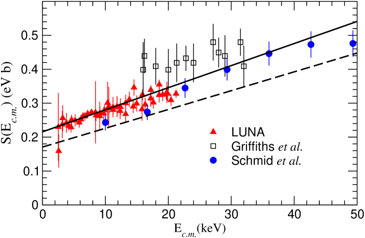
Figure 17: The $S$ factor of the ²H($p,\gamma$)³He reaction, obtained with the AV18/UIX Hamiltonian model and with the one-body current only (dashed line), and with the one-, two- and three-body current (solid line) is compared with the experimental results from Refs. Lun02 ; Gri63 ; Sch95 ; Sch96 .

In Fig. 17 we present the results for the astrophysical $S$ factor of the ²H($p,\gamma$)³He radiative capture reaction at thermal energies. This quantity is defined as

$$S(T_{c.m.})=T_{c.m.}\,\sigma_{T}(T_{c.m.})\,{\rm e}^{2\pi\alpha/v_{rel}}\ ,$$ (107)

where $T_{c.m.}$ is the $pd$ c.m. kinetic energy, $\sigma_{T}(T_{c.m.})$ is the total cross section, $\alpha$ is the fine structure constant, and $v_{rel}$ is the $pd$ relative velocity. The experimental data are from Refs. Lun02 ; Gri63 ; Sch95 ; Sch96 . The solid curve represents the “full-new” result, obtained including, in addition to the one-body currents, also the new-ME two-body current contributions and the three-body current contributions calculated in the ME scheme. The dashed curve represents the result obtained with the inclusion of the single-nucleon current only. Here, no significant difference has been seen between the results obtained with the present model for the nuclear current operator and the “old” one of Refs. Viv96 ; Viv00 . The agreement between the theoretical predictions and the experimental data, especially the very recent LUNA data Lun02 , is excellent. In particular, the calculated $S$ factor at zero energy is 0.219 eV b Viv00 , in very nice agreement with the LUNA result of 0.216$\pm$0.010 eV b.

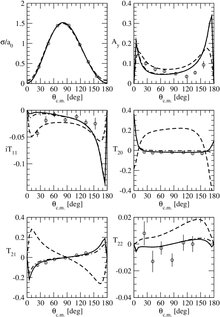
Figure 19: Same as Fig. 18 at $T_{c.m.}=$3.33 MeV. The experimental data are from Ref. Goe92 .

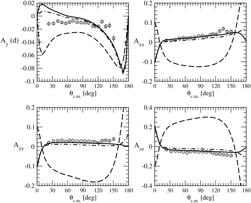
Figure 20: Four deuteron tensor polarization observables for $pd$ radiative capture at $T_{c.m.}=$5.83 MeV as function of the c.m. $\gamma$-$p$ scattering angle, obtained with the AV18/UIX Hamiltonian model. The same notation as in Fig. 18 is used for the different lines. The experimental data are from Ref. Aki01 .

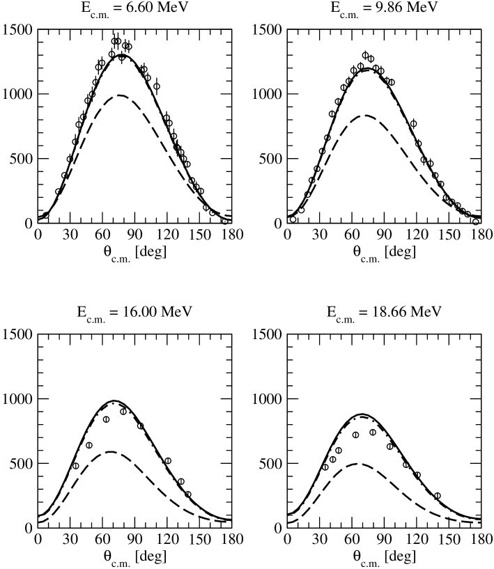
Figure 21: Differential cross section in $\mu$b/sr for $pd$ radiative capture up to $T_{c.m.}=$18.66 MeV as function of the c.m. $\gamma$-$p$ scattering angle, obtained with the AV18/UIX Hamiltonian model. The same notation as in Fig. 18 is used for the different lines. The experimental data are from Ref. Bel70 for $T_{c.m.}=$6.60 and 9.86 MeV, and from Ref. Ang83 for the other cases.

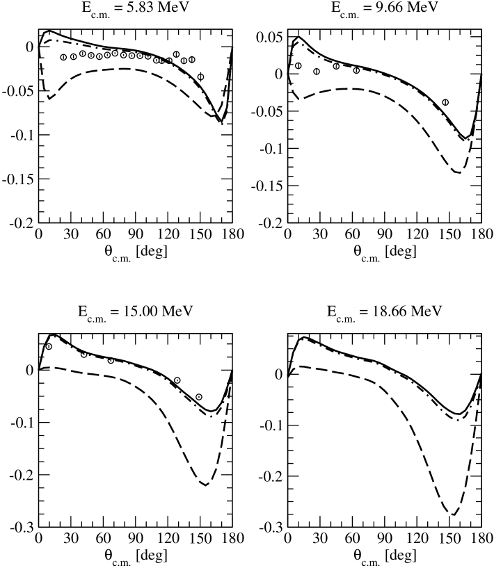
Figure 22: Deuteron vector analyzing power $A_{y}(d)$ for $pd$ radiative capture up to $T_{c.m.}=$18.66 MeV as function of the c.m. $\gamma$-$p$ scattering angle, obtained with the AV18/UIX Hamiltonian model. The same notation as in Fig. 18 is used for the different lines. The experimental data are from Ref. Aki01 for $T_{c.m.}=$5.83 MeV and from Refs. Jou86 ; Joupc for $T_{c.m.}=$9.66 and 15.00 MeV. No data at $T_{c.m.}=18.66$ MeV are available in literature up to now.

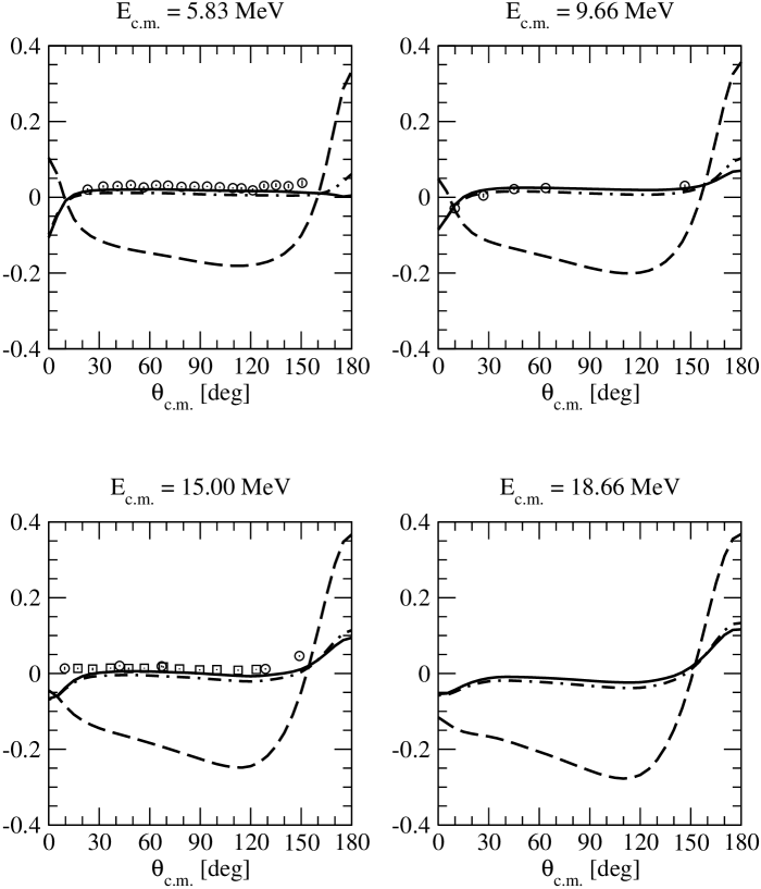
Figure 23: Deuteron tensor analyzing power for $pd$ radiative capture up to $T_{c.m.}=$18.66 MeV as function of the c.m. $\gamma$-$p$ scattering angle, obtained with the AV18/UIX Hamiltonian model. The same notation as in Fig. 18 is used for the different lines. The experimental data are from Ref. Aki01 for $T_{c.m.}=$5.83 MeV, from Refs. Jou86 ; Joupc for $T_{c.m.}=$9.66, and from Refs. Jou86 ; Joupc ; Ank98 for $T_{c.m.}=$15.00 MeV. No data at $T_{c.m.}=18.66$ MeV are available in literature up to now.

There exist several measurements of ²H($p$,$\gamma$),³He observables between $T_{c.m.}=2$ and $20$ MeV. In Figs. 18–23, we compare the predictions obtained with our new model of the current with a selected set of observables. In all these figures, the dashed lines are obtained with only one-body contributions, the dotted-dashed ones are obtained with one- and new-ME two-body contributions (MI+MD), the solid curves are the “full” results with, in addition, also three-body contributions, obtained in the ME scheme. For completeness, the predicted angular distributions of the differential cross section $\sigma/a_{0}$, proton vector analyzing power $A_{y}$, and deuteron vector and tensor analyzing powers i$T_{11}$, $T_{20}$, $T_{21}$, $T_{22}$, at $T_{c.m.}=2$ and 3.33 MeV are again given in Figs. 18 and 19. Note that these two c.m. energies are just below and above the deuteron breakup threshold. We can conclude that: (i) an overall nice description for all the observables has been obtained, with the only exception of the i$T_{11}$ deuteron polarization observable at small angles; (ii) some small three-body currents effects are noticeable, especially in the $T_{20}$ and $T_{21}$ deuteron tensor observables.

The predicted angular distributions of the deuteron vector and tensor analyzing powers $A_{y}$(d), $A_{xx}$, $A_{yy}$, $A_{zz}$, at $T_{c.m.}=5.83$ are given in Fig. 20. The experimental data are from Ref. Aki01 . Comments similar to those above can be made in this case too.

The differential cross section $d\sigma/d\Omega$ and the deuteron vector- and tensor-analyzing powers $A_{y}$(d) and $A_{yy}$ are given in Figs. 21, 22 and 23 for four different c.m. energies. The differential cross section is nicely reproduced by theory at $T_{c.m.}=$6.60 and 9.86 MeV, while some discrepancies are present at $T_{c.m.}=$16.00 and 18.66 MeV. However, it should be pointed out that these data sets are quite old, and new experimental studies of this process in this energy range would be very useful. The $A_{y}$(d) observables are poorly reproduced at small angles for $T_{c.m.}=$5.83 and 9.66 MeV. However, at $T_{c.m.}=$15.00 MeV, the discrepancy between theory and experiment seems to disappear. It would be interesting to continue this comparison at higher values of $T_{c.m.}$. The $A_{yy}$ observables are nicely reproduced in the whole range of $T_{c.m.}$. Some small discrepancies are present at small angles for $T_{c.m.}=$15.00 MeV. It is important to note, however, that the $A_{y}$(d) and $A_{yy}$ observables are obtained dividing for the differential cross section, which is close to zero at small and large values of the c.m. angle. In view of this, the agreement between theory and experiment for the $A_{y}$(d) and $A_{yy}$ observables should be considered satisfactory in the whole range of c.m. angles.

Finally, in Fig. 24 we study the importance of including the Coulomb interaction in the bound- and scattering-state wave functions. In fact, the $T_{c.m.}=$3.33 MeV differential cross section and vector- and tensor-analyzing powers are calculated using the AV18 nuclear Hamiltonian and one-body plus new-ME two-body currents. The Coulomb interaction is included both in the bound- and scattering-state wave functions (thick-solid lines), in the bound- but not in the scattering-state wave functions (thin-solid lines), and neither in the bound- nor in the scattering-state wave functions (dashed lines). The Coulomb interaction plays a small but significant role, particularly in the differential cross section.

V.5.3 The fore-aft asymmetry

A quantity of particular interest, both for historical reasons and for purposes of comparison with data, is the so-called fore-aft asymmetry in the angular distribution of the cross section. This quantity is defined according to

$$a_{s}={\sigma(54.7^{\circ})-\sigma(125.3^{\circ})\over\sigma(54.7^{\circ})+\sigma(125.3^{\circ})}\>\>\>,$$ (108)

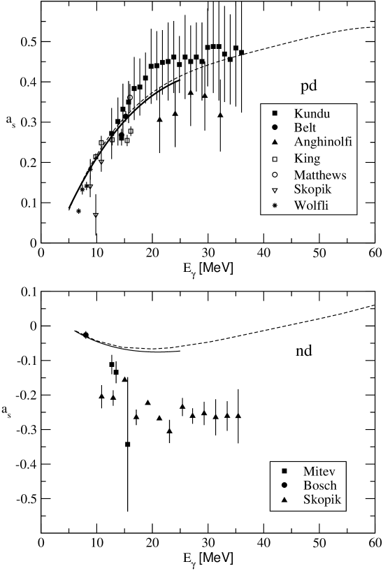
Figure 25: Fore-aft asymmetry for $pd$ and $nd$ radiative capture as function of the $\gamma$ energy, obtained with the AV18/UIX Hamiltonian model and the “full-new” current (solid lines). The results of the calculation of Ref. Schad01 have been also reported (dashed lines). The $pd$ experimental data are from Refs. wolfli66 ; Bel70 ; kundu71 ; matt74 ; skopik79 ; Ang83 ; skopik83 ; king84 , and the $nd$ experimental data are from Refs. bosch64 ; skopik81 ; mitev86 .

where $\sigma(\theta_{c.m.})=(d\sigma_{\rm capt}/d\Omega)_{c.m.}$ and $\theta_{c.m.}$ is the $\gamma$-$N$ scattering angle. The ²H($p,\gamma$)³He and ²H($n,\gamma$)³H asymmetries resulting from our calculation and from that of Ref. Schad01 are compared with existing data in Fig. 25.

The $pd$ asymmetry is well reproduced by the calculation (it is a consequence of the good agreement between the theoretical and experimental cross section angular distributions, shown in Fig. 21). On the other hand, there are large differences between the theoretical and experimental $nd$ asymmetries. These differences could be due to problems in the analysis of the data to extract the experimental values of $a_{s}$. For example, the experimental asymmetry comes out mainly from the measurement taken at the largest angle (see Fig. 15). Note that for other values of $\theta_{c.m.}$, good agreement is obtained between theory and experiment. There are also inconsistencies between the asymmetries given in Refs. skopik81 ; mitev86 , therefore it is likely that these discrepancies are due to experimental problems. However, if experimentally confirmed, this problem could be of relevance, since the present calculations seem unable to predict $|a_{s}(nd)|>0.1$.

VI Summary and Conclusions

We have investigated two different approaches for constructing conserved two- and three-body electromagnetic currents: one is based on meson-exchange mechanisms, while the other uses minimal substitution in the explicit and implicit–via the isospin exchange operator–momentum dependence of the two- and three-nucleon interactions. In the meson exchange model developed by Riska and collaborators Ris85a ; Sch89 ; Ris85b ; Ris85c and used in earlier studies Viv96 ; Viv00 ; Car90 ; Sch89 ; Sch91 , some of the terms associated with the isospin- and momentum-dependent components of the two-nucleon interaction were ignored, since, due to their short range character, they were expected to give negligible contributions. The resulting currents, however, were not strictly conserved. This limitation is removed in the present work. We have also shown how the two-body currents obtained in the meson-exchange framework (more precisely, their longitudinal part) can be derived in the minimal-substitution scheme, originally developed by Sachs Sac48 , by selecting a specific path in the space-exchange operator. Lastly, we have constructed a realistic model for the three-body electromagnetic current satisfying the current conservation relation with the Urbana or Tucson-Melbourne three-nucleon interactions.

A variety of observables have been calculated to test the present model of nuclear current operator. In particular, for the $A$=3 nuclear systems, cross sections as well as polarization observables have been calculated and compared with the corresponding experimental results in the energy range 0–20 MeV.

In general, the contributions due to the new two- and three-body currents—from the momentum dependence of the two-nucleon interaction and from the three-nucleon interaction, respectively—are found to be numerically small. However, they resolve the discrepancies between theory and experiment obtained in earlier studies Viv00 for some of the polarization parameters measured in $p$$d$ radiative capture, specifically the tensor polarizations $T_{20}$ and $T_{21}$. These contributions also reduce the overprediction of the $n$$d$ radiative capture cross section at thermal neutron energy from the 15 % obtained in Ref. Viv96 to the current 9 %.

In conclusion, (i) the predictions for the $n$$p$ radiative capture and low-energy deuteron photodisintegration Sch04 , and for the magnetic form factors of ³He and ³H, have remained essentially unchanged from those reported in previous studies Mar98 ; (ii) a satisfactory agreement between theory and experiment for $p$$d$ radiative capture observables above deuteron breakup threshold up to 20 MeV has been found, in particular for the tensor observables. Some discrepancies, however, persist in the vector polarization observables at forward angles.

Appendix A

In this appendix we show how the meson-exchange (ME) two-body currents (rather, their longitudinal components) from the static part of the two-nucleon interaction can be derived in the minimal substitution (MS) scheme by selecting a specific path in the space-exchange operator. To this end, we first write

$$v_{2,ij}\,\bm{\tau}_{i}\cdot\bm{\tau}_{j} = \sum_{a}(v^{a}_{PS,ij}+v^{a}_{V,ij}+v^{a}_{VS,ij})\,\bm{\tau}_{i}\cdot\bm{\tau}_{j}\ ,$$ (109)

$$v^{a}_{PS,ij} = -f^{2}_{PS,a}({\bm{\sigma}}_{i}\cdot{\bm{\nabla}}_{i})({\bm{\sigma}}_{j}\cdot{\bm{\nabla}}_{j})\,Y_{a}(r)\ ,$$ (110)

$$v^{a}_{V,ij} = -f^{2}_{V,a}({\bm{\sigma}}_{i}\times{\bm{\nabla}}_{i})\cdot({\bm{\sigma}}_{j}\times{\bm{\nabla}}_{j})\,Y_{a}(r)\ ,$$ (111)

$$v^{a}_{VS,ij} = f^{2}_{VS,a}\,Y_{a}(r)\ ,$$ (112)

$$Y_{a}(r) = \frac{{\rm e}^{-m_{a}r}}{4\pi\,r}\ ,$$ (113)

where $f_{PS,a}$, $f_{V,a}$, $f_{VS,a}$ and $m_{a}$ are appropriate parameters, see Eqs. (26)–(28). The two-body current which satisfies the current conservation relation with $v_{2,ij}$ is then written in MS scheme as

$${\bm{j}}_{ij}({\bm{q}})=\sum_{a}\bigg{[}{\bm{j}}^{a}_{ij}({\bm{q}};PS)+{\bm{j}}^{a}_{ij}({\bm{q}};V)+{\bm{j}}^{a}_{ij}({\bm{q}};VS)\bigg{]}\ ,$$ (114)

where each term of the sum is given in Eq. (47), with $v_{2,ij}$ replaced by the corresponding $PS$, $V$ or $VS$ potential. First, we consider the simple spin-independent current ${\bm{j}}^{a}_{ij}({\bm{q}};VS)$: by choosing $\gamma_{ij}=-\gamma^{\prime}_{ji}$ and using Eq. (50), ${\bm{j}}^{a}_{ij}({\bm{q}};VS)$ can be written as

$${\bm{j}}^{a}_{ij}({\bm{q}};VS) = f^{2}_{VS,a}\,Y_{a}(r)\,{\bm{j}}^{a}_{ij}({\bm{q}})\ ,$$

$${\bm{j}}^{a}_{ij}({\bm{q}}) = G_{E}^{V}(q_{\mu}^{2})\,({\bm{\tau}}_{i}\times{\bm{\tau}}_{j})_{z}\,\int_{\gamma_{ij}}d{\bm{s}}\;{\rm e}^{{\rm i}{\bm{q}}\cdot{\bm{s}}}\ ,$$ (115)

where the path $\gamma_{ij}$ is selected to be

$${\bm{s}} = {\bm{R}}_{ij}-x{\bm{r}}_{ij}+{\rm i}\,r_{ij}\frac{{\hat{\bm{q}}}}{q}\bigg{[}L_{a}(x)-m_{a}\bigg{]}\ ,\hskip 28.45274pt-\frac{1}{2}\leq x\leq\frac{1}{2}\ ,$$

$${\bm{R}}_{ij} = \frac{1}{2}({\bm{r}}_{i}+{\bm{r}}_{j})\ ,\qquad{\bm{s}}\bigg{(}x=-{1\over 2}\bigg{)}={\bm{r}}_{i}\ ,\qquad{\bm{s}}\bigg{(}x=+{1\over 2}\bigg{)}={\bm{r}}_{j}\ ,$$

$$L_{a}(x) = \sqrt{m_{a}^{2}+q^{2}(\frac{1}{4}-x^{2})}\ .$$ (116)

It is straightforward to verify that $\sum_{a}{\bm{j}}^{a}_{ij}({\bm{q}};VS)$ reduces to ${\bm{j}}_{ij}({\bm{q}};VS)$ of Eq. (34), obtained in the ME scheme. In this case, both the longitudinal and transverse components of ${\bm{j}}_{ij}({\bm{q}};VS)$ are exactly reproduced.

Next, using Eq. (47), the $PS$ current reads

$${\bm{j}}_{ij}^{a}({\bm{q}};PS)=-f_{PS,a}^{2}\,{\bm{j}}_{ij}^{a}({\bm{q}})({\bm{\sigma}}_{i}\cdot{\bm{\nabla}}_{i})\,({\bm{\sigma}}_{j}\cdot{\bm{\nabla}}_{j})Y_{a}(r)\ ,$$ (117)

which can be rewritten as

$${\bm{j}}_{ij}^{a}({\bm{q}})({\bm{\sigma}}_{i}\cdot{\bm{\nabla}}_{i})\,({\bm{\sigma}}_{j}\cdot{\bm{\nabla}}_{j})Y_{a}(r) = ({\bm{\sigma}}_{i}\cdot{\bm{\nabla}}_{i})\,({\bm{\sigma}}_{j}\cdot{\bm{\nabla}}_{j})\,{\bm{j}}_{ij}^{a}({\bm{q}})\,Y_{a}(r)$$ (118)

$$- [({\bm{\sigma}}_{i}\cdot{\bm{\nabla}}_{i}){\bm{j}}_{ij}^{a}({\bm{q}})]\,[({\bm{\sigma}}_{j}\cdot{\bm{\nabla}}_{j})Y_{a}(r)]$$

$$- [({\bm{\sigma}}_{j}\cdot{\bm{\nabla}}_{j}){\bm{j}}_{ij}^{a}({\bm{q}})]\,[({\bm{\sigma}}_{i}\cdot{\bm{\nabla}}_{i})Y_{a}(r)]$$

$$- Y_{a}(r)({\bm{\sigma}}_{i}\cdot{\bm{\nabla}}_{i})\,({\bm{\sigma}}_{j}\cdot{\bm{\nabla}}_{j})\,{\bm{j}}_{ij}^{a}({\bm{q}})\ .$$

The $a$-meson in-flight current is again exactly reproduced (first line of Eq. (118)). However, only the longitudinal components of the contact terms are reproduced by Eq. (118) (second and third lines), since, via Eq. (49),

$$({\bm{\sigma}}_{i}\cdot{\bm{\nabla}}_{i})\,{\bm{q}}\cdot{\bm{j}}_{ij}^{a}({\bm{q}}) = -{\bm{\sigma}}_{i}\cdot{\bm{q}}\,{\rm e}^{{\rm i}{\bm{q}}\cdot{\bm{r}}_{i}}\ ,$$ (119)

$$({\bm{\sigma}}_{j}\cdot{\bm{\nabla}}_{j})\,{\bm{q}}\cdot{\bm{j}}_{ij}^{a}({\bm{q}}) = {\bm{\sigma}}_{j}\cdot{\bm{q}}\,{\rm e}^{{\rm i}{\bm{q}}\cdot{\bm{r}}_{j}}\ ,$$ (120)

and the last term of Eq. (118) vanishes when dotted with ${\bm{q}}$. Therefore, using Eqs. (118)–(120), Eq. (117) can be rewritten as

$${\bm{j}}^{a}_{ij}({\bm{q}};PS) = -f^{2}_{PS,a}\bigg{[}({\bm{\sigma}}_{i}\cdot{\bm{\nabla}}_{i})({\bm{\sigma}}_{j}\cdot{\bm{\nabla}}_{j}){\bm{j}}^{a}_{ij}({\bm{q}})\,Y_{a}(r)$$ (121)

$$+ G_{E}^{V}(q_{\mu}^{2})\,({\bm{\tau}}_{i}\times{\bm{\tau}}_{j})_{z}\,[{\rm e}^{{\rm i}{\bm{q}}\cdot{\bm{r}}_{i}}{\bm{\sigma}}_{i}\,({\bm{\sigma}}_{j}\cdot{\bm{\nabla}}_{j})-{\rm e}^{{\rm i}{\bm{q}}\cdot{\bm{r}}_{j}}{\bm{\sigma}}_{j}\,({\bm{\sigma}}_{i}\cdot{\bm{\nabla}}_{i})]\,Y_{a}(r)\bigg{]}$$

$$+ {\rm additional}\,\,{\rm transverse}\,\,{\rm terms}\ .$$

It would be interesting to evaluate the contributions of these additional transverse terms.

Similar considerations are valid for ${\bm{j}}_{ij}^{a}({\bm{q}};V)$, which can be written as

$${\bm{j}}^{a}_{ij}({\bm{q}};V) = -f^{2}_{V,a}\bigg{(}[({\bm{\sigma}}_{i}\times{\bm{\nabla}}_{i})\cdot({\bm{\sigma}}_{j}\times{\bm{\nabla}}_{j})]\,\,{\bm{j}}^{a}_{ij}({\bm{q}})\,Y_{a}(r)$$ (122)

$$\phantom{f^{2}_{V,a}}-({\bm{\sigma}}_{i}\times{\bm{\nabla}}_{i})\,\,[({\bm{\sigma}}_{j}\times{\bm{\nabla}}_{j})\cdot{\bm{j}}^{a}_{ij}({\bm{q}})]\,Y_{a}(r)$$

$$\phantom{f^{2}_{V,a}}-({\bm{\sigma}}_{j}\times{\bm{\nabla}}_{j})\,\,[({\bm{\sigma}}_{i}\times{\bm{\nabla}}_{i})\cdot{\bm{j}}^{a}_{ij}({\bm{q}})]\,Y_{a}(r)$$

$$- G_{E}^{V}(q_{\mu}^{2})\,({\bm{\tau}}_{i}\times{\bm{\tau}}_{j})_{z}\,[{\rm e}^{{\rm i}{\bm{q}}\cdot{\bm{r}}_{i}}{\bm{\sigma}}_{i}\times({\bm{\sigma}}_{j}\times{\bm{\nabla}}_{j})$$

$$\phantom{G_{E}^{V}(q_{\mu}^{2})\,({\bm{\tau}}_{i}\times{\bm{\tau}}_{j})_{z}}-{\rm e}^{{\rm i}{\bm{q}}\cdot{\bm{r}}_{j}}{\bm{\sigma}}_{j}\times({\bm{\sigma}}_{i}\times{\bm{\nabla}}_{i})]\,Y_{a}(r)\bigg{)}$$

$$+ {\rm additional}\,\,{\rm transverse}\,\,{\rm terms}\ .$$

Appendix B

We list here the two-body currents obtained with the MS method from the quadratic-momentum-dependent terms of the interaction. To this end, the $({\bm{L}}\cdot{\bm{S}})^{2}$ term is written as

$$({\bm{L}}\cdot{\bm{S}})^{2}=\frac{1}{2}{\bm{L}}^{2}-\frac{1}{2}\,{\bm{L}}\cdot{\bm{S}}+\frac{1}{4}\,\biggl{[}({\bm{\sigma}}_{i}\cdot{\bm{L}})\,({\bm{\sigma}}_{j}\cdot{\bm{L}})+({\bm{\sigma}}_{j}\cdot{\bm{L}})\,({\bm{\sigma}}_{i}\cdot{\bm{L}})\biggr{]}\ ,$$ (123)

and the potential functions associated with the ${\bm{L}}\cdot{\bm{S}}$ and ${\bm{L}}^{2}$ operators are re-defined accordingly, for example

$${\hat{v}_{b}}(r) = v_{b}(r)-\frac{1}{2}\,v_{bb}(r)\ ,$$ (124)

$${\hat{v}_{q}}(r) = v_{q}(r)+\frac{1}{2}\,v_{bb}(r)\ ,$$ (125)

and similarly for $v_{b\tau}(r)$ and $v_{q\tau}(r)$. The spin-orbit currents are then those given in Eqs. (57) and (60) with $v_{b}(r),v_{b\tau}(r)$ replaced by ${\hat{v}_{b}}(r),{\hat{v}_{b\tau}}(r)$.

For the ${\bm{L}}^{2}$ terms, given by

$$v_{q}={\bm{L}}^{2}\,[{\hat{v}_{q}}(r)+{\hat{v}_{q\sigma}}(r)\,{\bm{\sigma}}_{i}\cdot{\bm{\sigma}}_{j}+{\hat{v}_{q\tau}}(r)\,{\bm{\tau}}_{i}\cdot{\bm{\tau}}_{j}+{\hat{v}_{q\sigma\tau}}(r)\,{\bm{\sigma}}_{i}\cdot{\bm{\sigma}}_{j}{\bm{\tau}}_{i}\cdot{\bm{\tau}}_{j}]\ ,$$ (126)

using the linear path of Eq. (51), we find

$${\bm{j}}_{ij}({\bm{q}};LL) = \biggl{[}{\hat{v}_{q}}(r)+{\hat{v}_{q\sigma}}(r)\,{\bm{\sigma}}_{i}\cdot{\bm{\sigma}}_{j}\biggr{]}\biggl{[}\bigg{(}{\rm i}{\bm{r}}-{\bm{r}}\times{\bm{L}}\bigg{)}P_{-}+\frac{1}{4}({\bm{r}}\times{\bm{q}})\times{\bm{r}}\,P_{+}\biggr{]}\ ,$$ (127)

$${\bm{j}}_{ij}^{LP}({\bm{q}};LL\tau) = \frac{1}{2}\biggl{[}{\hat{v}_{q\tau}}(r)+{\hat{v}_{q\sigma\tau}}(r)\,{\bm{\sigma}}_{i}\cdot{\bm{\sigma}}_{j}\biggr{]}\biggl{[}\bigg{(}{\rm i}{\bm{r}}-{\bm{r}}\times{\bm{L}}\bigg{)}R_{-}+\frac{1}{4}({\bm{r}}\times{\bm{q}})\times{\bm{r}}R_{+}$$ (128)

$$+ {\rm i}\,G_{E}^{V}(q_{\mu}^{2})\,({\bm{\tau}}_{i}\times{\bm{\tau}}_{j})_{z}\,\{{\bm{L}}^{2}\,,\,{\bm{r}}f_{ij}({\bm{q}})\}\biggr{]}\ ,$$

where ${\bm{r}}\equiv{\bm{r}}_{ij}$, $\{\cdots\}$ denotes the anticommutator, and $f_{ij}({\bm{q}})$ is defined in Eq. (53). We have also defined

$$P_{\pm} = \epsilon_{i}{\rm e}^{{\rm i}{\bm{q}}\cdot{\bm{r}}_{i}}\pm\epsilon_{j}{\rm e}^{{\rm i}{\bm{q}}\cdot{\bm{r}}_{j}}\ ,$$ (129)

$$R_{\pm} = \eta_{i}{\rm e}^{{\rm i}{\bm{q}}\cdot{\bm{r}}_{i}}\pm\eta_{j}{\rm e}^{{\rm i}{\bm{q}}\cdot{\bm{r}}_{j}}\ ,$$ (130)

with $\epsilon_{i}$, $\epsilon_{j}$, $\eta_{i}$ and $\eta_{j}$ listed in Sec. II.

For the quadratic spin-orbit terms, given by

$${\hat{v}_{bb}} = \frac{1}{4}v_{bb}(r)\{{\bm{\sigma}}_{i}\cdot{\bm{L}}\,,\,{\bm{\sigma}}_{j}\cdot{\bm{L}}\}$$ (131)

$$+ \frac{1}{8}v_{bb\tau}(r)\{\{{\bm{\sigma}}_{i}\cdot{\bm{L}}\,,\,{\bm{\sigma}}_{j}\cdot{\bm{L}}\}\,,{\bm{\tau}}_{i}\cdot{\bm{\tau}}_{j}\}\ ,$$

again using the linear path, we find

$${\bm{j}}_{ij}({\bm{q}};bb) = \frac{1}{8}v_{bb}(r)\biggl{\{}P_{-}\,,\,[({\bm{\sigma}}_{i}\times{\bm{r}})\,({\bm{\sigma}}_{j}\cdot{\bm{L}})\,+\,({\bm{\sigma}}_{j}\times{\bm{r}})\,({\bm{\sigma}}_{i}\cdot{\bm{L}})\,]\biggr{\}}$$ (132)

$${\bm{j}}_{ij}^{LP}({\bm{q}};bb\tau) = \frac{1}{8}v_{bb\tau}(r)\biggl{[}\frac{1}{4}R_{+}\biggl{[}({\bm{\sigma}}_{j}\times{\bm{r}})\,\,[{\bm{q}}\cdot({\bm{\sigma}}_{i}\times{\bm{r}})]+({\bm{\sigma}}_{i}\times{\bm{r}})\,\,[{\bm{q}}\cdot({\bm{\sigma}}_{j}\times{\bm{r}})]\biggr{]}$$ (133)

$$+ R_{-}\biggl{[}({\bm{\sigma}}_{j}\times{\bm{r}})\,\,({\bm{\sigma}}_{i}\cdot{\bm{L}})+({\bm{\sigma}}_{i}\times{\bm{r}})\,\,({\bm{\sigma}}_{j}\cdot{\bm{L}})+{\rm i}({\bm{\sigma}}_{i}\cdot{\bm{\sigma}}_{j}){\bm{r}}-\frac{\rm i}{2}[{\bm{\sigma}}_{i}\,({\bm{\sigma}}_{j}\cdot{\bm{r}})+{\bm{\sigma}}_{j}\,({\bm{\sigma}}_{i}\cdot{\bm{r}})]\biggr{]}$$

$$+ {\rm i}\,G_{E}^{V}(q_{\mu}^{2})({\bm{\tau}}_{i}\times{\bm{\tau}}_{j})_{z}\biggl{\{}\{{\bm{\sigma}}_{i}\cdot{\bm{L}}\,,\,{\bm{\sigma}}_{j}\cdot{\bm{L}}\}\,,\,{\bm{r}}f_{ij}({\bm{q}})\biggr{\}}\biggl{]}\ .$$

Appendix C

Using Eq. (33), the configuration-space expressions for the exchange currents ${\bm{j}}_{ij}^{II}({\bm{k}}_{i},{\bm{k}}_{j};B)$ of Sec. III.1, $B=PS$ or $V$, are given by:

$${\bm{j}}_{ij}^{II}({\bm{q}};PS) = G_{E}^{V}(q_{\mu}^{2})({\bm{\tau}}_{i}\times{\bf T}_{j})_{z}$$ (134)

$$\Biggl{[} {\rm e}^{{\rm i}{\bm{q}}\cdot{\bm{r}}_{i}}\,g_{PS}(r){\bm{\sigma}}_{i}\,({\bf S}_{j}\cdot{\hat{\bm{r}}})\,+\,{\rm e}^{{\rm i}{\bm{q}}\cdot{\bm{r}}_{j}}\,g_{PS}(r){\bf S}_{j}\,({\bm{\sigma}}_{i}\cdot{\hat{\bm{r}}})$$

$$+ {\rm e}^{{\rm i}{\bm{q}}\cdot{\bm{R}}}\,\bigg{[}\frac{G_{PS,1}({\bm{r}})}{r^{2}}\,\bigg{(}{\bm{\sigma}}_{i}\,({\bf S}_{j}\cdot{\hat{\bm{r}}})+{\bf S}_{j}\,({\bm{\sigma}}_{i}\cdot{\hat{\bm{r}}})+{\hat{\bm{r}}}\,({\bm{\sigma}}_{i}\cdot{\bf S}_{j})\bigg{)}$$

$$\>\>\>\>\>\>\>\>\>\>\>\>+{\rm i}\frac{G_{PS,2}({\bm{r}})}{r}\,{\bm{\sigma}}_{i}\,({\bf S}_{j}\cdot{\bm{q}})-{\rm i}\frac{G_{PS,3}({\bm{r}})}{r}\,{\bf S}_{j}\,({\bm{\sigma}}_{i}\cdot{\bm{q}})$$

$$\>\>\>\>\>\>\>\>\>\>\>\>-{\rm i}\frac{G_{PS,4}({\bm{r}})}{r}\,{\hat{\bm{r}}}\,({\bm{\sigma}}_{i}\cdot{\hat{\bm{r}}})({\bf S}_{j}\cdot{\bm{q}})+{\rm i}\frac{G_{PS,5}({\bm{r}})}{r}\,{\hat{\bm{r}}}\,({\bm{\sigma}}_{i}\cdot{\bm{q}})({\bf S}_{j}\cdot{\hat{\bm{r}}})$$

$$\>\>\>\>\>\>\>\>\>\>\>\>-G_{PS,6}({\bm{r}})\,{\hat{\bm{r}}}\,({\bm{\sigma}}_{i}\cdot{\bm{q}})({\bf S}_{j}\cdot{\bm{q}})-\frac{G_{PS,7}({\bm{r}})}{r^{2}}\,{\hat{\bm{r}}}\,({\bm{\sigma}}_{i}\cdot{\hat{\bm{r}}})({\bf S}_{j}\cdot{\hat{\bm{r}}})\bigg{]}\,\Biggr{]}\ ,$$

$${\bm{j}}_{ij}^{II}({\bm{q}};V) = G_{E}^{V}(q_{\mu}^{2})({\bm{\tau}}_{i}\times{\bf T}_{j})_{z}$$ (135)

$$\Biggl{[} {\rm e}^{{\rm i}{\bm{q}}\cdot{\bm{r}}_{i}}\,g_{V}(r){\bm{\sigma}}_{i}\times({\bf S}_{j}\times{\hat{\bm{r}}})\,+\,{\rm e}^{{\rm i}{\bm{q}}\cdot{\bm{r}}_{j}}\,g_{V}(r){\bf S}_{j}\times({\bm{\sigma}}_{i}\times{\hat{\bm{r}}})$$

$$- {\rm e}^{{\rm i}{\bm{q}}\cdot{\bm{R}}}\,\bigg{[}\frac{G_{V,1}({\bm{r}})}{r^{2}}\,\bigg{(}({\bf S}_{j}\times{\hat{\bm{r}}})\times{\bm{\sigma}}_{i}+({\bm{\sigma}}_{i}\times{\hat{\bm{r}}})\times{\bf S}_{j}+2{\hat{\bm{r}}}\,({\bm{\sigma}}_{i}\cdot{\bf S}_{j})\bigg{)}$$

$$\>\>\>\>\>\>\>\>\>\>\>\>+{\rm i}\frac{G_{V,2}({\bm{r}})}{r}\,({\bf S}_{j}\times{\bm{q}})\times{\bm{\sigma}}_{i}-{\rm i}\frac{G_{V,3}({\bm{r}})}{r}\,({\bm{\sigma}}_{i}\times{\bm{q}})\times{\bf S}_{j}$$

$$\>\>\>\>\>\>\>\>\>\>\>\>-{\rm i}\frac{G_{V,4}({\bm{r}})}{r}\,{\hat{\bm{r}}}\,({\bm{\sigma}}_{i}\times{\hat{\bm{r}}})\cdot({\bf S}_{j}\times{\bm{q}})+{\rm i}\frac{G_{V,5}({\bm{r}})}{r}\,{\hat{\bm{r}}}\,({\bm{\sigma}}_{i}\times{\bm{q}})\cdot({\bf S}_{j}\times{\hat{\bm{r}}})$$

$$\>\>\>\>\>\>\>\>\>\>\>\>-G_{V,6}({\bm{r}})\,{\hat{\bm{r}}}\,({\bm{\sigma}}_{i}\times{\bm{q}})\cdot({\bf S}_{j}\times{\bm{q}})-\frac{G_{V,7}({\bm{r}})}{r^{2}}\,{\hat{\bm{r}}}\,({\bm{\sigma}}_{i}\times{\hat{\bm{r}}})\cdot({\bf S}_{j}\times{\hat{\bm{r}}})\bigg{]}$$

$$- \frac{1}{2}{\rm e}^{{\rm i}{\bm{q}}\cdot{\bm{R}}}\,\bigg{[}G_{V,2}({\bm{r}})\,({\bf S}_{j}\times{\bm{q}})\,\,{\bm{\sigma}}_{i}\cdot({\bm{q}}\times{\hat{\bm{r}}})+G_{V,3}({\bm{r}})\,({\bm{\sigma}}_{i}\times{\bm{q}})\,\,{\bf S}_{j}\cdot({\bm{q}}\times{\hat{\bm{r}}})$$

$$\>\>\>\>\>\>\>\>\>\>\>\>+{\rm i}\frac{G_{V,4}({\bm{r}})+G_{V,5}({\bm{r}})}{r}\,\bigg{(}({\bf S}_{j}\times{\hat{\bm{r}}})\,\,{\bm{\sigma}}_{i}\cdot({\hat{\bm{r}}}\times{\bm{q}})-({\bm{\sigma}}_{i}\times{\hat{\bm{r}}})\,\,{\bf S}_{j}\cdot({\hat{\bm{r}}}\times{\bm{q}})\bigg{)}$$

$$\>\>\>\>\>\>\>\>\>\>\>\>+{\rm i}\frac{G_{V,2}({\bm{r}})+G_{V,3}({\bm{r}})}{r}\,\bigg{(}{\bf S}_{j}\times({\bm{\sigma}}_{i}\times{\bm{q}})-{\bm{\sigma}}_{i}\times({\bf S}_{j}\times{\bm{q}})\bigg{)}\bigg{]}\Biggr{]}\ ,$$

where ${\bm{r}}={\bm{r}}_{i}-{\bm{r}}_{j}$, ${\hat{\bm{r}}}={\bm{r}}/r$, ${\bm{R}}=\frac{1}{2}({\bm{r}}_{i}+{\bm{r}}_{j})$, and

$$g_{PS}(r) = -\frac{1}{3\,r^{2}}\bigg{[}\int_{r}^{\infty}\,dr^{\prime}\,r^{\prime 2}\,v_{\sigma\tau}^{II}(r^{\prime})\,+\,2\,r^{3}\int_{r}^{\infty}\,dr^{\prime}\,\frac{v_{t\tau}^{II}(r^{\prime})}{r^{\prime}}\bigg{]}\ ,$$ (136)

$$g_{V}(r) = \frac{1}{3\,r^{2}}\bigg{[}\int_{r}^{\infty}\,dr^{\prime}\,r^{\prime 2}\,v_{\sigma\tau}^{II}(r^{\prime})\,-\,r^{3}\int_{r}^{\infty}\,dr^{\prime}\,\frac{v_{t\tau}^{II}(r^{\prime})}{r^{\prime}}\bigg{]}\ ,$$ (137)

$$G_{B,1}({\bm{r}}) = \int_{-1/2}^{1/2}dx\,{\rm e}^{-{\rm i}x{\bm{q}}\cdot{\bm{r}}}\bigg{[}E_{B}(x;r)\,-\,r\,\frac{d}{dr}\,E_{B}(x;r)\bigg{]}\ ,$$ (138)

$$G_{B,2}({\bm{r}}) = \int_{-1/2}^{1/2}dx\,{\rm e}^{-{\rm i}x{\bm{q}}\cdot{\bm{r}}}(\frac{1}{2}+x)\,E_{B}(x;r)\ ,$$ (139)

$$G_{B,3}({\bm{r}}) = \int_{-1/2}^{1/2}dx\,{\rm e}^{-{\rm i}x{\bm{q}}\cdot{\bm{r}}}(\frac{1}{2}-x)\,E_{B}(x;r)\ ,$$ (140)

$$G_{B,4}({\bm{r}}) = \int_{-1/2}^{1/2}dx\,{\rm e}^{-{\rm i}x{\bm{q}}\cdot{\bm{r}}}(\frac{1}{2}+x)\,\bigg{[}E_{B}(x;r)\,-\,r\,\frac{d}{dr}\,E_{B}(x;r)\bigg{]}\ ,$$ (141)

$$G_{B,5}({\bm{r}}) = \int_{-1/2}^{1/2}dx\,{\rm e}^{-{\rm i}x{\bm{q}}\cdot{\bm{r}}}(\frac{1}{2}-x)\,\bigg{[}E_{B}(x;r)\,-\,r\,\frac{d}{dr}\,E_{B}(x;r)\bigg{]}\ ,$$ (142)

$$G_{B,6}({\bm{r}}) = \int_{-1/2}^{1/2}dx\,{\rm e}^{-{\rm i}x{\bm{q}}\cdot{\bm{r}}}(\frac{1}{4}-x^{2})\,E_{B}(x;r)\ ,$$ (143)

$$G_{B,7}({\bm{r}}) = \int_{-1/2}^{1/2}dx\,{\rm e}^{-{\rm i}x{\bm{q}}\cdot{\bm{r}}}\bigg{[}3\,E_{B}(x;r)\,-\,3r\,\frac{d}{dr}\,E_{B}(x;r)\,+\,r^{2}\,\frac{d^{2}}{dr^{2}}\,E_{B}(x;r)\bigg{]}\ .$$ (144)

The functions $E_{B}(x;r)$ are defined as

$$E_{B}(x;r) = \sum_{a=1}^{N}\,\frac{g_{B,a}}{4\pi}\,{\rm e}^{-r\,L_{a}(x)}\ ,$$ (145)

$$L_{a}(x) = \sqrt{m_{a}^{2}\,+\,\frac{q^{2}}{4}\,\left(1-4x^{2}\right)}\ .$$ (146)

The coefficients $g_{B,a}$ are obtained by fitting the functions $v_{B}^{II}(k)$ of Sec. III.1, $B=PS,V$, with $\sum_{a=1}^{N}\,g_{B,a}/(k^{2}+m_{a}^{2})$ Sch89 .

Figure 1: Integration paths from position $i$ to position $j$ and vice versa for the integral of Eq. (40).

Figure 2: Feynman diagram representation of the three-body currents associated with $PS$- and $V$-meson exchanges. Thin, thick, dashed and wavy lines denote nucleons, $\Delta$-isobars, $a$-mesons, and photons, respectively.

Figure 3: Integration paths chosen to derive the three-body current operator of Eqs. (76) and (81).

Figure 4: Final position of particles $i$, $j$, and $k$ after that the product of the space exchange operators $P_{jk}P_{ij}$ is applied.

.

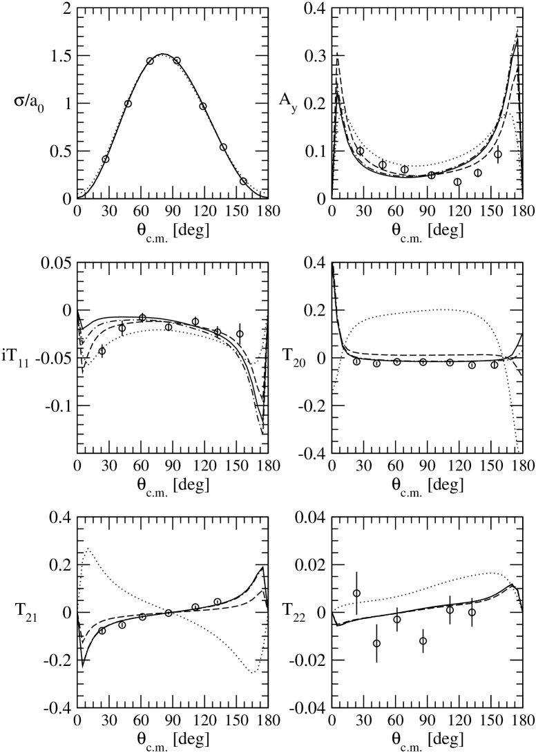
Figure 8: Same as Fig. 7 at $T_{c.m.}=$3.33 MeV. The experimental data are from Ref. Goe92 .

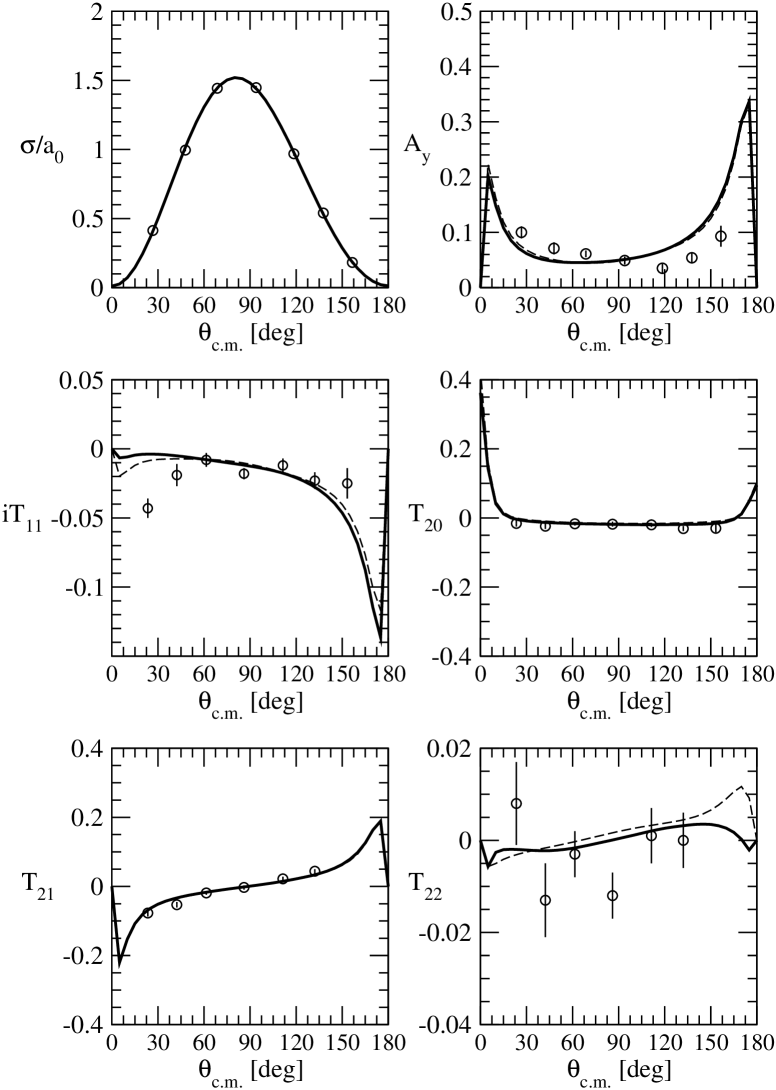
Figure 11: Same as Fig. 10 at $T_{c.m.}=$3.33 MeV. The dashed and thick solid lines are obtained with the AV18 and AV18/UIX Hamiltonian models, respectively. The experimental data are from Ref. Goe92 .

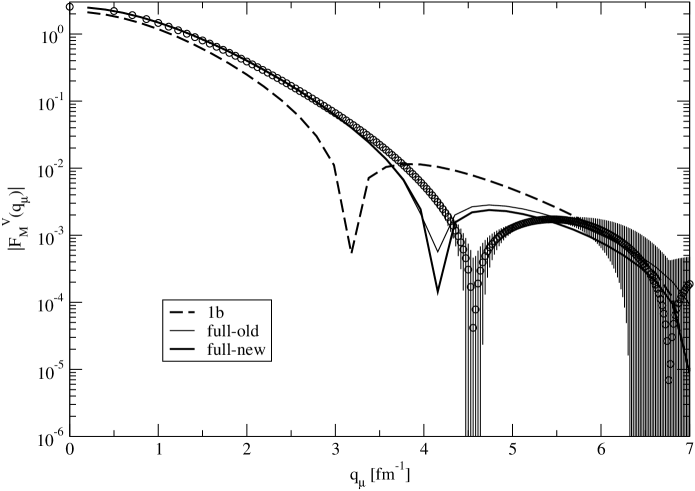
Figure 13: Same as Fig. 12, but for the isovector combination of the ³He and ³H magnetic form factors. The experimental data are from Ref. Col65 ; McC77 ; Sza77 ; Arn78 ; Dun83 ; Ott85 ; Jus85 ; Bec87 ; Amr94 .

Figure 18: Differential cross section, proton vector analyzing power, and the four deuteron tensor polarization observables for $pd$ radiative capture at $T_{c.m.}=$2 MeV as function of the c.m. $\gamma$-$p$ scattering angle, obtained with the AV18/UIX Hamiltonian model. The dashed, dotted-dashed and solid lines are obtained with one-body contributions, one- and new-ME two-body contributions, and one-, two- and three-body contributions. The experimental data are from Ref. Smi99 .

References

- (1) J. Carlson and R. Schiavilla, Rev. Mod. Phys. 70, 743 (1998).
- (2) M. Viviani, R. Schiavilla, and A. Kievsky, Phys. Rev. C 54, 534 (1996).
- (3) M. Viviani, A. Kievsky, L.E. Marcucci, S. Rosati, and R. Schiavilla, Phys. Rev. C 61, 064001 (2000).
- (4) L.E. Marcucci, D.O. Riska, and R. Schiavilla, Phys. Rev. C 58, 3069 (1998).
- (5) A. Kievsky, M. Viviani, and S. Rosati, Nucl. Phys. A551, 241 (1993).
- (6) A. Kievsky, M. Viviani, and S. Rosati, Nucl. Phys. A577, 511 (1994).
- (7) A. Kievsky, M. Viviani, and S. Rosati, Phys. Rev. C 64, 024002 (2001).
- (8) R.B. Wiringa, V.G.J. Stoks, and R. Schiavilla, Phys. Rev. C 51, 38 (1995).
- (9) B.S. Pudliner, V.R. Pandharipande, J. Carlson, and R.B. Wiringa, Phys. Rev. Lett. 74, 4396 (1995).
- (10) D.O. Riska, Phys. Scr. 31, 107 (1985).
- (11) J. Carlson, D.O. Riska, R. Schiavilla, and R.B. Wiringa, Phys. Rev. C 42, 830 (1990).
- (12) R. Schiavilla, V.R. Pandharipande, and D.O. Riska, Phys. Rev. C 40, 2294 (1989).
- (13) R. Schiavilla and D.O. Riska, Phys. Rev. C 43, 437 (1991).
- (14) R. Schiavilla, R.B. Wiringa, V.R. Pandharipande, and J. Carlson, Phys. Rev. C 45, 2628 (1992).
- (15) L.E. Marcucci, K.M. Nollett, R. Schiavilla, and R.B. Wiringa, ArXiv:nucl-th/0402078.
- (16) The LUNA Collaboration, Nucl. Phys. A706, 203 (2002).
- (17) M. Viviani, L.E. Marcucci, A. Kievsky, R. Schiavilla, and S. Rosati, Eur. Phys. J. A 17, 483 (2003).
- (18) L.E. Marcucci, M. Viviani, A. Kievsky, S. Rosati, and R. Schiavilla, Few-Body Syst. Suppl. 14, 319 (2003).
- (19) L.E. Marcucci, M. Viviani, A. Kievsky, S. Rosati, and R. Schiavilla, Few-Body Syst. Suppl. 15, 87 (2003).
- (20) F. Goeckner, W.K. Pitts, and L.D. Knutson, Phys. Rev. C 45, R2536 (1992).
- (21) A. Buchmann, W. Leidemann, and H. Arenhövel, Nucl. Phys. A 443, 726 (1985).
- (22) H. Arenhövel, F. Ritz, and T. Wilbois, Phys. Rev. C 61, 034002 (2000).
- (23) H. Arenhövel, A. Fix, and M. Schwamb, Phys. Rev. Lett. 93, 202301 (2004).
- (24) J. Golak et al., Phys. Rev. C 62, 054005 (2000).
- (25) R. Skibinski et al., Phys. Rev. C 67, 054001 (2003); ibid., 054002 (2003).
- (26) W. Schadow, O. Nohadani, and W. Sandhas, Phys. Rev. C 63, 044006 (2001).
- (27) A. J. F. Siegert, Phys. Rev. 52, 787 (1937).
- (28) A. Deltuva, L. P. Yuan, J. Adam, Jr., A. C. Fonseca, and P. U. Sauer, Phys. Rev. C 69, 034004 (2004).
- (29) H. Sadeghi and S. Bayegan, ArXiv:nucl-th/0411114.
- (30) V. D. Efros, W. Leidemann, G. Orlandini, and E. L. Tomusiak, Phys. Lett. B484, 223 (2000); Phys. Rev. C69, 044001 (2004).
- (31) D.O. Riska, Phys. Rep. 181, 207 (1989).
- (32) D.O. Riska, Phys. Scr. 31, 471 (1985).
- (33) D.O. Riska and M. Poppius, Phys. Scr. 32, 581 (1985).
- (34) R.G. Sachs, Phys. Rev. 74, 433 (1948).
- (35) E.M. Nyman, Nucl. Phys. B1, 535 (1967).
- (36) R.B. Wiringa, R.A. Smith, and T.L. Ainsworth, Phys. Rev. C 29, 1207 (1984).
- (37) R. Machleidt, Phys. Rev. C 63, 024001 (2001).
- (38) R. Schiavilla, J. Carlson, and M. Paris, Phys. Rev. C 70, 044007 (2004).
- (39) S.A. Coon, et al., Nucl. Phys. A317, 242 (1979).
- (40) M.R. Robilotta and H.T. Coelho, Nucl. Phys. A460, 645 (1986).
- (41) J. Carlson, V.R. Pandharipande, and R.B. Wiringa, Nucl. Phys. A401, 59 (1983).
- (42) A. Kievsky, S. Rosati, and M. Viviani, Phys. Rev. Lett. 82, 3759 (1999)
- (43) M. Viviani, A. Kievsky, and S. Rosati, Few–Body Systems 30, 39 (2001)
- (44) D. Hüber et al., Few-Body Systems, 19, 175 (1995).
- (45) A. Kievsky et al., Phys. Rev. C 58, 3085 (1998).
- (46) K. Sagara et al., Phys. Rev. C 50, 576 (1994); K. Sagara (private communication).
- (47) W. Grüebler et al., Nucl. Phys. A398, 445 (1983); F. Sperisen et al., ibid. A422, 81 (1984).
- (48) A. Nogga et al., Phys. Rev. C 67, 034004 (2003).
- (49) M.K. Smith and L.D. Knutson, Phys. Rev. Lett. 82, 4591 (1999).
- (50) R.B. Wiringa and S.C. Pieper, Phys. Rev. Lett. 89, 182501 (2002).
- (51) B.S. Pudliner, V.R. Pandharipande, J. Carlson, S.C. Pieper, and R.B. Wiringa, Phys. Rev. C 56, 1720 (1997).
- (52) R.B. Wiringa, Phys. Rev. C 43, 1585 (1991).
- (53) D.R. Tilley, H.R. Weller, and H.H. Hasan, Nucl. Phys. A474, 1 (1987).
- (54) H. Collard et al., Phys. Rev. 138, B57 (1965).
- (55) J.S. McCarthy, I. Sick, and R. Whitney, Phys. Rev. C 15, 1396 (1977).
- (56) Z.M. Szalata et al., Phys. Rev. C 15, 1200 (1977).
- (57) R.G. Arnold et al., Phys. Rev. Lett. 40, 1429 (1978).
- (58) P.C. Dunn et al., Phys. Rev. C 27, 71 (1983).
- (59) C.R. Ottermann et al., Nucl. Phys. A435, 688 (1985).
- (60) F.P. Juster et al., Phys. Rev. lett. 55, 2261 (1985).
- (61) D.H. Beck et al., Phys. Rev. Lett. 59, 1537 (1987).
- (62) A. Amroun et al., Nucl. Phys. A579, 596 (1994).
- (63) S.F. Mughabghab, M. Divadeenam, and N.E. Holden, Neutron Cross Sections from Neutron Resonance Parameters and Thermal Cross Sections (Academic Press, London, 1981), http://isotopes.lbl.gov/ngdata/sig.htm.
- (64) G.R. Bishop et al., Phys. Rev. 80, 211 (1950).
- (65) A.H. Snell, E.C. Barker, and R.L. Sternberg, Phys. Rev. 80, 637 (1950).
- (66) S.A. Colgate, Phys. Rev. 83, 1262 (1951).
- (67) J.H. Carver et al., Nature (london) 167, 154 (1951).
- (68) Y. Birenbaum, S. Kahane, and R. Moreh, Phys. Rev. C 32, 1825 (1985).
- (69) R. Moreh, T.J. Kennett, and W.V. Prestwich, Phys. Rev. C 39, 1247 (1989).
- (70) A. De Graeve et al., Phys. Rev. C 45, 860 (1992).
- (71) E. T. Jurney, P. J. Bendt, and J. C. Browne, Phys. Rev. C 25, 2810 (1982).
- (72) M. W. Konijnenberg et al., Phys. Lett. B 205, 215 (1988).
- (73) G. Mitev, P. Colby, N. R. Roberson, H. R. Weller, and D. R. Tilley, Phys. Rev. C 34, 389 (1986); Helv. Phys. Acta 48, 753 (1965).
- (74) W. Wölfli, R. B. Bösch, J. Lang, and R. Müller, Phys. Lett. 22, 75 (1966); W. Wölfli, R. B. Bösch, J. Lang, R. Müller, and P. Marmier, Helv. Phys. Acta 40, 946 (1967).
- (75) B.D. Belt, C.R. Bingham, M.L. Halbert, and A. van der Woude, Phys. Rev. Lett. 24, 1120 (1970).
- (76) S. K. Kundu, Y. M. Shin, and G. D. Wait, Nucl. Phys. A171, 384 (1971).
- (77) J. L. Matthews, T. Kruse, M. E. Williams, R. O. Owens, and W. Savin, Nucl. Phys. A223, 221 (1974).
- (78) D. M. Skopik, H. R. Weller, N. R. Roberson, and S. A. Wender, Phys. Rev. C 19, 601 (1979).
- (79) M. Anghinolfi, P. Corvisiero, M. Guarnone, G. Ricco, and A. Zucchiati, Nucl. Phys. A410, 173 (1983).
- (80) D. M. Skopik et al., Phys. Rev. C 28, 52 (1983).
- (81) S. King, N. R. Roberson, H. R. Weller, and D. R. Tilley, Phys. Rev. C 30, 21 (1984).
- (82) R. Bösch et al., Phys. Lett. 8, 120 (1964).
- (83) D. Faul et al., Phys. Rev. C 24, 849 (1981).
- (84) D. M. Skopik et al., Phys. Rev. C 24, 1791 (1981).
- (85) R. Koseik et al., Phys. Lett. 21, 199 (1966).
- (86) R. Pfeiffer, Z. Phys. 208, 129 (1968).
- (87) R. Machleidt, K. Holinde, and Ch. Elster, Phys. Rep. 149, 1 (1987).
- (88) G.M. Griffiths, M. Lal, and C.D. Scarfe, Can. J. Phys. 41, 724 (1963).
- (89) G.J. Schmid et al., Phys. Rev. C 52, R1732 (1995).
- (90) G.J. Schmid et al., Phys. Rev. Lett. 76, 3088 (1996).
- (91) H. Akiyoshi et al., Phys. Rev. C 64, 034001 (2001).
- (92) J. Jourdan et al., Nucl. Phys. A453, 220 (1986).
- (93) J. Jourdan, private communications.
- (94) H. Anklin et al., Nucl. Phys. A636, 189 (1998).
.