Abstract

Non-uniform structures of the nucleon matter are expected at subnuclear densities and above the nuclear density: they are called nuclear pastas and kaon pastas, respectively. We numerically study these phases by means of the density functional theory with relativistic mean-fields and the electric field; the electric field is properly taken into account. Our results demonstrate a particular role of the charge screening effects on these non-uniform structures.

1 Introduction

There are expected various form of matter inside neutron stars (Fig. 1), many of which are associated with first order phase transitions (FOPT). Recently there are many studies of the mixed phases at these FOPT such as hadron-quark deconfinement transition [1, 2, 3, 4], kaon condensation [5, 6, 7, 8, 9, 10, 11, 12], color superconductivity [13, 14, 15], superfluidity in atomic traps [16], nuclear pastas [17, 18, 19, 20, 21, 22, 23, 24, 25, 26], etc. Before the remark by Glendenning many authors used the Maxwell construction (MC) to get the equation of state (EOS) in thermodynamic equilibrium for FOPT. Nowadays there exists a view that not all Gibbs conditions can be satisfied in the description of the Maxwell construction in multi-component systems and the appearance of the mixed phases is inevitable, cf. [1, 6].

In this lecture we discuss two types of the mixed phases expected in nuclear matter; one is so called the “nuclear pastas” at subnuclear densities, and the other is the one following kaon condensation above the nuclear density. We shall see non-uniform geometrical structures in both cases. Consider a mixed-phase consisting of two phases in equilibrium, say I and II. The system should be totally neutral but composed of many particle species in chemical equilibrium through weak processes. When we impose the baryon number and charge conservation on this system, we can easily see that only two chemical potentials are independent; one is baryon-number chemical potential $\mu_{B}$ and the other is charge chemical potential $\mu_{Q}$. Once $\mu_{B}$ and $\mu_{Q}$ are given, all the chemical potentials of particle species are determined. Then each particle density may spatially change in the mixed phase by the strong and electroweak interactions, but chemical potentials must be constant over the whole space. The Gibbs conditions (GC) for thermodynamic equilibrium between two phases I and II are given by

$$T^{\rm I} = T^{\rm II},~{}~{}~{}P^{\rm I}=P^{\rm II}$$

$$\mu_{B}^{\rm I} = \mu_{B}^{\rm II},~{}~{}~{}\mu_{Q}^{\rm I}=\mu_{Q}^{\rm II}$$ (1)

in this case, where $T^{i}$ and $P^{i}$ denote temperature and pressure of each phase, respectively.

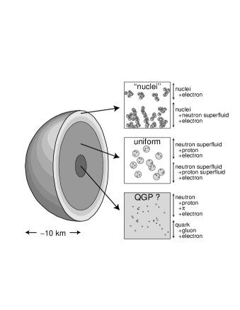
Figure 1: Schematic picture of a possible neutron star structure.

It has been claimed that usual MC satisfies only the first three conditions, and the final one is violated because it assumes the local charge neutrality in each phase instead of the global charge neutrality. A naive application of the Gibbs conditions to separate bulk phases without the surface and the Coulomb interaction, demonstrates a broad density-region of the structured mixed phase [1, 6]. When one takes into account the geometrical structures like droplet, rod and slab by extending the bulk calculation, one can see that the surface tension and Coulomb interaction determine their size [17, 2, 3]. However, the charge screening effect (caused by the rearrangement of the charged-particle distributions) should be very important when the typical size is of the order of the minimal Debye screening length in the problem. It may largely affect the stability condition of the geometrical structures in the mixed phases. We have been recently exploring the effect of the charge screening in the context of the various structured mixed phases [3, 4, 12, 27].

Our aim here is to investigate the non-uniform structures in nuclear matter numerically by means of the density functional theory with a relativistic mean field (RMF) model. Our framework allows one to determine the density profiles exactly without any sharp boundary and the surface tension used in the bulk calculations. It includes the Coulomb interaction in a proper way and we can fully take into account the charge screening effects. We shall figure out how the charge screening effects induce the rearrangement of the charged-particle distributions and thereby modify the results obtained by the bulk calculations.

2 Nuclear pastas

First we consider the nuclear pastas. At subnuclear densities, where pressure of the uniform nuclear matter is negative, so called “nuclear pastas” may appear [17]. In view of the phase transition, these can be regarded as the mixed phases following the liquid-gas phase transition in nuclear matter. Stable nuclear shape may change from sphere to rod, slab, tube and to bubble with increase of the matter density. Pastas are eventually dissolved into the uniform matter (liquid phase) at a certain nucleon density below the saturation density, $\rho_{0}\simeq 0.16~{}$fm^-3.

Existence of such pasta phases instead of the crystalline lattice of nuclei or the liquid $npe$ phase would modify some important processes by changing the hydrodynamic properties and the neutrino opacity in the supernova matter and in the protoneutron stars. Also the pasta phases may influence neutron star quakes and pulsar glitches via the change of mechanical properties of the crust matter.

A number of authors have discussed the nuclear pastas using various models [17, 18, 19, 20, 21, 22, 23, 24, 25], but most of them have relied on the bulk calculations; roughly speaking, the favorable nuclear shape is determined by a balance between the surface and the Coulomb energies. Thus the Coulomb interaction as well as the surface tension has an crucial role in the non-uniform pasta structures. However, the treatment of the Coulomb interaction so far has been rather simple and the rearrangement effect on the density profiles of the charged particles by the Coulomb interaction has been discarded in the bulk calculations. The paper [26] discusses the effect of electron screening to demonstrate that it is of a minor importance, but the rearrangement of the proton density as a consequence of the Coulomb repulsion was not shown up in their study.

2.1 Density functional theory with relativistic mean field

Following the idea of the density functional theory (DFT) with the RMF model [28], we can formulate equations of motion to study non-uniform nuclear matter numerically. The RMF model with fields of mesons and baryons introduced in a Lorentz-invariant way is simple for numerical calculations, but realistic enough to reproduce the bulk properties of finite nuclei as well as saturation properties in nuclear matter. In our framework, the Coulomb interaction is properly included in equations of motion for nucleons, electrons, and meson mean-fields, and we solve the Poisson equation for the Coulomb potential $V_{\rm Coul}$ self-consistently with them. Thus the baryon and electron density profiles, as well as the meson mean-fields, are determined in a way fully consistent with the Coulomb potential.

To begin with, we present the thermodynamic potential for the neutron, proton and electron system with chemical potentials $\mu_{n}$, $\mu_{p}$ and $\mu_{e}$, respectively;

$$\Omega=\Omega_{N}+\Omega_{M}+\Omega_{e},$$ (2)

where

$$\Omega_{N}=\sum_{a=p,n}\int d^{3}r\left[\int_{0}^{k_{{\rm F},a}}{d^{3}k\over 4\pi^{3}}\sqrt{{m_{N}^{*}}^{2}+k^{2}}-\rho_{a}\nu_{a}\right],$$ (3)

with the local Fermi momenta, $k_{{\rm F},a}({\bf r})(a=n,p)$, for nucleons,

$$\Omega_{M}=\int d^{3}r\left[{(\nabla\sigma)^{2}+m_{\sigma}^{2}\sigma^{2}\over 2}+U(\sigma)-{(\nabla\omega_{0})^{2}+m_{\omega}^{2}\omega_{0}^{2}\over 2}-{(\nabla R_{0})^{2}+m_{\rho}^{2}R_{0}^{2}\over 2}\right],$$ (4)

for the scalar ($\sigma$) and vector mean-fields ($\omega_{0},R_{0}$) and

$$\Omega_{e}=\int d^{3}r\left[-{1\over 8\pi e^{2}}(\nabla{V_{\rm Coul}})^{2}-{(\mu_{e}-{V_{\rm Coul}})^{4}\over 12\pi^{2}}\right],$$ (5)

for electrons and the Coulomb potential, $V_{\rm Coul}({\bf r})$, where $\nu_{p}({\bf r})=\mu_{p}+{V_{\rm Coul}({\bf r})}-g_{\omega N}\omega_{0}({\bf r})-g_{\rho N}R_{0}({\bf r}),\ \ \nu_{n}({\bf r})=\mu_{n}-g_{\omega N}\omega_{0}({\bf r})+g_{\rho N}R_{0}({\bf r}),\ \ m_{N}^{*}({\bf r})=m_{N}-g_{\sigma N}\sigma({\bf r})$, and the nonlinear potential for the scalar field, $U(\sigma)={1\over 3}bm_{N}(g_{\sigma N}\sigma)^{3}+{1\over 4}c(g_{\sigma N}\sigma)^{4}$. Temperature $T$ is kept to be zero in the present study.

Here we used the local-density approximation (LDA) for nucleons and electrons. Strictly speaking, LDA is meaningful only if the typical length of the nucleon density variation is larger than the inter-nucleon distance. To go beyond LDA we must take into account some derivative terms with respect to particle densities, which can be easily incorporated in the quasi-classical manner by the derivative expansion within the density functional theory [28]. In the case when we suppress derivative terms of nucleon densities they follow changes of the meson mean fields and the Coulomb field that have derivative terms. We must also bear in mind that for small structure sizes, quantum effects become prominent which we disregarded. Here we consider large-size pasta structures and simply discard the derivative terms, as a first-step calculation.

Parameters of the RMF model are chosen to reproduce saturation properties of nuclear matter: the minimum energy per baryon $-16.3$ MeV at $\rho=\rho_{0}=0.153$ fm^-3, the incompressibility $K(\rho_{0})=240$ MeV, the effective nucleon mass $m_{N}^{*}(\rho_{0})=0.78m_{N}$; $m_{N}=938$ MeV, and the isospin-asymmetry coefficient $a_{\rm sym}=32.5$  MeV. Coupling constants and meson masses used in our calculation are listed in Table 1.

Table 1: Parameter set used in RMF in our calculation.

$g_{\sigma N}$	$g_{\omega N}$	$g_{\rho N}$	$b$	$c$	$m_{\sigma}$ [MeV]	$m_{\omega}$ [MeV]	$m_{\rho}$ [MeV]
6.3935	8.7207	4.2696	0.008659	0.002421	400	783	769

From the variational principle ${\delta\Omega\over\delta\phi_{i}({\bf r})}=0$ ($\phi_{i}=\sigma,R_{0},\omega_{0},V_{\rm Coul}$) and ${\delta\Omega\over\delta\rho_{a}({\bf r})}=0$ ($a=n,p,e$), we get the coupled equations of motion for the mean-fields and the Coulomb potential,

$$\nabla^{2}\sigma({\bf r}) = m_{\sigma}^{2}\sigma({\bf r})+{dU\over d\sigma}-g_{\sigma N}(\rho_{n}^{(s)}({\bf r})+\rho_{p}^{(s)}({\bf r})),$$ (6)

$$\nabla^{2}\omega_{0}({\bf r}) = m_{\omega}^{2}\omega_{0}({\bf r})-g_{\omega N}(\rho_{p}({\bf r})+\rho_{n}({\bf r})),$$ (7)

$$\nabla^{2}R_{0}({\bf r}) = m_{\rho}^{2}R_{0}({\bf r})-g_{\rho N}(\rho_{p}({\bf r})-\rho_{n}({\bf r})),$$ (8)

$$\nabla^{2}{V_{\rm Coul}({\bf r})} = 4\pi e^{2}{\rho_{\rm ch}({\bf r})},$$ (9)

with the scalar densities $\rho_{a}^{(s)}({\bf r}),a=n,p$, and the charge density, ${\rho_{\rm ch}({\bf r})}={\rho_{p}({\bf r})}+{\rho_{e}({\bf r})}$. Equations of motion for fermions yield the standard relations between the densities and chemical potentials,

$$\mu_{n} = \sqrt{k_{{\rm F},n}^{2}({\bf r})+{m_{N}^{*}({\bf r})}^{2}}+g_{\omega N}\omega_{0}({\bf r})-g_{\rho N}R_{0}({\bf r}),$$ (10)

$$\mu_{p} = \mu_{n}-\mu_{e}=\sqrt{k_{{\rm F},p}^{2}({\bf r})+{m_{N}^{*}({\bf r})}^{2}}+g_{\omega N}\omega_{0}({\bf r})+g_{\rho N}R_{0}({\bf r})-{V_{\rm Coul}({\bf r})},$$ (11)

$${\rho_{e}({\bf r})} = -(\mu_{e}-{V_{\rm Coul}({\bf r})})^{3}/3\pi^{2},$$ (12)

where we have assumed the chemical equilibrium among nucleons and electrons. The baryon-number chemical potential $\mu_{B}$ equals to $\mu_{n}$ and the charge chemical potential $\mu_{Q}$ to $\mu_{e}$. Note that first, the Poisson equation for the Coulomb field (9) is a highly nonlinear equation in $V_{\rm Coul}({\bf r})$, since $\rho_{\rm ch}({\bf r})$ in r.h.s. includes it in a complicated way. Secondly, the Coulomb potential always enters equations through the gauge invariant combinations $\mu_{e}-V_{\rm Coul}({\bf r})$ and $\mu_{p}+V_{\rm Coul}({\bf r})$. Thirdly, solutions of these equations of motion attain the kinematical equilibrium, i.e. equal pressure in each spatial point, which is one of the Gibbs conditions.

2.2 Numerical procedure

To solve the above coupled equations numerically, we use the Wigner-Seitz cell approximation: the whole space is divided into equivalent cells with a geometry. The geometrical shape of the cell changes: sphere in three dimensional (3D) calculation, cylinder in 2D and slab in 1D, respectively. Each cell is globally charge-neutral and all the physical quantities in a cell are smoothly connected to those of the next cell with zero gradients at the boundary. Every point inside the cell is represented by the grid points (number of grids $N_{\rm grid}\approx 100$) and the differential equations for fields are solved by the relaxation method under the constraints of the given baryon number and the global charge neutrality.

To illustrate how to solve equations of motion for mean-fields, let us consider, for simplicity, two fields $f_{1}(r)$, $f_{2}(r)$ and their coupled Poisson-like equations under 3D calculation,

$$\nabla^{2}f_{1}(r) = {m_{1}}^{2}f_{1}(r)+W_{1}[f_{1},f_{2}],$$

$$\nabla^{2}f_{2}(r) = {m_{2}}^{2}f_{2}(r)+W_{2}[f_{1},f_{2}],$$ (13)

where $W_{i}(i=1,2)$ are functions of the fields $f_{1}$ and $f_{2}$. Introducing a relaxation “time” $t$ we solve

$${df_{i}(r)\over dt} = c_{i}\left(\nabla^{2}f_{i}(r)-{m_{i}}^{2}f_{i}(r)-W_{i}\right).$$ (14)

If coefficients $c_{i}$ are appropriately chosen, the above $f_{i}$ will converge in time and we get the solution of Eq. (13).

Baryon densities are solved with the help of the “local chemical potentials” $\mu_{a}(r)$ ($a=n,p$), being different from the above introduced constant chemical potentials. Assuming $\mu_{n}(r)$ being an increasing function of the neutron density $\rho_{n}(r)$ in Eq. (10), the relaxation equation for the neutron density,

$${d\rho_{n}(r)\over dt} = c_{n}(r)\;\rho_{n}(r)\nabla^{2}\mu_{n}(r),$$ (15)

is solved to equalize the local chemical potential $\mu_{n}(r)$ in each point. The coefficient $c_{n}(r)$ is chosen to conserve the total neutron number. The proton density $\rho_{p}(r)$ is adjusted in the same way. When we impose the beta-equilibrium condition, proton and neutron densities are adjusted to achieve $\mu_{n}(r)=\mu_{p}(r)+\mu_{e}(r)$. Finally we get densities $\rho_{n}(r)$ and $\rho_{p}(r)$ leading the constant chemical potentials $\mu_{n}(r)=\mu_{n}$ and $\mu_{p}(r)=\mu_{p}$. Nevertheless, the basic idea is to obtain constant chemical potentials, $\mu_{a}(r)=\mu_{a}(a=n,p)$ at the convergence. There is an exception: when there are some regions where $\rho_{a}(r)=0$, the local chemical potential $\mu_{a}(r)$ is larger than the corresponding constant value in the regions with finite $\rho_{a}(r)$.

The electron density $\rho_{e}(r)$ is calculated directly from Eq. (12). The value of $\mu_{e}$ is adjusted at any time step to get global charge neutrality: we decrease $\mu_{e}$ when total charge in a cell is positive and increase when it is negative.

All the above relaxation procedures are performed simultaneously, which means that our numerical procedure always respect the Gibbs conditions for chemical potentials.

3 Bulk properties of finite nuclei

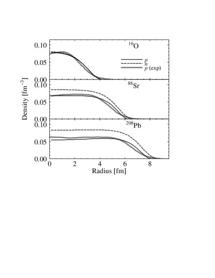
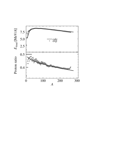
Figure 2: Left: the density profiles of typical nuclei. The proton densities (solid curves) are compared with the experiment. Right: binding energy per nucleon and the proton ratio of finite nuclei.

Before applying our framework to the problem of the nuclear pastas , we check how it works to describe the bulk properties of finite nuclei. In this calculation for simplicity we assume the spherical shape of nucleus. The electron density is set to be zero. Therefore the global charge neutrality condition is not imposed.

In Fig. 2 (left panel) we show the density profiles of some typical nuclei. One can see how well our framework may reproduce density profiles. To get a better fit, especially near the surface, we could include the derivative terms of the nucleon densities, as we have mentioned. Fine structures seen in the empirical density profiles, which come from the shell effects (see, e.g., a proton density dip at the center of a light ¹⁶O nucleus), cannot be reproduced by the mean-field approach. The effect of the rearrangement of the proton density can be seen in heavy nuclei; protons repel each other that enhances their concentration near the surface of the heavy nuclei. This effect is analogous to the charge screening effect in a sense that the proton distribution is now changed not on the scale of the radius of the nucleus, as for bare Coulomb field, but on another length scale, that we will call the proton Debye screening length, see Eq. (17) below. It has important consequences for the pasta structures since typically the proton Debye length is less than the droplet size. The stable value of the proton fraction $Y_{p}=Z/A$ ($Z$ and $A$ are proton and total baryon numbers, respectively) is obtained by imposing the beta equilibrium condition $\mu_{n}=\mu_{p}$ for a given baryon number. Figure 2 (right panel) shows the baryon number dependencies of the binding energy per baryon and the proton ratio. We can see that the bulk properties of finite nuclei (density, binding energy, and proton to baryon ratio) are satisfactorily reproduced for our present purpose.

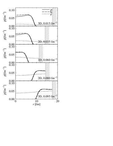
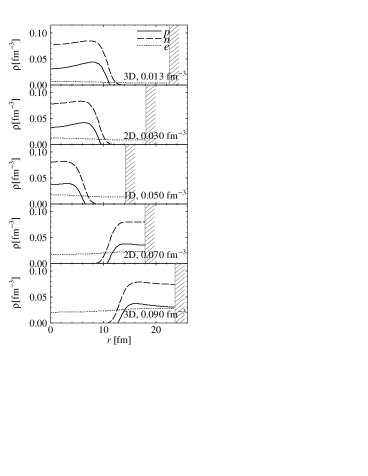
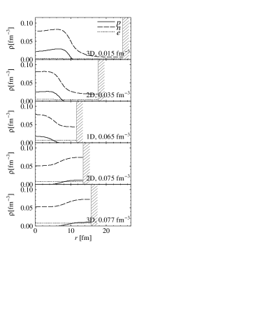
Figure 3: Examples of the density profiles in the cell for symmetric nuclear matter with $Y_{p}$=0.5 (left) and for asymmetric matter with $Y_{p}=0.3$ (center) and 0.1 (right).

Note that we must use a slightly smaller value of the sigma mass i.e. 400 MeV, than that one usually uses to get an appropriate fit. If we used a popular value $m_{\sigma}\approx 500$ MeV, finite nuclei would be overbound by about 3 MeV/$A$. The actual value of the sigma mass (as well as the omega and rho masses) has little relevance for the case of infinite nuclear matter, since it enters the thermodynamic potential only in the combination $\widetilde{C}_{\sigma}=g_{\sigma N}/m_{\sigma}$. However meson masses are important characteristics of finite nuclei and of other non-uniform nucleon systems, like those in pastas. The effective meson mass characterizes the typical scale for the spatial change of the meson field and consequently it affects, e.g., the surface property of the given nucleon structure and it influences the value of the effective surface tension.

4 Non-uniform structures in nuclear matter

4.1 Nucleon matter at fixed proton fraction

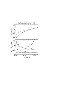
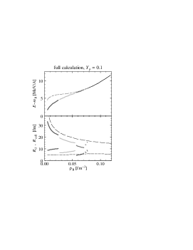
Figure 4: Binding energies per nucleon and the cell size for symmetric nuclear matter with $Y_{p}$=0.5 (left), and for asymmetric matter with $Y_{p}=0.3$ (middle) and 0.1 (right).

First, we focus on the discussion of the behavior of the nuclear matter at a fixed proton fraction $Y_{p}$. Particularly, we explore proton fractions $Y_{p}=0.1$, 0.3, and 0.5. The cases $Y_{p}=0.3$ – 0.5 might be relevant for the supernova matter and for newly born neutron stars. Figure 3 shows some density profiles inside the Wigner-Seitz cells as functions of the radial distance from the center of the cell. The geometrical dimension of the cell is denoted as “3D” (three dimensional), etc. The cell boundary is indicated by the hatch. From the top to the bottom the configuration changes like droplet (3D), rod (2D), slab (1D), tube (2D), and bubble (3D). Thus the nuclear pastas are clearly manifested. For the lowest $Y_{p}$ case ($Y_{p}=0.1$), the neutron density is finite at any point: the space is filled by dripped neutrons. For a higher $Y_{p}$, the neutron density drops to zero outside the structure. The proton density always drops to zero outside the nuclear lump. The charge screening effects are pronounced, especially due to protons. Protons repel each other and thereby the proton density profile substantially deviates from the step-function: the proton number is enhanced near the surface of the nuclear lump. The electron density also becomes non-uniform by the rearrangement effect. This non-uniformity of the electron distribution is more pronounced for a higher $Y_{p}$ and a higher density.

EOS of the nuclear pastas is shown as a function of the averaged density in Fig. 4 (upper panels). The energy $E-m_{B}$ includes the kinetic energy of electrons, which makes the total pressure positive. The lowest-energy configuration is selected among various geometrical structures for a given averaged density. The most favorable configuration changes from the droplet to rod, slab, tube, bubble, and to the uniform one (the dotted thin curve) with increase of the density. We can see that the appearance of the nuclear pastas results in a softening of the EOS: the energy per baryon gets lower up to about 15 MeV$/A$ compared to the uniform case. The lower panels in Fig. 4 show the cell sizes $R_{\rm cell}$ and structure sizes $R_{\rm d}$ as functions of the averaged density. The size $R_{\rm d}$ is defined here by way of a density fluctuation as

$$R_{\rm d} = \cases{\displaystyle R_{\rm cell}{\langle\rho_{p}\rangle^{2}\over\langle\rho_{p}^{2}\rangle},\ \ \ \hbox{(for droplet, rod, and slab)}\cr\displaystyle R_{\rm cell}\left(1-{\langle\rho_{p}\rangle^{2}\over\langle\rho_{p}^{2}\rangle}\right),\ \ \ \hbox{(for tube and bubble)}}$$ (16)

where the bracket “$\langle\rangle$” indicates the average inside the cell. Dashed curves show the Debye screening lengths of electron and proton calculated as

$$\lambda^{(e)}_{D}=\left(-4\pi e^{2}{d\rho_{e}^{\rm av}\over d\mu_{e}}\right)^{-1/2},~{}~{}~{}\lambda^{(p)}_{D}=\left(4\pi e^{2}{d\rho_{p}^{\rm av}\over d\mu_{p}}\right)^{-1/2},$$ (17)

respectively, where $\rho_{p}^{\rm av}$ is the proton density averaged over the nuclear lump and $\rho_{e}^{\rm av}$ is the electron density averaged inside the cell. Note that these quantities are obviously gauge invariant. Numerically, the cell size $R_{\rm cell}$ for droplet, rod, and slab configurations at $Y_{p}=0.5$ and 0.3 are shown to be close to the Debye screening length of electron. For $Y_{p}=0.1$, in all cases $R_{\rm cell}$ is substantially smaller than $\lambda^{(e)}_{D}$ and thereby the electron screening should be much weaker. In all cases, except for bubbles (at $Y_{p}=0.5$ and 0.3), the structure size $R_{d}$ are smaller than $\lambda^{(e)}_{D}$. This means that the Debye screening effect of electrons inside these structures should not be pronounced. For bubbles at $Y_{p}=0.5$ and 0.3, $\lambda_{D}^{(e)}$ is substantially smaller than the cell size and the electron screening should be significant. For $Y_{p}=0.5,0.3,0.1$ in all cases (with the only exception $Y_{p}=0.1$ for slabs), the value $\lambda_{D}^{(p)}$ is shorter than $R_{\rm d}$, which means that the rearrangement of proton density is essential for the structures of the nuclear pastas, as it is indeed seen from the Fig. 3.

   Problem: Evaluate the electron Debye screening length in the case of $\rho_{e}^{\rm av}=-0.5\rho_{0}$, by using the above expression Eq. (17) for massless electrons.   

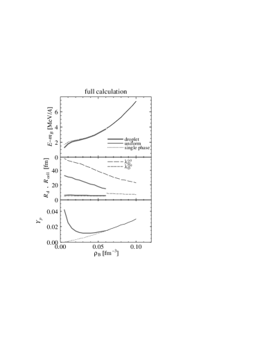
Figure 5: Binding energy (top), structure size (middle), and proton ratio (bottom) in the cell for nuclear matter in beta equilibrium.

Using the baryon density and the structure size from Fig. 4, one may estimate the atomic number of the structure. In the case of droplets and for $Y_{p}=0.5$ the atomic number of the droplet is $\simeq 25$ at lower density limit and $\simeq 65$ at the maximum density of the droplet phase $\rho_{B,d}^{(\rm max)}\simeq 0.025\ {\rm fm}^{-3}$.

4.2 Nuclear matter in beta equilibrium

Next, we explore the nuclear pastas in beta equilibrium. The droplet structure appears, which is quite similar to the above considered case of the fixed proton ratio $Y_{p}=0.1$. The apparently different feature in this case is that only the droplet configuration appears as a non-uniform structure. It should be noticed, however, that the presence or absence of the each pasta structure may sensitively depend on the choice of the effective interaction.

In Fig. 5 we plot EOS (top), the structure size (middle), and the proton ratio (bottom). The difference between EOS of uniform matter and that of non-uniform one is small, while the proton ratio is significantly affected by the presence of the pasta at lower densities. The droplet radius and the cell radius in the middle panel of Fig. 5 are always smaller than the electron Debye length $\lambda_{D}^{(e)}$, and thereby the effect of the electron charge screening is small. On the other hand, the proton Debye length $\lambda_{D}^{(p)}$ is comparable with the droplet radius at all densities, which demonstrates the relevance of the proton screening.

5 Charge screening effect in nuclear pastas

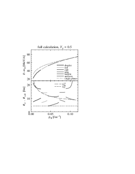
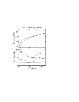
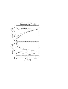
Figure 6: Comparison of the density profiles for different treatments of the Coulomb interaction. From the left: “full” calculation, “no Coulomb” calculation, and “bulk” calculation. The proton ratio for all cases is $Y_{p}$=0.5.

In this section we explore the effect of the charge screening on the nuclear pastas. Here we focus on the matter with fixed proton ratio $Y_{p}=0.5$ since the Coulomb effects should be most pronounced in this case. We compare three kinds of calculations with different treatments of the Coulomb interaction. One is the “full calculation” which we have presented above. The second calculation (“no Coulomb”) is performed by totally discarding the Coulomb potential $V_{\rm Coul}$ in equations of motion. After getting the density profiles, the Coulomb energy, being evaluated using charge densities thus determined, is added to the total energy. Note that this calculation is similar but not the same as the bulk calculations: in the latter a sharp boundary and the surface tension are introduced, and the particle density profile is assumed to be constant in each phase. The third is the bulk calculation, in which we use a completely uniform electron density, the baryon density distribution of a step function, and the surface tension introduced by hand. To determine the geometrical structure we have used the equilibrium condition of baryon chemical potential and the pressure calculated the present RMF model, and the relation between surface energy $E_{\rm surf}$ and the Coulomb energy $E_{\rm Coul}$ [17] as

$$E_{\rm surf} = 2E_{\rm Coul}.$$ (18)

We have used the surface tension parameter $\tau=1.03$ MeV/fm² to fit the liquid-drop binding energies of finite nuclei.

EOS as a whole (upper panels in Fig. 6) shows almost no dependence on the calculation. This agrees with a general statement that the variational functional is always less sensitive to the choice of the trial functions than the quantities depending on these trial functions linearly.

Nevertheless, the density region of pasta structures and the sizes of the structures (lower panels in Fig. 6) especially for tube and bubbles are different. In fact we don’t observe tube and bubble configurations in the present bulk calculation. In Ref. [17] and others, however, they have reported the appearance of full pasta structures by the bulk calculation. The most important origin of this discrepancy may come from the difference in the nuclear EOS used in the calculation. Also the surface tension is crucial; if we use smaller value of $\tau$, e.g. 0.3 MeV/fm², we observe full pasta structures appear in wider density range. If we take $\tau=0$ the mixed phase spreads from zero to the saturation density $\rho_{0}$ without any specific geometry. From the bulk calculation we see that the surface tension plays a crucial role in the appearance of pasta structures.

Comparing the “no Coulomb” calculation with “full calculation”, we don’t see large difference. However, precisely looking, the density region of pasta in “full calculation” is slightly larger. The density dependence of the cell size is also different. In the case of “no Coulomb” all the pieces of lines for $R_{\rm cell}$ are monotonously decreasing. The behavior of $R_{\rm cell}$ in the full calculation is rather similar to the bulk calculation.

6 Kaon condensation in high-density matter

Figure 7: Onset mechanism of kaon condensation.

Figure 8: Original EOS and the Maxwell construction.

Next we explore the high-density nuclear matter in beta-equilibrium, which is expected to exist in the inner core of neutron stars. Kaons are the lightest mesons with strangeness, and their effective energy is much reduced by the kaon-nucleon interaction in nuclear medium. For low-energy kaons the $s$-wave interaction is dominant and attractive in the $I=1$ channel, so that negatively charged kaons appear in the neutron-rich matter once the process $n\rightarrow p+K^{-}$ becomes energetically allowed. Since kaons are bosons, it causes the Bose-Einstein condensation at momentum ${\bf p}=0$ [29]. The threshold condition then reads

$$\epsilon_{-}({\bf p}=0)=\mu_{n}-\mu_{p}=\mu_{e},$$ (19)

which means the kaon distribution function diverges at ${\bf p}=0$ (Fig. 8).

If kaon condensation occurs in nuclear matter, it has many implications on compact stars; softening of EOS may give the possibility of the delayed collapse of a supernova to the low-mass black hole, and the nucleon Urca process under background kaons may give a fast cooling mechanism of neutron stars [30, 31, 32, 33, 34].

Since many studies have shown that kaon condensation is of the first order, we must carefully treat the phase change (Fig. 8). In the following we discuss the kaon mixed phase in a similar way to nuclear pastas. There have been some studies about the mixed phase in the kaon condensation [5, 6, 7, 8, 9, 10, 11, 12]. In ref.[11] the charge screening effect has been also studied, but all the equations of motion have not been solved self-consistently.

Table 2: Additional parameters used in RMF with kaon. The kaon optical $U_{K}$ is defined by $U_{K}=g_{\sigma K}\sigma+g_{\omega K}\Omega_{0}$.

$f_{K}(\approx f_{\pi})$ [MeV]	$m_{K}$ [MeV]	$g_{\omega K}$	$g_{\rho K}$	$U_{K}(\rho_{0})$ [MeV]
93	494	$g_{\omega N}/3$	$g_{\rho N}$	$-120$ – $-130$

To incorporate kaons into our calculation, the thermodynamic potential of Eq. (2) is modified as

$$\Omega = \Omega_{N}+\Omega_{M}+\Omega_{e}+\Omega_{K},$$ (20)

$$\Omega_{K} = \!\!\!\int d^{3}r\left[-{f_{K}^{2}\theta^{2}\over 2}\left[-{m_{K}^{*}}^{2}+(\mu_{K}-V_{\rm Coul}+g_{\omega K}\omega_{0}+g_{\rho K}R_{0})^{2}\right]+{f_{K}^{2}(\nabla\theta)^{2}\over 2}\right],$$ (21)

where $m_{K}^{*}=m_{K}-g_{\sigma K}\sigma$,  $\mu_{K}=\mu_{e},$  and the kaon field $K=f_{K}\theta/\sqrt{2}$ ($f_{K}$ : Kaon decay constant). The equations of motion are then similar to Eqs. (5) - (11) given for nuclear pastas except kaon contributions [12]. Additional parameters concerning kaons are presented in Table 2.

If Glendenning’s claim were correct, the structured mixed phase would develop in a broad density range from well below to well above the critical density [5, 6, 7]. In this density interval the matter should exhibit the structure change similar to the nuclear pastas [27]: the kaonic droplet, rod, slab, tube, bubble. Actually we observe such structures (kaonic pastas) in our calculation. In the top (a) and the middle (b) panels of Fig. 9 we show EOS; pieces of solid curves indicate the energetically most favored structures, while the dotted curve EOS of the uniform matter. One can see the softening of EOS by the appearance of kaonic pastas. In the bottom panel (c) plotted are the size of the kaonic lump or hole and the cell size.

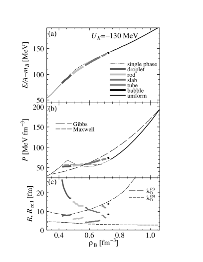
Figure 9: Top: binding energy per nucleon of nuclear matter in beta equilibrium. Middle: pressure. Bottom: structure size $R$ (thick curves below) and the cell size $R_{\rm cell}$ (thick curves above).

The dashed lines show the Debye screening lengths of the electron and the proton, $\lambda_{D}^{(e)}$ and $\lambda_{D}^{(p)}$, respectively. In most cases $\lambda_{D}^{(e)}$ is less than the cell size $R_{\rm cell}$ but it is larger than the structure size $R$. However the proton Debye length $\lambda_{D}^{(p)}$ is always shorter than $R_{\rm cell}$ and $R$. When the minimal value of the Debye length inside the structure is shorter or of the order of $R$, the charge screening effects should be pronounced [3].

7 Charge screening effect in the kaon mixed phase

To demonstrate the charge screening effect on the kaonic mixed phase and discuss differences among various treatments , we show pressure $P$ ($=-\Omega/V$) in the middle panel (b) of Fig. 9 and the phase diagrams in the $\mu_{B}$-$\mu_{e}$ plane in Fig. 10. From Fig. 9 (b) we can clearly see that our results give the similar pressure to the one given by MC, while the bulk calculation, where no Coulomb interaction or surface energy is taken into account, gives a wide density region for the mixed phase.

We can get more insight about the role of the Coulomb interaction in Fig. 10; left panel in Fig. 10 exhibits the full calculation, while in the right panel we show the case, when the electric potential is discarded in determining the density profile (“No Coulomb”) and the Coulomb energy, using the density profile thus determined, is then added to the total energy. We use “No Coulomb” in the same meaning as in the nuclear pastas. We see that in “No Coulomb” case the pieces of solid curves lie between two curves given by the bulk calculation (indicated by “Gibbs”), where the Gibbs conditions are imposed disregarding the surface tension and the Coulomb interaction, and by the Maxwell construction (indicated by “Maxwell”). The “Full calculation” case is more close to the one given by the Maxwell construction. As follows from the density profiles shown in Fig. 11, the local charge neutrality is more pronounced in the case of the “Full calculation” (smaller difference of kaon and proton densities). These results suggest that the Maxwell construction is effectively meaningful owing to the charge screening effects.

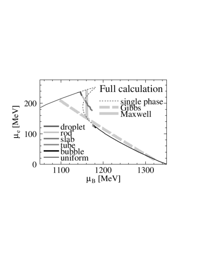
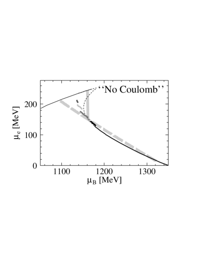
Figure 10: Phase diagram in the $\mu_{B}$-$\mu_{e}$ plane, where $\mu_{B}$ and $\mu_{e}$ denote baryon- and charge-chemical potentials, respectively. Left: full calculation. Right: the electric potential is discarded in determining the matter structure. Curves calculated using Gibbs conditions disregarding finite size effects and the Coulomb interaction effect (“Gibbs”) and that for the Maxwell construction (“Maxwell”) are also presented for comparison.

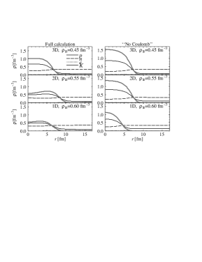
Figure 11: Comparison of density profiles of kaonic matter calculated with and without the Coulomb interaction. The cell size is not optimized in this comparison.

8 Summary and concluding remarks

We have discussed two kinds of the non-uniform structures in nuclear matter, nuclear pastas at subnuclear densities and the kaon mixed phase above the nuclear density, which may arise as consequences of FOPT with many particle species, and elucidated the charge screening effect. Using a self-consistent framework based on density functional theory and relativistic mean fields, we took into account the Coulomb interaction in a proper way and numerically solved coupled equations of motion to extract the density profiles of nucleons, electrons and kaons.

First of all, we have checked how realistic our framework is by studying the bulk properties of finite nuclei, as well as the saturation properties of nuclear matter, and found that it can describe both features satisfactorily. One could still improve the consideration by including the gradient terms of the nucleon densities, which may give a better description of the nuclear surface.

In isospin-asymmetric nuclear matter with fixed proton to atomic number ratios, we have observed the “nuclear pastas” with various geometrical structures at sub-nuclear densities. These cases are relevant for the discussion of the supernova explosions and for the description of the newly born neutron stars. The appearance of the pasta structures significantly lowers the energy, i.e. softens the equation of state, while the energy differences between various geometrical structures are rather small.

By comparing different treatments of the Coulomb interaction, we have seen that the self-consistent inclusion of the Coulomb interaction changes the phase diagram. In particular the region of pasta structure is broader for “full” calculation compared to that with simplified treatments of the Coulomb interaction which have been used in the previous studies. The effect of the rearrangement of the proton distributions on the structures is much more pronounced compared to the effect of the electron charge screening. The influence of the charge screening on the equation of state, on the other hand, was found to be small.

We have also studied the structure of the nucleon matter in the beta equilibrium. We have found that only one type of structures is realized: proton-enriched droplets embedded in the neutron sea. No other geometrical structures like rod, slab, etc. appeared.

We have discussed how the geometrical structures manifest in the context of kaon condensation. Our framework can be extended to include kaons straightforwardly. We have discussed the effect of the charge screening in this case. Since the kaon mixed-phase appear at high-densities, we see that changes are more remarkable than for the “nuclear pastas” at subnuclear densities [27]. The density range of the structured mixed phase is largely limited by the charge screening and thereby the phase diagram becomes similar to that given by the Maxwell construction. Although the importance of such a treatment has been demonstrated for the hadron-quark matter transition [3, 4], one of our new findings here is that we can figure out the role of the charge screening effect without introducing an “artificial” input of the surface tension. In our study we have used the one-boson-exchange interaction for the $KN$ interaction. On the other hand the bulk calculation, where no Coulomb interaction nor surface tension is included, can not give the mixed phase in the chiral model [8, 9]. It should be interesting to study the effects of the charge screening to see whether the chiral model is not thermodynamically well-defined.

In application to the newly formed neutron stars like in supernova explosions, finite temperature and neutrino trapping effects become important, as well as the dynamics of the first order phase transition with formation of the structures. It would be interesting to extend our framework to include these effects.

References

- [1] N. K. Glendenning, Phys. Rev. D46 1274 (1992); N. K. Glendenning, Phys. Rep. 342 393 (2001).
- [2] H. Heiselberg, C. J. Pethick and E. F. Staubo, Phys. Rev. Lett. 70 1355 (1993).
- [3] D. N. Voskresensky, M. Yasuhira and T. Tatsumi, Phys. Lett. B541, 93 (2002); Nucl. Phys. A723 291 (2003); T. Tatsumi and D. N. Voskresensky, nucl-th/0312114.
- [4] T. Endo, Toshiki Maruyama, S. Chiba and T. Tatsumi, nucl-th/0410102; in this volume.
- [5] N. K. Glendenning and J. Schaffner-Bielich, Phys. Rev. C60 025803 (1999).
- [6] M. Christiansen and N. K. Glendenning, astro-ph/0008207.
- [7] M. Christiansen, N. K. Glendenning and J. Schaffner-Bielich, Phys. Rev. C62 025804 (2000).
- [8] J. A. Pons, S. Reddy, P. J. Ellis, M. Prakash and J. M. Lattimer, Phys. Rev., C62 035803 (2000).
- [9] T. Tatsumi and M. Yasuhira, Nucl. Phys. A 653, 133 (1999); M. Yasuhira and T. Tatsumi, Nucl. Phys. A690 769 (2001).
- [10] S. Reddy, G. Bertsch and M. Prakash, Phys. Lett., B475 1 (2000).
- [11] T. Norsen and S. Reddy, Phys. Rev. C63 065804 (2001).
- [12] T. Maruyama, T. Tatsumi, V. N. Voskresensky, T. Tanigawa and S. Chiba, Nucl. Phys. A 749 (2005) 186c.
- [13] M. Alford, K. Rajagopal, S. Reddy and F. Wilczek, Phys. Rev. D64 074017 (2001).
- [14] P. F. Bedaque, Nucl. Phys. A697 569 (2002).
- [15] S. Reddy and G. Rupak, nucl-th/0405054.
- [16] P. F. Bedaque, H. Caldas and G. Rupak, Phys. Rev. Lett. 91 247002 (2003).
- [17] D. G. Ravenhall, C. J. Pethick and J. R. Wilson, Phys. Rev. Lett. 27, 2066 (1983).
- [18] M. Hashimoto, H. Seki and M. Yamada, Prog. Theor. Phys. 71, 320 (1984).
- [19] R. D. Williams and S. E. Koonin, Nucl. Phys. A435, 844 (1985).
- [20] K. Oyamatsu, Nucl. Phys. A561, 431 (1993).
- [21] C. P. Lorentz, D. G. Ravenhall and C. J. Pethick, Phys. Rev. Lett. 25, 379 (1993).
- [22] K. S. Cheng, C. C. Yao and Z. G. Dai, Phys. Rev. C55, 2092 (1997).
- [23] Toshiki Maruyama, K. Niita, K. Oyamatsu, Tomoyuki Maruyama, S. Chiba and A. Iwamoto, Phys. Rev. C57, 655 (1998); T. Kido, Toshiki Maruyama, K. Niita and S. Chiba, Nucl. Phys. A663-664, 877 (2000).
- [24] G. Watanabe, K. Iida and K. Sato, Nucl. Phys. A676, 445 (2000).
- [25] G. Watanabe, K. Sato, K. Yasuoka and T. Ebisuzaki, Phys. Rev. C66, 012801 (2002).
- [26] G. Watanabe and K. Iida, Phys. Rev. C68, 045801 (2003).
- [27] Toshiki Maruyama, T. Tatsumi, V. N. Voskresensky, T. Tanigawa, S. Chiba and Tomoyuki Maruyama, nucl-th/0402202.
- [28] Density Functional Theory, ed. E. K. U. Gross and R. M. Dreizler, Plenum Press (1995).
- [29] D.B. Kaplan and A.E. Nelson, Phys. Lett. B175, 57 (1986); B179, 409(E) (1986).
-
[30]
For review articles, T. Tatsumi, Prog. Theor. Phys. Suppl. 120, 111 (1995)
and references cited therein.
C.H. Lee, Phys. Rep. 275, 197 (1996).
M. Prakash, I. Bombaci, M. Prakash, P. J. Ellis, J. M. Lattimer, R. Knorren, Phys. Rep. 280, 1 (1997). - [31] G. E. Brown and H. A. Bethe, Astrophys. J. 423, 659 (1994).
- [32] G. E. Brown, K. Kubodera, D. Page and P. Pizzecherro, Phys. Rev.D37, 2042 (1988).
- [33] T. Tatsumi, Prog. Theor. Phys.80,22 (1988).
- [34] D. Page and E. Baron, Astrophys. J.254, L17 (1990).