Three-neutron resonance trajectories for realistic interaction models

Abstract

Three-neutron resonances are investigated using realistic nucleon-nucleon interaction models. The resonance pole trajectories are explored by first adding an additional interaction to artificially bind the three-neutron system and then gradually removing it. The pole positions for the three-neutron states up to $J$=5/2 are localized in the third energy quadrant – Im(E)$\leqslant 0$, Re(E)$\leqslant 0$ – well before the additional interaction is removed. Our study shows that realistic nucleon-nucleon interaction models exclude any possible experimental signature of three-neutron resonances.

I Introduction

The possible existence of pure neutron nuclei is a long standing ambiguity in nuclear physics. The neutron-neutron (nn) scattering length is negative and rather large $a_{nn}=-18.59\pm 0.40$ fm nn_scl4 , indicating that this system is almost bound in ${}^{1}\emph{S}_{0}$ state. This value is actually the signature of a virtual bound state just $\approx$100 keV above the threshold. It is thus expected that by adding a few neutrons, one can end up with a bound multineutron state, as it happens in some fermionic systems, like ³He atomic clusters Guardiola . This is the reason for the recurrent turmoils appearing in the nuclear physics society Oglobin ; Marques . However, the weakness of nuclear interaction in higher partial waves (namely P and D), in comparison with their centrifugal barriers, excludes the possibility of binding ’virtual’ dineutrons together Thesis . Recently, the non-existence of small bound multineutron clusters has been settled out theoretically Thesis ; Pieper ; Bertulani ; Natasha . Nevertheless, the existence of resonant states of such nuclei having observable effects had not yet been fully eliminated.

Indeed, in spite of numerous experimental and theoretical studies that exploit different reactions and methods, the situation concerning few-neutron resonances is not firmly established. One does not have clear ideas even for the simplest case: the three-neutron compound. A nice summary on the three-neutron system status up to 1987 can be found in 3N_analysis . A few more recent experimental studies have provided only controversial results. In He_3n_97 , the analysis of ${}^{3}He(\pi^{-},\pi^{+})3n$ process yielded no evidence of a three-neutron resonant state. The explanation 3n_res_exp_70 of double charge exchange differential cross sections in ³He in term of a broad ($E=2-6i$ MeV) three-neutron resonance were recently criticized by a more thorough experimental study 3n_res_exp_86 . Nevertheless the latter study further suggested the existence of a wide ³n resonance at even larger energies ($E\approx 20-20i$ MeV). Furthermore, very recent experimental results on ${}^{8}He(d,{{}^{6}Li})4n$ reaction have shown some discrepancies with what could be expected from phase space calculations, suggesting the existence of a resonant tetraneutron Exxon .

There exists several theoretical efforts to find ³n and ⁴n resonances. A variational study based on complex-scaling and simplified nucleon-nucleon (NN) interaction was carried out in Csoto with the prediction of a ³n resonance at $E=14-13i$ MeV for the $J^{\pi}=3/2^{+}$ state. On the other hand, no ³n nor ⁴n resonances were found by Sofianos et al. Sofianos using MT I-III potential; only the existence of some broad subthreshold ($E_{R}<0$) states was pointed out. Realistic NN forces can provide however different conclusions. These models contain interaction in P- and higher partial waves, which – due to the Pauli principle – are a crucial ingredient in binding fermionic systems. The only study performed using realistic potentials was carried by Glöckle and Witala 3n_res_gloe . These authors were not able to find any real three-neutron resonances. However due to some numerical instabilities, the full treatment of ³n system was not accomplished and the conclusions were drawn based on the phenomenological Gogny interaction Gogny . Reference Glockle_Hem is probably the most complete study of three neutron system. In this work, the trajectories for ³n states with $J\leqslant$3/2 have been traced by artificially enhancing a rank-2 separable nn interaction. Our work is devoted to complement the studies of references 3n_res_gloe ; Glockle_Hem . We have explored all ³n states up to $J$=5/2, fully relying on realistic NN interactions. Similarly to Ref. Glockle_Hem we have used two different methods, namely complex-scaling (CS) and analytical continuation in the coupling constant (ACCC), to trace the resonance trajectories. This allows us to check the reliability of our results, as well as to judge on the pertinence of the two methods used.

[Calculations presented in this paper use $\frac{\hbar^{2}}{m}=41.44$ MeV$\cdot$fm² as an imput for the mass of the neutrons.]

II Theoretical background

Resonance eigenfunctions correspond to complex energy solutions of the Schrödinger equation:

$$\widehat{H}\Psi_{res}=E_{res}\Psi_{res},\qquad E_{res}=\varepsilon_{res}-\frac{i}{2}\Gamma_{res}.$$ (1)

Since physical resonance have positive energy real parts, $\varepsilon_{res}>0$, the corresponding eigenfunctions are not square integrable. Nevertheless, by applying them a similarity transformation they can by mapped onto normalizable states. That is:

$$\left(\widehat{S}\widehat{H}\widehat{S}^{-1}\right)\left(\widehat{S}\Psi_{res}\right)=E_{res}\left(\widehat{S}\Psi_{res}\right)$$ (2)

with $\widehat{S}\Psi_{res}\rightarrow 0$ as $r\rightarrow\infty$.

Functions $\left(\widehat{S}\Psi_{res}\right)$ are in Hilbert space, although $\Psi_{res}$ are not. The complex-scaling method is defined by means of the similarity operator Moiseyev ; Ho :

$$\widehat{S}=e^{i\theta r\frac{\partial}{\partial r}},$$ (3)

such that any analytical function $f(r)$ is transformed according to:

$$\widehat{S}f(r)=f(re^{i\theta}).$$ (4)

For a broad class of potentials, complex-scaling operation does not affect the bound and resonant state spectra of the Hamiltonian $\widehat{H}$, provided $0\leqslant\theta<\frac{\pi}{2}$. However the continuous spectra of $\widehat{H}$ will be rotated by an angle $2\theta$. Resonance eigenfunctions $\left(\widehat{S}\Psi_{res}\right)$ of the scaled Hamiltonian become square integrable if  $2\theta>\left|\arg(E_{res})\right|$ and therefore the standard bound state techniques can be applied to determine the corresponding eigenvalues.

In order to solve the three-body problem we use Faddeev equations in configuration space Fadd_art , first derived by Noyes Fadd_art ; Noyes . Though this formalism was initially developed to investigate the three-body continuum, it turns to be very useful to treat bound-state problems as well. For three identical particles, the Faddeev-Noyes equations read:

$$\left(E-\widehat{H}_{0}-V_{ij}\right)\psi_{ij,k}=V_{ij}(P^{+}+P^{-})\psi_{ij,k}.$$ (5)

$\widehat{H}_{0}$ is the three-particle kinetic energy operator, $V_{ij}$ the two-body force, $\psi_{ij,k}$ the Faddeev component and $P^{+},P^{-}$ denotes cyclic particle permutation operators. The properly symmetrized three-body wave function is $\Psi=(1+P^{+}+P^{-})\psi_{ij,k}$. In order to simplify the kinetic energy operator and to separate internal and center of mass degrees of freedom we use Jacobi coordinates: $\overrightarrow{x_{ij}}=\overrightarrow{r_{j}}-\overrightarrow{r_{i}}$ and $\overrightarrow{y_{ij}}=\frac{2}{\sqrt{3}}\left[\overrightarrow{r_{k}}-\frac{1}{2}\left(\overrightarrow{r_{i}}+\overrightarrow{r_{j}}\right)\right]$.

Complex-scaling Faddeev equations causes no difficulties: one has simply to scale all the Jacobi vectors with the same exponential factor:

$$\overrightarrow{x_{ij}}\rightarrow\overrightarrow{x_{ij}}e^{i\theta}\qquad\text{and\qquad}\overrightarrow{y_{ij}}\rightarrow\overrightarrow{y_{ij}}e^{i\theta}.$$ (6)

Such transformation affects only the hyperradius $\rho=\sqrt{x_{ij}^{2}+y_{ij}^{2}}$, whereas neither the expressions of permutation operators – $P^{+},P^{-}$ – nor the angular dependence of Faddeev equations are affected. Using Jacobi coordinates, the kinetic energy operator can be expressed as a six-dimensional Laplacian $\widehat{H}_{0}=-\frac{\hbar^{2}}{m}\Delta_{\chi}$ with $\chi\equiv(\overrightarrow{x_{ij}},\overrightarrow{y_{ij}})$ and equation (5) transforms into:

$$\left[E+e^{-i2\theta}\Delta_{\chi}-V_{ij}\left(x_{ij}e^{i\theta}\right)\right]\widetilde{\psi}_{ij,k}(\overrightarrow{x_{ij}},\overrightarrow{y_{ij}})=V_{ij}\left(x_{ij}e^{i\theta}\right)(P^{+}+P^{-})\widetilde{\psi}_{ij,k}(\overrightarrow{x_{ij}},\overrightarrow{y_{ij}})$$ (7)

As in our previous works Thesis ; Jaume_Fred_PRC , equation (7) results into a system of integrodifferential equations by first expanding and then projecting the Faddeev components into a – partial wave – basis of spin, isospin and angular momentum:

$$\widetilde{\psi}_{ij,k}(\overrightarrow{x_{ij}},\overrightarrow{y_{ij}})={\displaystyle\sum\limits_{\begin{subarray}{c}STL\\ l_{x}l_{y}\end{subarray}}}\frac{\psi_{k,l_{x}l_{y}}^{STL}(x_{ij},y_{ij})}{x_{ij}y_{ij}}\left[e^{ST}\otimes\mathcal{Y}_{l_{x}l_{y}}(\widehat{x_{ij}},\widehat{y_{ij}})\right]_{JT}.$$ (8)

Next, the radial dependence of amplitudes $\psi_{k,l_{x}l_{y}}^{STL}(x_{ij},y_{ij})$ is developed in a basis of cubic Hermite splines Boor_book . Such a procedure applied to the complex scaled Faddeev equation (7) results into a generalized eigenvalue algebraic problem:

$$A\;X=E_{res}\;B\;$$ (9)

where $A$ and $B$ are known complex matrices, $E_{res}$ and $X$ are respectively the complex eigenvalue and eigenvector to be determined.

The partial wave expansion (8) is pushed up to amplitudes with intermediate angular momenta $max(j_{x},j_{y})<$4.5, which guarantees at least three-digit accuracy in the results. This requires solving linear system (9) of a relatively large ($n_{eq}\sim 10^{5}-10^{6}$) size, which prevent us applying direct linear algebra methods. In order to avoid cumbersome matrix inversion, we use inverse-iteration techniques to search only individual eigenvalues and iterative methods to solve the linear systems. Technical details of the numerical methods in use can be found in Thesis .

There is an apparently simpler procedure to depict resonance trajectories, namely the method of analytic continuation in the coupling constant (ACCC). This method, developed by V.I. Kukulin et al. Kukulin_JPA77 ; Kukulin_Sov79_29 ; Kukulin_PL78 ; Kukulin_Sov79_30 ; Kukulin_book , is based on the intuitive argument that a resonance may be treated as an eigenstate which arises from a bound state when the intensity of the attractive part of the interaction decreases. The S-matrix pole of a resonant state is defined as the analytic continuation of a bound-state pole in the coupling constant of the attractive part of the Hamiltonian. One assumes that the Hamiltonian can be written as $H(\lambda)=H_{0}+\lambda H_{att}$, where $H_{att}$ is the attractive part of the unperturbed Hamiltonian $H(\lambda=1)$. If for some value of $\lambda$ the Hamiltonian has a bound state, then by gradually decreasing $\lambda$, its binding energy decreases and the state reaches the threshold at $\lambda=\lambda_{0}$ – i.e. $E(\lambda=\lambda_{0})=0$ – to become a resonant or a virtual one.

For physical Hamiltonians, the binding energy is assumed to be analytical in $\lambda$. Moreover, it can be shown Kukulin_book , that for a two-body system the square root of the binding energy – $k_{\ell}=\sqrt{-E}$ – behaves near the threshold $\lambda=\lambda_{0}$ as:

$$k_{\ell}\sim\left\{\begin{array}[]{c}\lambda-\lambda_{0}\\ \sqrt{\lambda-\lambda_{0}}\end{array}\right.\begin{array}[]{c}\text{for\quad}\ell=0\\ \text{for\quad}\ell\neq 0\end{array}$$ (10)

By introducing the complex variable

$$x\equiv\left\{\begin{array}[]{c}\lambda-\lambda_{0}\\ \sqrt{\lambda-\lambda_{0}}\end{array}\right.\begin{array}[]{c}\text{for\quad}\ell=0\\ \text{for\quad}\ell\neq 0\end{array}$$

one can consider $k_{\ell}$ as a function of variable $x$ and analytically continue it from the bound state ($\lambda>\lambda_{0}$) to the resonance region ($\lambda<\lambda_{0}$). Motivated by the functional form (10) near the threshold, we use for $k_{\ell}$ the Padé approximant Baker_Pade :

$$k_{l}(x)=k^{\left[N,M\right]}(x)=\frac{a_{1}\cdot x+a_{2}\cdot x^{2}+\ldots a_{N}\cdot x^{N}}{1+b_{1}\cdot x+b_{2}\cdot x^{2}+\ldots b_{M}\cdot x^{M-1}}$$ (11)

In general, for systems with $n>2$, $k_{\ell}$ is the relative momenta to the nearest desintegration threshold $k_{\ell}=\sqrt{-(E_{n}-E_{i<n})}$. Contrary to the n=2 case, for $n>2$ systems the angular momenta does not determine anymore if a bound state turns into a virtual or resonant one when $\lambda<\lambda_{0}$. Nevertheless, according to (10) this transition can be discriminated by studying the nearthreshold behavior of $\sqrt{-(E_{n}-E_{i<n})}$. If $(E_{n}-E_{i<n})$ is linear in $(\lambda-\lambda_{0})$ at the origin, the bound state turns into a resonance; virtual state appears if $(E_{n}-E_{i<n})$ is quadratic in $(\lambda-\lambda_{0})$.

III Three-neutron resonances

Complex scaling methods (CS) turns out to be a very powerful tool when treating resonance problems in atomic and molecular systems. However scaled nuclear potentials introduce numerical instabilities not encountered in atomic physics, which is dominated by Coulomb (or Coulomb derived) potentials. The long range part of the realistic nuclear potentials decreases exponentially with a Yukawa pion-tail. Using CS, exponentially decreasing function $e^{-\mu r}$ transforms into $e^{-\mu[cos\theta+isin\theta]r}$. For a scaling parameter $\theta>0$, the potential range increases as $1/cos\theta$, introducing sizeable oscillations and demanding larger and denser grids to describe the system. These difficulties can be partially avoided by extending $\theta$ to complex values, as proposed by Glöckle et al. 3n_res_gloe .

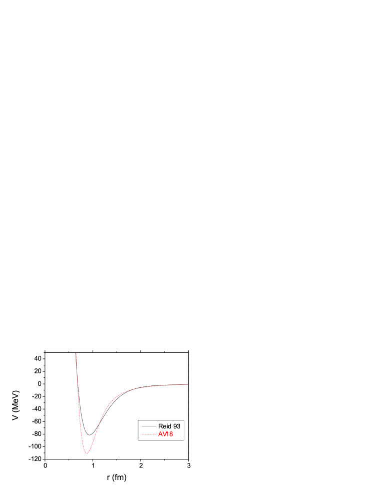
Figure 1: Reid 93 and AV18 ${}^{1}\emph{S}_{0}$ nn potentials.

A much more serious problem arises due to the hard-core short range part of the nuclear potentials (see Figs. 1). Notably, the presence of the $e^{{-cr^{2}}}$ terms in AV18 AV18 and AV14 AV14 models settles that for CS with $\theta>45^{\circ}$ these potentials become divergent. Furthermore even for smaller $\theta$ these two models have a strong oscillatory behavior which makes numerics unstable. This can be seen in Fig. 2 where the transformed NN potentials for two different angles are plotted. Note that the number of oscillations as well as their amplitudes increase dramatically with the rotation angle. In this sense Reid 93 model Reid has the best analytical properties with respect to CS, though it provides stable results only for the $\theta\lesssim 35^{\circ}$.

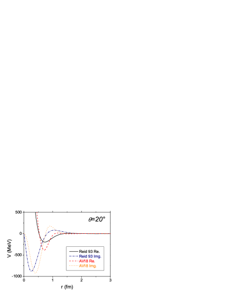
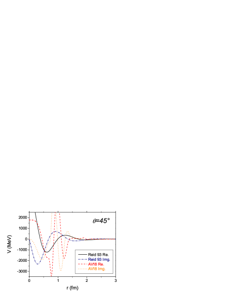
Figure 2: Analytical continuation of the ${}^{1}\emph{S}_{0}$ Reid 93 and AV18 nn potential under the complex scaling transformation eq. (4) with $\theta=20^{\circ}$ and $\theta=45^{\circ}$. One can notice that AV18 potential results into much more oscillating structure than Reid 93.

When treating two-body systems, the numerical complications described above can be avoided by using the so-called ‘smooth-exterior’ complex scaling (SECS) Moiseyev . The problem due to the hard core of the nuclear potentials is overcome by performing scaling operation only in the outside region of the interaction. This method can be implemented by using the following transformation 3n_res_gloe ; Moiseyev :

$$r\rightarrow F(r)$$

with

$$F(r)=r+\left[e^{i\theta}-1\right]\left\{r+\frac{1}{4\eta}\ln\frac{\left[1+e^{2\eta(r-R)}\right]\left[1+e^{-2\eta(r-R)}\right]}{\left[1+e^{2\eta(r+R)}\right]\left[1+e^{-2\eta(r+R)}\right]}\right\}.$$ (12)

where $\eta$ and $R$ are smoothing parameters. However, despite the efficiency of this method when dealing with n=2 problem, it is not easy to implement it in the n=3 Faddeev equations 3n_res_gloe . The problems turned out to be crucial when calculating deeply lying resonances and we were limited to those with $E_{re}/E_{img}\succsim 0.5$.

All the difficulties discussed above are not encountered in the ACCC method, which can be used in principle even to determine subthreshold ($\varepsilon_{res}<0$) resonances. In calculating the input binding energies for determining the Padé approximant (11), one can also scale the total nn potential with a scaling factor $\gamma$ – not necessarily only its attractive part – and consider $\gamma$ as the extrapolation parameter $\gamma\equiv\lambda$.

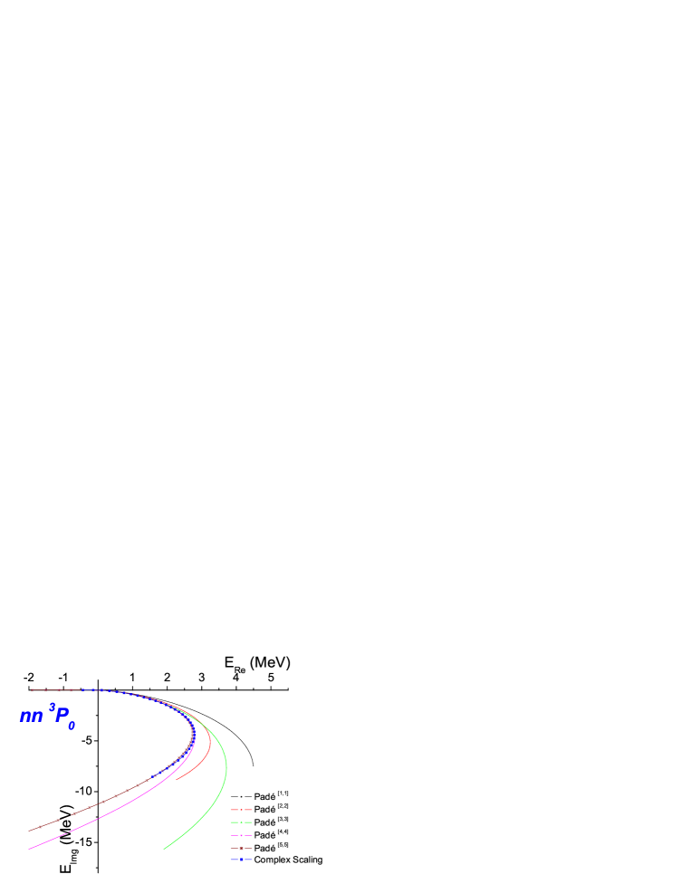
Figure 3: Comparison between ACCC and CS methods for ${}^{3}\emph{P}_{0}$ nn resonance trajectories with Reid93 potential. ACCC results with several Padé orders [N,M] and $\gamma$=6.1 to 1.0 are represented by solid lines. CS results are denoted by squares and correspond to $\gamma$ from 6.1 to 2.7 by steps of 0.1. Star points correspond to [5,5] Padé approximant used in ACCC. They are already very close to CS results: by adding a few terms in the approximant a perfect agreement is reached.

In Figure 3 we compare the results of various order Padé approximant used in (11) with the ones obtained using CS method: dineutron resonance trajectory is depicted for Reid 93 ${}^{3}\emph{P}_{0}$ nn-waves. One can see that a nice agreement is reached between both techniques even when calculating broad resonances, near and beyond the saturation point (where real energy part starts decreasing), provided high order Padé approximant are used. This requirement can not always be met in numerical calculations with realistic interactions, since it implies a very accurate binding energy input. Another critical point of ACCC method, as discussed in Kukulin_book , is that its efficiency highly depends on the accuracy of $\lambda_{0}$ value. The determination of $\lambda_{0}$ is often difficult, since one has to deal with critically bound systems having very extended wave functions. Therefore one has to be rather prudent when applying this method and always check if Padé extrapolation converges.

Table 1: Critical enhancement factors $\gamma_{c}$ required to bind dineutron in various states and for different NN realistic interaction models in use.

	Nijm II	Reid 93	AV14	AV18
${}^{2}n(^{1}S_{0})$	1.088	1.087	1.063	1.080
${}^{2}n(^{3}P_{0})$	5.95	5.95	5.46	6.10
${}^{2}n(^{3}PF_{2})$	3.89	4.00	4.30	4.39
${}^{2}n(^{1}D_{2})$	9.28	9.22	9.54	10.20

Before starting to analyze three-neutron system it could be useful to discuss the basic properties of dineutron and nn interaction in general. As mentioned above, dineutron is almost bound in the ${}^{1}\emph{S}_{0}$ state: one should enhance the nuclear potential only by a factor $\gamma_{c}\approx 1.08$ to make it bound (see Table 1). Notice the very good agreement for the critical enhancement factors $\gamma_{c}$ obtained by different local NN-interaction models. Only AV14 slightly deviates from the other models, due to its charge invariance assumption: the potential being adjusted to reproduce neutron-proton (np) scattering data, ignores the fact that experimental ${}^{1}\emph{S}_{0}$ nn scattering length is smaller in magnitude than np one nn_scl4 . The spherical symmetry of this state makes that when $\gamma\to 1$, i.e. for the physical value of the potential, the bound state pole moves staying on the imaginary $k$-axis and becomes a virtual state, not a resonance. The approximate position of this state can be evaluated from the nn scattering length by means of the relation $E_{virt}\approx\frac{\hbar^{2}}{ma_{nn}^{2}}$. The results thus obtained together with the exactly calculated virtual state energies are given in Table 2.

Table 2: Nuclear model predictions for nn scattering length (in fm) as well as corresponding virtual state (in MeV), evaluated from scattering length and calculated exactly.

	Nijm II	Reid 93	AV14	AV18
$a_{nn}(^{1}S_{0})$	-17.57	-17.55	-24.02	-18.50
${\hbar^{2}}/(ma^{2}_{nn})$	0.134	0.135	0.072	0.121
$E_{virt}(^{1}S_{0})$	0.1162	0.1165	0.0647	0.1055

In fact, multineutron physics being in low energy regime, is dominated by the large nn scattering length value ($a_{nn}$). The wave function has only a small part in the interaction region (effective range $r_{0}<<a_{nn}$) and therefore marginally depends on the particular form that the nn ${}^{1}\emph{S}_{0}$-potential can take, once $r_{0}$ and $a_{nn}$ are fixed Thesis . On the other hand $r_{0}$ is controlled by the theory – the pion Compton-wavelength – and $a_{nn}$ is constrained by the experiment. These effective range theory arguments Platter show that one should not rely on the modifications of ${}^{1}\emph{S}_{0}$ waves to favor the possible existence of bound or resonant multineutron states.

P-waves of nn interaction are extremely weak and this turns to be a major reason why multineutrons are not bound Thesis . Neutron-neutron interaction in ${}^{3}\emph{P}_{1}$ channel is even repulsive, whereas potentials in ${}^{3}\emph{PF}_{2}$ and ${}^{3}\emph{P}_{0}$ channels should be multiplied by considerably large factors – $\gamma=[3.9-4.4]$ and $[5.5-6.1]$ respectively (see Table 1) – to force dineutron’s binding. The centrifugal barrier moves these artificially bound states into resonances when $\gamma$ is slightly reduced from its critical value.

Dineutron resonance trajectories for ${}^{3}P_{0}$ and ${}^{3}PF_{2}$ states are displayed respectively in Figures 4 and 5. They have been obtained with CS and ACCC methods and different NN interaction models. By using a high order Padé approximant and accurate ${{}^{2}n}$ binding energies input in the ACCC method, we observe a perfect agreement between these two techniques. Due to the limitations in the rotation angle $\theta$, CS method was applied only up to $\gamma=2.7$. The corresponding resonance positions obtained with different NN models are explicitly indicated in the figures. One should note that the resonance trajectories in both states have similar shapes. When decreasing $\gamma$ from its critical value $\gamma_{c}$, the resonance width starts departing slowly from zero and then increases linearly. On the other hand, the real part of the resonance energy – $\varepsilon_{res}$ – first grows linearly with $\gamma_{c}-\gamma$. Afterwards, this growing saturates and reach a maximum value from where it quickly decreases, vanishes and becomes negative. ACCC method allows to follow the resonance trajectories up to the physical value $\gamma=1$ at which the dineutron states are deeply subthreshold. However, the transition to the third energy quadrant happens at a value $\gamma^{\prime}_{c}$ well above. Some resonance trajectory properties obtained using ACCC method are summarized in Table 3. Note that in none of Figures 4 and 5 the resonance trajectories are plotted until the physical value $\gamma=1$.

It is clear from results given in Table 3 that the existence of any observable P-wave dineutron resonance is excluded: only subthreshold poles with large widths persist, making such structures physically meaningless. It is worth noticing recent few-nucleon scattering calculations indicating that a good description of $3N$ and $4N$ scattering observables, would require stronger NN P-wavesP_waves_Gloe ; P_waves_Pisa ; Thesis . However the modifications involved – less than 20% – let the dineutron resonances still subthreshold

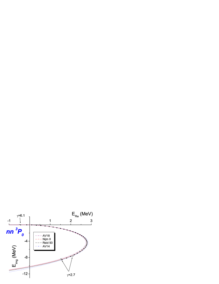
Figure 4: Dineutron ${}^{3}\emph{P}_{0}$ resonant trajectories in complex energy plane for AV14, NijmII, Reid 93 and AV18 nn interactions. Solid dot symbols correspond to $\gamma$ values from 6.1 to 2.7 by steps of 0.1 obtained with CS method and Reid 93. Continuous lines represent ACCC results. ACCC and CS results superimpose up to $\gamma$=2.7 point, the limit of CS applicability.

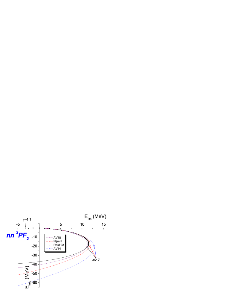
Figure 5: Dineutron ${}^{3}\emph{PF}_{2}$ resonant trajectories in complex energy plane, displayed using the same conventions as in figure 4.

Table 3: Enhancement factor values ($\gamma^{\prime}_{c}$) at which dineutron resonances become subthreshold ($\varepsilon_{res}=0$), and imaginary energy values E${}_{img}(\gamma^{\prime}_{c})$ at this point (MeV). Resonance energy E_res for physical nn interaction (i.e. at $\gamma=1$) obtained using ACCC method.

	${}^{3}P_{0}$				${}^{3}PF_{2}$
	Nijm II	Reid 93	AV14	AV18	Nijm II	Reid 93	AV14	AV18
$\gamma^{\prime}_{c}$	2.27	2.26	2.08	2.24	1.64	1.71	1.46	1.73
E${}_{img}(\gamma^{\prime}_{c})$	-10.2	-10.3	-10.6	-10.2	-45.6	-36.9	-56.2	-40.3
E${}_{res}(\gamma=1)$	-14.1-17.2i	-14.2-18.5i	-10.3-18.1i	-12.1-18.0i	-20.5-64.8i	-15.9-39.9i	-17.9-80.1i	-34.1-45.4i

One should remark the astonishing similarity for the P-wave dineutron resonance trajectories obtained with NN potientials having quite a different shapes (see Fig. 1). ${}^{3}\emph{P}_{0}$ curves for the three charge symmetry-breaking models considered superimpose, whereas for ${}^{3}\emph{PF}_{2}$ they separate only when very large resonance energies are reached. Enhancement factors employed in tracing these curves are unphysically large and produce very broad resonances: ${}^{3}\emph{P}_{0}$ state moves into third energy quadrant at $E_{img}\sim 10$ MeV, while in ${}^{3}\emph{PF}_{2}$ case this value goes beyond 35 MeV.

Two neutron states with orbital angular momentum $\ell$=2, can be realized only in singlet state (${}^{\emph{1}}$D${}_{\emph{2}}$). This state is dominated by a sizeable centrifugal barrier and the critical enhancement factors to bind dineutron ($\gamma_{c}$) is considerably large (see Table 1). The central effective potentials

$$V_{eff}(r)=V_{nn}(r)+\frac{\hbar^{2}}{m_{n}}\frac{\ell(\ell+1)}{r^{2}}$$

in this and higher angular momentum nn partial waves are smoothly decreasing functions, without any dips, implying without further calculation that dineutron can not have $\ell\geqslant$2 observable resonances in the 4th quadrant.

As mentioned in section II we cannot obtain numerically all the eigenvalue spectra of the 3n problem. Only a few specific eigenvalues of the linear system (9) can be extracted by applying iterative methods. When using the CS method, these techniques do not allow us a-priori to separate eigenvalues related to the resonances from the spurious ones related to the rotated continuum. In order to force the numerical procees to converge towards the resonance position we have to initialize it with a rather accurate guess value. This obliged us to follow the procedure described in 3n_res_gloe : first we bind three neutrons by artificially making nn interaction stronger, and then we gradually remove the additional interaction and follow the trajectory of this state. Note, that in bound state calculations one can use linear algebra methods determining the extreme eigenvalues of the spectra (e.g. Lanczos or Power-method), whereas resonance eigenvalue in the CS matrices is not anymore an extreme one.

By enhancing the ${}^{\emph{1}}\emph{S}_{\emph{0}}$ nn-potential there is no way to bind three neutrons without first binding dineutron. On the other hand, as quoted before, this wave is controlled both by theory and experiment and modifications of its form can not affect multineutron physics. Three-neutron can neither be bound if we keep the ${}^{\emph{1}}$S${}_{\emph{0}}$ interaction unchanged, and multiply all nn P-waves with the same enhancement factor; by doing so, dineutron will be bound in ${}^{3}\emph{PF}_{2}$ channel before three-neutron was. In view of that, we have tried to enhance only one of P interactions, keeping the usual strengths for the other ones. The ${}^{3}\emph{P}_{1}$ potential is purely repulsive and its enhancement can not give any positive effect. The ${}^{3}\emph{P}_{0}$ enhancement gives null result as well: dineutron is always bound before any ${}^{3}n$ states is formed. Only enhancing ${}^{3}\emph{PF}_{2}$ channel we managed to bind trineutron without first binding dineutron and this happens in the $J^{\pi}=\frac{3}{2}^{-}$ ${}^{3}n$ state alone. These properties turned to be general in the four realistic interactions (AV14, Reid 93, Nijm II and AV18) we have investigated.

The critical ${}^{3}\emph{PF}_{2}$ enhancement factors $\gamma_{c}$ required to bind ${{}^{3}n}$ are summarized in Table 4. They are so large that dineutron, although unbound, is already resonant; the corresponding resonance positions are summarized in the bottom line of this Table. One can remark, once again, the rather good agreement between the different model predictions. This fact, as well as the similarity in the dineutron case, predictions suggest that the different realistic local-interaction models would provide a good qualitative agreement in multineutron physics as well. Therefore, in further analysis of three-neutron resonances we will rely on a single interaction model. In this respect, Reid 93 model is the most suited, since it possess the best analytical properties and consequently provides the most stable numerical results for CS method.

Table 4: Critical enhancement factors $\gamma_{c}$ required for ${}^{3}\emph{PF}_{2}$ nn channel to bind $J^{\pi}=\frac{3}{2}^{-}$ three-neutron and corresponding $J^{\pi}=2^{-}$ dineutron resonance positions (MeV).

	Nijm II	Reid 93	AV14	AV18
$\gamma_{c}({{}^{3}n})$	3.61	3.74	3.86	3.98
E(${}^{2}n$) MeV	5.31-2.41$i$	5.41-2.52$i$	5.20-2.49$i$	4.83-2.31$i$

As mentioned, above only a $\frac{3}{2}^{-}$ three-neutron state can be bound by enhancing single NN interaction, without first binding dineutron. In Figure 6 we trace the ${}^{3}n$ resonance trajectory (full circles) for this state when the ${}^{3}\emph{PF}_{2}$ enhancement factor changes from 3.7 to 2.8 with step of 0.05. Result were obtained using CS methods. Extending the calculations to smaller $\gamma$ values generated numerical instabilities, due to the necessity to scale Faddeev equations with ever increasing $\theta$. It can be seen however, that this trajectory bends faster than the analogous one for the dineutron in ${}^{3}\emph{PF}_{2}$ state, therefore indicating that it will finish in the third energy quadrant with Re(E)$<$0.

Three-neutron can also be bound in states $\frac{3}{2}^{+}$ and $\frac{1}{2}^{-}$ states by enhancing combined ${}^{3}\emph{PF}_{2}$ and ${}^{3}\emph{P}_{1}$ waves. However such a binding is a consequence of strongly resonant dineutrons in both mentioned waves. These resonances are very sensible to the small reductions of the enhancement factor and they quickly vanish leaving only the dineutron ones.

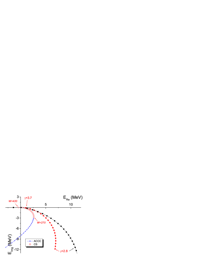
Figure 6: $J^{\pi}=3/2^{-}$ three-neutron state resonance trajectory obtained when reducing the strength $W$ of phenomenological Yukawa-type force (open circles for CS and solid line+star points for ACCC methods). Trajectory depicted by full circles represents one obtained using CS, when reducing enhancement factor $\gamma$ for ${}^{3}\emph{P}_{2}-^{3}\emph{F}_{2}$ nn interaction . Trajectory depicted by full squares is dineutron resonance path in ${}^{3}\emph{P}_{2}-^{3}\emph{F}_{2}$ channel, obtained by enhancing nn-interaction in these waves. Presented results are based on Reid 93 model.

In order to systematically explore the possible existence of resonances in all the three-neutron states, we let unchanged the original NN-interaction and force the binding by means of a phenomenological attractive three-body force. We have assumed the latter to have an hyperradial Yukawa form:

$$V_{3n}=-W\frac{e^{-{\rho\over\rho_{0}}}}{\rho},\text{ with }\rho=\sqrt{x_{ij}^{2}+y_{ij}^{2}}$$ (13)

with $\rho_{0}=2$ fm. In this way, dineutron physics is not affected.

Table 5: Critical strengths $W_{0}$ in MeV$\cdot$fm of the phenomenological Yukawa-type force of eq. (13) required to bind three-neutron in various states. Parameter $\rho_{0}$ of this force was fixed to 2 fm. $W^{\prime}$ are the values at which three-neutron resonances become subthreshold ones, whereas $B_{trit}$ are such 3NF corresponding triton binding energies in MeV.

$J^{\pi}$	$\frac{1}{2}^{+}$	$\frac{3}{2}^{+}$	$\frac{5}{2}^{+}$	$\frac{1}{2}^{-}$	$\frac{3}{2}^{-}$	$\frac{5}{2}^{-}$
$W_{0}$	307	1062	809	515	413	629
$W^{\prime}$	152	-	329	118	146	277
$B_{trit}$	21.35	-	44.55	17.72	20.69	37.05

In table 5 we summarize the critical values $W_{0}$ of the strength parameter $W$ for which the three-neutron system is bound in different states. Corresponding resonance trajectories obtained by gradually reducing parameter $W$ are traced in Fig. 7. As in previous plots, CS results are presented by separate solid points, whereas ACCC ones are using continuous line and star points. One can see a very nice agreement between the two methods except for the $J^{\pi}=\frac{5}{2}^{+}$ state, where a discrepancy between two methods manifests at large energy. This is probably an artifact of the very strong 3NF used. Such a force confines the three-neutron system inside a $\approx$1.4 fm box, a distance smaller than the 3NF range itself, and starts to compete with the hard-core repulsive part of the nn interaction, making the ACCC method badly convergent for broad resonances. For the $J^{\pi}=\frac{3}{2}^{+}$ state, due to the even larger $W$ values, ACCC method has not been used.

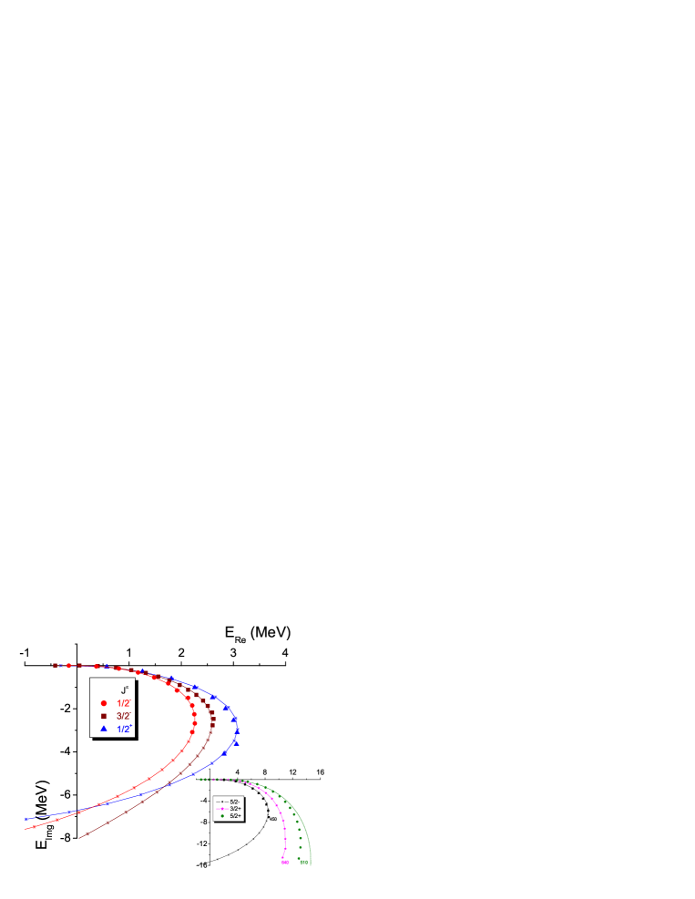
Figure 7: Three-neutron resonance trajectories obtained when varying the strength $W$ of Yukawa-type 3NF. Results obtained using CS method are plotted with solid points. For the $J^{\pi}=1/2^{-}$ state, $W$ varies from 520 to 300 MeV$\cdot$fm by steps of 20 MeV$\cdot$fm, denoted for shortness [520,300,20]. For $J^{\pi}=3/2^{-}$, W is in the range $[420,270,10]$ and for $J^{\pi}=1/2^{+}$ in [310,210,10]. Other 3n states – depicted in the smaller figure – require considerably stronger 3NF to be bound and result in large resonance energies values. For $J^{\pi}=5/2^{-}$ $W$ changed in [610,450,10], for $J^{\pi}=5/2^{+}$ $W$ in [810,750,10] and then in [750,510,20], and for $J^{\pi}=3/2^{+}$ in [1060,800,20] and [800,640,40]. ACCC method results are presented by solid lines, supported by star points.

One can remark that resonance trajectories have similar shapes for all the three-neutron states, with the resonance poles tending to slip into the third quadrant ($\varepsilon_{res}<0$) well before $W$ equals 0, i.e. when the additional 3NF are fully removed and only NN-interaction remains. In Table 5 are also given the values $W^{\prime}$, obtained using ACCC method, at which ${{}^{3}n}$ resonances become subthreshold ($\varepsilon_{res}=0$). These values are still rather large, strongly exceeding what could be expected for realistic 3NF. To illustrate how strongly such 3NF violate the nuclear properties, we give in the last row of the Table, the triton binding energies, obtained supposing that the same 3NF with strength $W^{\prime}$ acts on it. These energies would be even larger if the range parameter $\rho_{0}$ taken in our 3NF model had had smaller and more realistic values.

The preceding results demonstrate that realistic NN-interaction models exclude the existence of observable three-neutron resonances. In Csoto ${{}^{3}n}$, resonance in $\frac{3}{2}^{+}$ state was claimed at $E=14-13i$ MeV for the non-realistic Minnesota potential. Our results using realistic nn interaction contradict however the existence of such a resonance. A very strong additional interaction is required to bind three-neutron in $J^{\pi}=\frac{3}{2}^{+}$ state. Removing this interaction, the imaginary part of the resonance grows very rapidly while its real part saturates rather early (starting with $\approx$1060 MeV$\cdot$fm, it reaches its maximal value at $W\approx$720 MeV$\cdot$fm). Once this saturation point is reached, the resonance trajectory moves rapidly into the third quadrant.

The results shown in Figure 7 represent the ${}^{3}n$ resonance trajectories only partially, without following them to their final positions $W=0$, i.e. when the additional interaction is completely removed. The reason is that these positions are very far from the bound state region, thus requiring many terms in Padé expansion to ensure an accurate ACCC result. In principle, one could always imagine that these trajectories turn around and return to the fourth quadrant with positive real parts. Although we have never encountered such a scenario in practical calculations, we are not aware of any rigorous mathematical proof forbiding it and it cannot consequently be excluded.

Such a kind of evolution seems however very unlikely in a physical case of interest. The resonance trajectories should indeed exhibit a very sharp behavior once entered in the third quadrant whereas all our results indicate always a rather smooth variation.

In this study we have deliberately omitted the use of realistic 3NF models. The reason is that such forces are not completely settled yet, specially for pure neutron matter. In addition, we should remark that the UIX UIX 3NF acts repulsively for multineutron systems Thesis . The more recent Illinois 3NF contains charge symmetry breaking (CSB) and considerably improves the underbinding problem of neutron rich nuclei present for AV18+UIX PPWC_PRC64 . However, even strongly CSB realistic 3NF would be by order too weak to make three-neutron system resonant. The reason of weak 3NF efficiency in multineutron physics is that such force requires configurations when all three neutrons are close to each other, whereas such structures are strongly suppressed by Pauli principle.

Finally, one can expect that the different ways used to artificially generate bound states could give rise to different resonance trajectories. Some resonance could thus have existed which are missed in our approach. To investigate such a possibility we have chosen a $J^{\pi}=\frac{3}{2}^{-}$ resonance, obtained by means of the phenomenological 3NF force (13) with $W=360$ MeV$\cdot$fm. Then we gradually reduce $W$ to zero, increasing at the same time the enhancement factor for the ${}^{3}\emph{PF}_{2}$ potential from $\gamma=1$ to $\gamma=3.7$. The resonance trajectory obtained this way is plotted (cross circles) in Figure 8 together with the resonance curves obtained by additional 3NF only (open circles) and by enhancing only ${}^{3}\emph{PF}_{2}$ nn potential (full circles). Once 3NF was completely removed, the resonance pole joined the curve obtained with enhanced ${}^{3}\emph{PF}_{2}$ channel. Note that the structure of bound state obtained with 3N force and by enhancing P-waves are quite different. 3NF requires very dense and spherical symmetric neutron wave functions. This is the reason why the $\frac{1}{2}^{+}$ state is more favorable than $\frac{3}{2}^{-}$ (see Table 5) to bind three-neutron when using such an additional force.

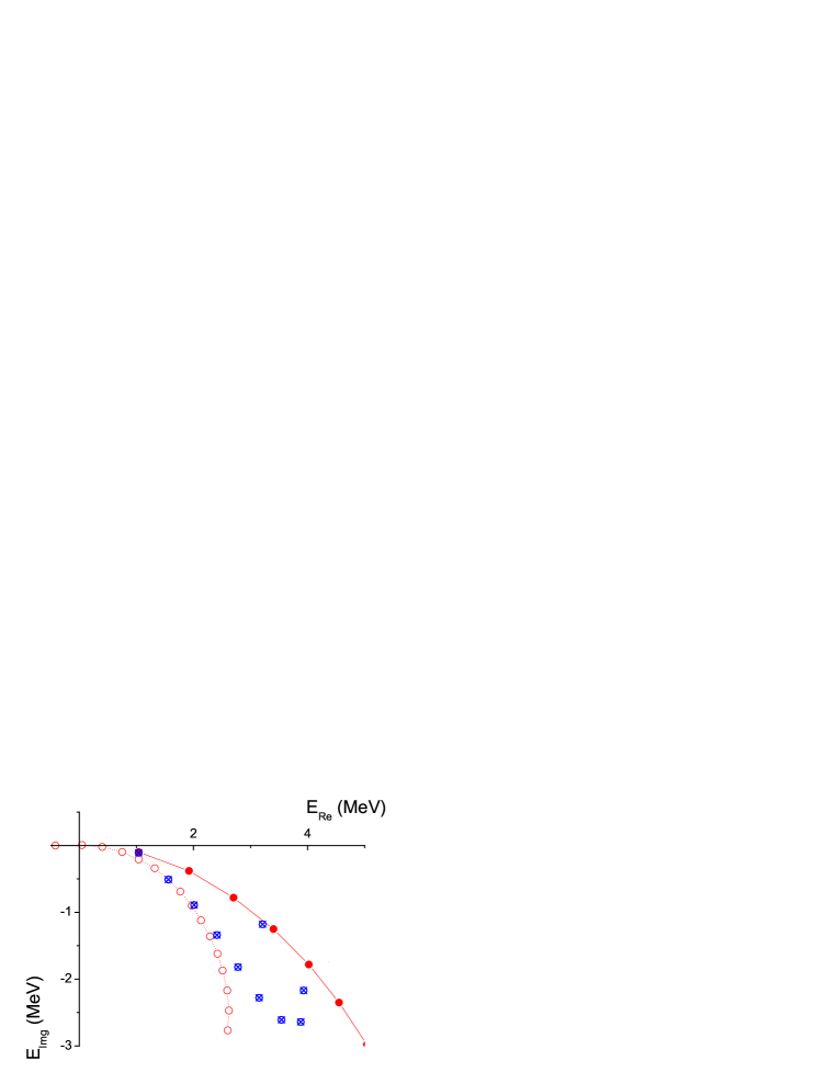
Figure 8: $J^{\pi}=3/2^{-}$ 3n resonance trajectories obtained when reducing the strength $W$ in the Yukawa-type 3NF (open circles) and enhancing ${}^{3}\emph{PF}_{2}$ nn interaction (full circles). Crossed circles indicate the resonance path obtained when starting from $(W=360\mbox{ MeV$\cdot$fm},\gamma=1)$ and going gradually to $(W=0,\gamma=3.7)$.

IV Conclusion

A systematic study of three-neutron resonances using realistic NN-interaction models was presented. The search of resonance positions was carried out by artificially enhancing the interaction between the neutrons in such a way that the three-neutron system becomes bound. Then, by gradually removing the additional interaction we followed the path of the resonance energy located in the third and fourth quadrants of the second Riemann sheet.

Two different methods were successfully applied to trace resonance trajectories, namely the Complex Scaling (CS) and the Analytical Continuation in the Coupling Constant (ACCC). They provided results in very good agreement. Two alternative ways were also explored to enhance the interaction between neutrons: in one of them, the three-neutron system was bound by adding a phenomenological three-nucleon force (3NF) and in the other one the binding was obtained by enhancing the interaction in some NN partial waves.

All ${{}^{3}n}$ resonance trajectories, for states up to $J=5/2$, were shown to move into the third energy quadrant (Re(E)$<0$) becoming subthreshold resonances, well before the additional interaction is fully removed. Our results clearly demonstrate that the current realistic interactions exclude the possible existence of bound as well as resonant three-neutron states. To push the three-neutron resonance out of the subthreshold region, such models should already be strongly violated. These findings support the results of Ref Glockle_Hem for simplified NN-interaction model.

The possible existence of observable four-neutron (tetraneutron) resonance seems rather doubtful as well, since for such a system to be artificially bound one requires almost as large enhancement factors as in the three-neutron case Thesis . Still, such a possibility can not be completely excluded, since the tetraneutron is favored due to presence of two almost bound dineutron pairs. Moreover, recent experiment on ${}^{8}He(d,{{}^{6}Li})4n$ reaction shows an excess of low energy ⁶Li nuclei with respect to what one could expect from a phase space analysis Exxon . The presence of events associated with a resonant tetraneutron state was suggested. The possible existence of such structures will be explored in a forthcoming work.

Acknowledgements: Numerical calculations were performed at Institut du Développement et des Ressources en Informatique Scientifique (IDRIS) from CNRS and at Centre de Calcul Recherche et Technologie (CCRT) from CEA Bruyères le Châtel. We are grateful to the staff members of these two organizations for their kind hospitality and useful advices.

References

- (1) C. R. Howell et. al.: Phys. Lett. B 444 (1998) 252.
- (2) R. Guardiola and J. Navarro: Phys. Rev. Lett. 84 (2001) 1144.
- (3) A.A. Oglobin, Y.E. Penionzhkevich: Treatise on Heavy-Ion Science (vol. 8): Nuclei Far From Stability, Ed. D. A. Bromley (Plenum Press, New York, 1989) 261.
- (4) F. M. Marqués et. al: Phys. Rev.C 65 (2002) 044006
- (5) R. Lazauskas: PhD Thesis, Université Joseph Fourier, Grenoble (2003); http://tel.ccsd.cnrs.fr/documents/archives0/00/00/41/78/.
- (6) S.C. Pieper: Phys. Rev. Lett.90 (2003) 252501.
- (7) C.A. Bertulani, V. Zelevinsky: J.Phys. G29 (2003) 2431.
- (8) N. K. Timofeyuk: J. Phys. G 29 (2003) L9.
- (9) D. R. Tilley, H.R. Weller and H.H. Hasan: Nucl. Phys. A 474 (1987) 1.
- (10) M.Yuly et. al: Phys. Rev. C 55 (1997) 1848.
- (11) J. Sperinde, D. Frederickson, R. Hinkis, V. Perez-Mendez and B. Smith: Phys. Lett. 32 B (1970) 185.
- (12) A. Stetz et al.: Nucl. Phys. A 457 (1986) 669.
- (13) E. Rich et al.: Procedings to Exxon Conference (4-12 July 2004).
- (14) A. Csótó, H. Oberhummer and R.Pichler: Phys. Rev. C 53 (1996) 1589.
- (15) S.A. Sofianos, S.A. Rakityansky and G.P. Vermaak: J. Phys. G. Nucl. Part. Phys. 23 (1997) 1619.
- (16) H. Witała, W. Glöckle: Phys. Rev. C 60 (1999) 024002.
- (17) A. Hemmdan, W. Glöckle and H. Kamada: Phys. Rev. C 66 (2002) 054001.
- (18) D. Gogny, R.Pires and R. de Tourreil: Phys. Lett. 32 B (1970) 591.
- (19) N. Moiseyev: Phys. Rep. 302 (1998) 211.
- (20) Y. K. Ho: Phys. Rep. 99 (1983) 1.
- (21) L.D. Faddeev: Zh. Eksp. Teor. Fiz. 39, (1960) 1459 [Sov. Phys. JETP 12, (1961) 1014.
- (22) H.P. Noyes: in Three-Body problems in Nuclear and particle physics, edited by J.S.C. McKee and P.M. Rolph (North-Holland, Amsterdam, 1970) p.2.
- (23) F. Ciesielski, J. Carbonell: Phys. Rev. C 58 (1998) 58.
- (24) C. de Boor: A Practical Guide to Splines (Springer-Verlag, Berlin 1978).
- (25) V.I. Kukulin, V.M. Krasnopolsky: J. Phys. A 10 (1977) L33
- (26) V.I. Kukulin, V.M. Krasnopolsky and M. Miselkhi: Sov. J. Nucl. Phys. 29 (1979) 421
- (27) V.M. Krasnopolsky and V.I. Kukulin: Phys. Lett. 69A (1978) 251.
- (28) V.I. Kukulin, V.M. Krasnopolsky and M. Miselkhi: Sov. J. Nucl. Phys. 30 (1979) 740
- (29) V.I. Kukulin, V.M. Krasnopolsky and J. Horáček: Theory of Resonances, principles and applications (Kluwer 1989)
- (30) G.A. Baker: Advances in theor. phys. (Academic, New York, London, 1965) Vol 1, p.1.
- (31) L. Platter, H.W. Hammer and Ulf-G. Meißner: Phys. Rev. A 70 (2004) 052101
- (32) H. Witała, W. Glöckle: Nucl. Phys. A 528 (1991) 48.
- (33) W. Tornow, H. Witała and A. Kievsky: Phys. Rev. C 57 (1998) 555.
- (34) R.B. Wiringa, R.A. Smith and T.L. Ainsworth: Phys. Rev. C 29 (1984) 1207.
- (35) R.B. Wiringa, V.G.J. Stoks, and R. Schiavilla: Phys. Rev. C 51 (1995) 38.
- (36) V.G.J. Stoks, R.A.M. Klomp, M.C.M. Rentmeester and J.J. de Swart: Phys. Rev. C 48 (1993) 792.
- (37) B.S. Pudliner, V.R. Pandharipande, J. Carlson and R.B. Wiringa: Phys. Rev. Lett. 74 (1995) 4396.
- (38) S.C. Pieper, V.R. Pandharipande, R.B. Wiringa, J. Carlson, Phys. Rev. C 64 (2001) 014001-1