Three-body resonant radiative capture reactions in astrophysics

Abstract

We develop the formalism based on the S-matrix for $3\rightarrow 3$ scattering to derive the direct three-body resonant radiative capture reaction rate. Within this formalism the states, which decay only/predominantly directly into three-body continuum, should also be included in the capture rate calculations. Basing on the derivation, as well as on the modern experimental data and theoretical calculations concerning ¹⁷Ne nucleus, we significantly update the reaction rate for ¹⁵O($2p$,$\gamma$)¹⁷Ne process in explosive environment. We also discuss possible implementations for the ¹⁸Ne($2p$,$\gamma$)²⁰Mg, ³⁸Ca($2p$,$\gamma$)⁴⁰Ti, and ⁴He($n\alpha$,$\gamma$)⁹Be reactions.

I Introduction

The reactions of the three-body radiative capture may play a considerable role in the rapid nuclear processes which take place in stellar media under the conditions of high temperature and density. The possibility to bridge the waiting points of the $rp$-process in the explosive hydrogen burning by the $2p$ radiative capture reactions was discussed in Ref. gor95 . The reactions ¹⁵O($2p$,$\gamma$)¹⁷Ne, ¹⁸Ne($2p$,$\gamma$)²⁰Mg, and ³⁸Ca($2p$,$\gamma$)⁴⁰Ti could be a more efficient way to “utilize” ¹⁵O, ¹⁸Ne, and ³⁸Ca, than to wait for their $\beta^{+}$ decay (corresponding lifetimes are 122, 1.67, and 0.44 seconds). The ⁴He($n\alpha$,$\gamma$)⁹Be reaction has been found to be important for building heavy elements in the explosions of supernovae woo94 ; tak94 . This reaction has been several times theoretically considered in the recent years fow75 ; gor95a ; cau88 ; efr98 ; ang99 ; buc01 .

The three-body radiative capture is a very improbable process. It can only be important if the sequence of the two-body radiative captures to the bound states is not possible. This happens if the bound intermediate system does not exist (along the driplines the continuum ground states are not uncommon). The three-body radiative capture can proceed sequentially via the intermediate resonances or directly from the three-body continuum. The later is the inverse process to the “true” two-proton radioactivity gol60 , which studies are active now gri00 ; gri01 ; gri02 ; pfu02 ; gio02 ; chr02 ; gri03 ; gri03a ; bro03 ; gri03b . The relations between sequential and direct mechanisms of two-proton decay are discussed in details in Refs. gri01 ; gri03a .

In the modern literature exists some misunderstanding about the role of the direct three-body capture in the theoretical calculations of the three-body radiative capture rates. In the most cases this misunderstanding does not lead to any significant problems. However, in some situations the difference is sufficiently large. In our opinion the origin of the misunderstanding is the following. The accurate formulae for the resonant three-body capture are known for a long time (see e.g. Ref. fow67 ). But nowadays they does not seem to be always interpreted completely correctly. The possible reason is that for nonresonant capture calculations the sequential capture formalism is used nom85 ; gor95 ; gor95a ; ang99 ; buc01 . At some stage it has become considered as obtained in more general assumptions (see e.g. Ref. nom85 ) than the derivation of Ref. fow67 , based on complete thermal equilibrium and detailed balance.

In this paper we use formalism based on the S-matrix for $3\rightarrow 3$ scattering to derive the reaction rates for the three-body resonant radiative capture. In this approach the right way of using these formulae becomes evident. We find that the direct and sequential capture mechanisms are complementing each other. In the cases when the sequential process is prohibited energetically or suppressed dynamically the sequential formalism should underestimate the rate. Among the processes, where significant differences with previous calculations can be found are reactions leading to ¹⁷Ne and ⁴⁰Ti.

The unit system $\hbar=c=1$ is used in the article.

II Three-body radiative capture

The derivations provided below are relatively trivial. Those of Section II.1 can be found e.g. in Refs. nom85 ; gor95 . They are presented, however, in much details to provide unified notations, simplify the reading of the paper and to avoid any possible misinterpretation.

II.1 Sequential capture

The abundance $Y_{A+2}$ for the nucleus with mass number $A+2$ due to the sequential two-proton capture reaction on the nucleus with mass number $A$ is defined via three-body reaction rate $\left\langle\sigma_{pp,\gamma}v\right\rangle$ as (see e.g. Ref. fow67 ):

$$\dot{Y}_{A+2}=(1/2)\;N_{A}^{2}\,\rho^{2}\;\left\langle\sigma_{pp,\gamma}v\right\rangle\;Y_{p}^{2}Y_{A},$$ (1)

where $\rho$ is density and $N_{A}$ is Avogadro number. The two-proton reaction rate is defined for sequential capture of protons (for example in gor95 ) by

$$\left\langle\sigma_{pp,\gamma}v\right\rangle=2\sum_{i}\frac{\left\langle\sigma_{p,p}v\right\rangle_{i}}{\Gamma_{p,i}}\left\langle\sigma_{p,\gamma}v\right\rangle_{i}\;.$$

This expression is a consequence of the rate equations for the resonance number $i$:

$$\dot{Y}_{A+1}^{(i)} = N_{A}\,\rho\;\left\langle\sigma_{p,p}v\right\rangle_{i}\;Y_{p}Y_{A}-\Gamma_{p,i}Y_{A+1}^{(i)}$$

$$\dot{Y}_{A+2} = \sum_{i}N_{A}\,\rho\;\left\langle\sigma_{p,\gamma}v\right\rangle_{i}\;Y_{p}Y_{A+1}^{(i)}$$ (2)

and the assumption about thermodynamic equilibrium for the intermediate resonant states $\dot{Y}_{A+1}^{(i)}=0$.

The standard expression for cross section of the resonance reaction with entrance channel $\alpha$ and exit channel $\beta$ is

$$\sigma(E)=\frac{\pi}{k_{12}^{2}}\,\frac{\Gamma_{\alpha}\Gamma_{\beta}}{(E-E_{R})^{2}+\Gamma^{2}/4}\,\frac{2J_{2R}+1}{(2J_{1}+1)(2J_{2}+1)}\,,$$ (3)

where $J_{1}$ and $J_{2}$ are the total spins of incoming particles and $J_{2R}$ is the total spin of the resonance.

In the case of intermediate capture into the narrow proton resonance number $i$ (which also decays practically only via proton emission) $\Gamma_{\alpha}=\Gamma_{\beta}=\Gamma_{p,i}\,$, and

$$\left\langle\sigma_{p,p}v\right\rangle_{i}=\int v\,\sigma_{i}(E_{12})\,w(k_{12})\,d^{3}k_{12}=\left(\frac{A_{1}+A_{2}}{A_{1}A_{2}}\right)^{3/2}$$

$$\times\;\frac{2J_{2R,i}+1}{2(2J_{I}+1)}\left(\frac{2\pi}{mkT}\right)^{3/2}\!\exp\left[-\frac{E_{2R,i}}{kT}\right]\Gamma_{p,i}\,,\quad$$ (4)

where $J_{I}$ is the total spin of the initial (core) nucleus and $J_{2R,i}$ is the total spin of the resonance number $i$ in the core+$p$ system. The Boltzmann distribution over the relative motion momentum $k_{12}=\sqrt{2m_{12}E_{12}}$ is

$$w(k_{12})={(2\pi m_{12}kT)^{-3/2}\exp[-E_{12}/kT]}\,,$$

and we approximate the integral over the resonance profile as

$$\int_{-\infty}^{\infty}\frac{dE}{(E-E_{R})^{2}+\Gamma^{2}/4}=\frac{2\pi}{\Gamma}\,.$$

The reaction rate for the subsequent capture of the second proton on the system core+$p$ in the resonant state number $i$ and the following gamma emission is:

$$\left\langle\sigma_{p,\gamma}v\right\rangle_{i} = \left(\frac{A_{1}+A_{2}+A_{3}}{(A_{1}+A_{2})A_{3}}\right)^{3/2}\!\!\!\!\frac{2J_{F}+1}{2(2J_{2R,i}+1)}\left(\frac{2\pi}{mkT}\right)^{3/2}$$ (5)

$$\times \,\exp\left[-(E_{3R}-E_{2R,i})/kT\right]\;\Gamma_{\gamma}\Gamma_{p,i}^{\prime}/\Gamma_{3R}\,,$$

where $J_{F}$ is the total spin of the resonance $E_{3R}$ in the core+$2p$ system. $\Gamma_{p,i}^{\prime}$ is the partial width for decay of this state into the binary channel (core+$p$)+$p$, where the core+$p$ system is in the resonant state number $i$. It is easy to find out that the two-proton reaction rate for sequential proton capture (through narrow intermediate resonances) is

$$\left\langle\sigma_{pp,\gamma}v\right\rangle = \left(\frac{A_{1}+A_{2}+A_{3}}{A_{1}A_{2}A_{3}}\right)^{3/2}\!\!\frac{2J_{F}+1}{2(2J_{I}+1)}\left(\frac{2\pi}{mkT}\right)^{3}$$ (6)

$$\times \,\exp\left[-E_{3R}/kT\right]\;\textstyle\left(\Gamma_{\gamma}\sum_{i}\Gamma_{p,i}^{\prime}\right)/\Gamma_{3R}\,.$$

The following features of the rate Eq. (6) should be noted:

(i) The reaction rate does not depend on the number and properties of the intermediate states, but only on the sum of the proton widths for population of these states.

(ii) In the most expected case of the sequential decay mode dominance for the three-body resonance $E_{3R}$ we have $\Gamma_{\gamma}\ll\Gamma_{3R}$, $\Gamma_{2p}\ll\Gamma_{3R}$ ($\Gamma_{2p}$ is the width for the direct decay into $2p$ continuum, the process not proceeding via intermediate core+$p$ resonances) and $\Gamma_{3R}=\sum_{i}\Gamma_{p,i}^{\prime}\,$. So, the reaction rate depends only on gamma width of the three-body resonance.

(iii) Eq. (6) shows that if there exist other significant decay channels for three-body resonance $E_{3R}$, then $\Gamma_{3R}>\sum_{i}\Gamma_{p,i}^{\prime}$ and the production rate decreases. Such possible decay channel is, already mentioned, direct (not via resonances) decay of the three-body resonance $E_{3R}$ into two-proton continuum. Typically this process is suppressed, but there are cases where this process is not suppressed. It can be dominating, or even it can be the only possible decay channel (no intermediate resonances). Such an opportunity is considered in the next Section.

II.2 Direct capture

The abundance $Y_{A+2}$ due to the direct two-proton capture reaction is defined via three-body reaction rate as

$$\dot{Y}_{A+2}=(1/2)\;N_{A}^{2}\,\rho^{2}\;\left\langle\sigma_{2p,\gamma}v\right\rangle\;Y_{p}^{2}Y_{A}.$$ (7)

To derive the cross section of the direct capture from the three-body continuum we use the S-matrix formalism for $3\rightarrow 3$ reaction. The plane wave for three particles can be decomposed over hyperspherical harmonics $\mathcal{I}_{K\gamma}^{LM_{L}}$:

$$\Psi_{3}^{pw}=\exp[\,i\mathbf{k}_{1}\mathbf{r}_{1}+i\mathbf{k}_{2}\mathbf{r}_{2}+i\mathbf{k}_{3}\mathbf{r}_{3}]\,\chi_{S_{1}M_{1}}\chi_{S_{2}M_{2}}\chi_{S_{3}M_{3}}$$

$$=\exp[\,i\mathbf{k}_{cm}\mathbf{R}_{cm}+i\mathbf{k}_{y}\mathbf{Y}+i\mathbf{k}_{x}\mathbf{X}]\,\chi_{S_{1}M_{1}}\chi_{S_{2}M_{2}}\chi_{S_{3}M_{3}}$$

$$=\;\exp[\,i\mathbf{k}_{cm}\mathbf{R}_{cm}]\;\frac{\left(2\pi\right)^{3}}{\left(\varkappa\rho\right)^{2}}\sum_{JM}\,\sum_{KLl_{x}l_{y}SS_{x}}i^{K}J_{K+2}(\varkappa\rho)$$

$$\times\;\mathcal{J}_{KLl_{x}l_{y}SS_{x}}^{JM}(\Omega_{\rho})\,\sum_{M_{L}}\mathcal{I}_{Kl_{x}l_{y}}^{LM_{L}\ast}(\Omega_{\varkappa})\;g^{JLSS_{x}}_{MM_{L}M_{1}M_{2}M_{3}}\,,$$ (8)

where $\chi_{S_{i}M_{i}}$ are spin functions for the cluster number $i$. $\mathcal{J}^{JM}$ denote the hyperspherical harmonic $\mathcal{I}^{LM_{L}}$ coupled with spin functions of clusters to the total momentum $J$

$$\mathcal{J}_{KLl_{x}l_{y}SS_{x}}^{JM}=[\mathcal{I}_{Kl_{x}l_{y}}^{L}\otimes X_{SS_{x}}]_{JM}\,,$$

$$X_{SS_{x}M_{S}}=[[\chi_{S_{1}}\otimes\chi_{S_{2}}]_{S_{x}}\otimes\chi_{S_{1}}]_{SM_{S}}\,.$$

Variables $\mathbf{k}_{cm}$ and $\mathbf{R}_{cm}$ describe the center of mass motion; $\{\mathbf{k}_{x},\mathbf{k}_{y}\}$ and $\{\mathbf{X},\mathbf{Y}\}$ are conjugated sets of Jacobi variables for internal motion of the three-body system. Complete definitions of the hyperspherical variables and hyperspherical harmonics can be found e.g. in Ref. gri03b . The dependence on magnetic quantum numbers is

$$g^{JLSS_{x}}_{MM_{L}M_{1}M_{2}M_{3}}=\sum_{M_{S}M_{x}}C^{JM}_{LM_{L}SM_{S}}C^{SM_{S}}_{S_{x}M_{x}S_{3}M_{3}}C^{S_{x}M_{x}}_{S_{1}M_{1}S_{2}M_{2}}\,.$$

Following the same steps as in the two-body case we define scattering amplitude and decompose it over hyperspherical harmonics. Asymptotic form of the three-body WF (center of mass motion is omitted) is given by

$$\Psi_{3}(\rho\rightarrow\infty)=\Psi_{3}^{pw}+\frac{\exp[i\varkappa\rho]}{\rho^{5/2}}\,f_{M_{1}M_{2}M_{3}}(\Omega_{\rho},\Omega_{\varkappa})$$ (9)

where

$$f_{M_{1}M_{2}M_{3}}(\Omega_{\rho},\Omega_{\varkappa})=\sum_{JM}\,\sum_{LSS_{x}}\,\sum_{M_{L}M_{S}}\,C^{JM}_{LM_{L}SM_{S}}$$

$$\times\;f^{\,J\,L\,S\,S_{x}}_{MM_{L}M_{1}M_{2}M_{3}}(\Omega_{\rho},\Omega_{\varkappa})\;X_{SS_{x}M_{S}}\,.$$

So, $3\rightarrow 3$ scattering amplitude can be written as

$$f^{\,J\,L\,S\,S_{x}}_{MM_{L}M_{1}M_{2}M_{3}}(\Omega_{\rho},\Omega_{\varkappa})=\exp[-i\pi/4]\;\left(2\pi/\varkappa\right)^{5/2}$$

$$\times\;\sum_{Kl_{x}l_{y},K^{\prime}\gamma^{\prime}}\,\bigl{(}\delta_{K\gamma}^{K^{\prime}\gamma^{\prime}}-S_{K\gamma}^{K^{\prime}\gamma^{\prime}}\bigr{)}\;\mathcal{I}^{LM_{L}}_{Kl_{x}l_{y}}(\Omega_{\rho})$$

$$\times\;\sum_{M_{L}^{\prime}}\,\mathcal{I}_{K^{\prime}l_{x}^{\prime}l_{y}^{\prime}}^{L^{\prime}M_{L}^{\prime}\ast}(\Omega_{\varkappa})\;g^{JL^{\prime}S^{\prime}S_{x}^{\prime}}_{MM_{L}^{\prime}M_{1}M_{2}M_{3}}\,,$$ (10)

where $\gamma=\{Ll_{x}l_{y}SS_{x}\}$. In these equations angles $\Omega_{\varkappa}$ point to the direction on the hypersphere, where the particles have come from [the directions defined by momenta in the plane wave (8)]. The angles $\Omega_{\rho}$ in the asymptotic expression (9) define the vectors of particles and the energy distribution after collision. The cross section of $3\rightarrow 3$ scattering can be written as

$$\frac{d\sigma(\Omega_{\varkappa})}{d\Omega_{\rho}}=\!\sum_{SS_{x}M_{S}}\Bigl{|}\sum_{LM_{L}}C^{JM}_{LM_{L}SM_{S}}f^{\,J\,L\,S\,S_{x}}_{MM_{L}M_{1}M_{2}M_{3}}(\Omega_{\rho},\Omega_{\varkappa})\Bigl{|}^{2},$$

and after integration over the angle $\Omega_{\rho}$ of the outgoing particles, summation over the projections of final total spin $M$ and averaging over the projections of spins of the incoming clusters $M_{i}$

$$\sigma(\Omega_{\varkappa})=\left(2\pi/\varkappa\right)^{5}\;G^{J}_{S_{1}S_{2}S_{3}}\,\sum_{K\gamma,K^{\prime}\gamma^{\prime}}\delta^{S^{\prime}}_{S}\,\delta^{S_{x}^{\prime}}_{S_{x}}\,\delta^{L^{\prime}}_{L}$$

$$\times\;(2L+1)^{-1}\sum_{M_{L}}\;\mathcal{I}^{LM_{L}}_{Kl_{x}l_{y}}(\Omega_{\varkappa})\;\mathcal{I}^{L^{\prime}M_{L}\ast}_{K^{\prime}l_{x}^{\prime}l_{y}^{\prime}}(\Omega_{\varkappa})$$

$$\times\,\sum_{K^{\prime\prime}\gamma^{\prime\prime}}\bigl{(}\delta_{K^{\prime\prime}\gamma^{\prime\prime}}^{K\gamma}-S_{K^{\prime\prime}\gamma^{\prime\prime}}^{K\gamma}\bigr{)}^{\dagger}\bigl{(}\delta_{K^{\prime\prime}\gamma^{\prime\prime}}^{K^{\prime}\gamma^{\prime}}-S_{K^{\prime\prime}\gamma^{\prime\prime}}^{K^{\prime}\gamma^{\prime}}\bigr{)}\,.$$ (11)

Coefficients $G^{J}_{S_{1}S_{2}S_{3}}$ are combinatorial factors

$$G^{J}_{S_{1}S_{2}S_{3}}=\frac{2J+1}{(2S_{1}+1)(2S_{2}+1)(2S_{3}+1)}\,.$$

The astrophysical production rate is given by

$$\left\langle\sigma_{2p,2p}v\right\rangle^{\prime}=2\int\frac{\varkappa}{m}\;\sigma(\Omega_{\varkappa})\,w(k_{1}k_{2}k_{3})\;d^{3}k_{1}\,d^{3}k_{2}\,d^{3}k_{3}\,,$$

where the Boltzmann distribution for 3 particles is

$$w(k_{1}k_{2}k_{3})=\frac{\exp[-(E_{1}+E_{2}+E_{3})/kT]}{(2\pi mkT)^{9/2}\,(A_{1}A_{2}A_{3})^{3/2}}\,.$$

After transformation to hyperspherical variables

$$d^{3}k_{1}d^{3}k_{2}d^{3}k_{3}\rightarrow\left(\frac{A_{1}A_{2}A_{3}}{A_{1}+A_{2}+A_{3}}\right)^{3/2}\,d^{3}k_{cm}\,d\Omega_{\varkappa}\,\varkappa^{5}d\varkappa\,,$$

and after $d^{3}k_{cm}$ and $d\Omega_{\varkappa}$ integration (we should remind here that angles $\Omega_{\varkappa}$ point to the directions of the incoming particles defined by vectors ${\bf k}_{i}$)

$$\left\langle\sigma_{2p,2p}v\right\rangle^{\prime}=\frac{(2\pi)^{6}}{\pi(2\pi mkT)^{3}}\,G^{J}_{S_{1}S_{2}S_{3}}\int\exp\left[-\frac{\varkappa^{2}}{2mkT}\right]\,\frac{\varkappa}{m}$$

$$\times\sum_{K\gamma,K^{\prime}\gamma^{\prime}}\bigl{(}\delta_{K\gamma}^{K^{\prime}\gamma^{\prime}}-S_{K\gamma}^{K^{\prime}\gamma^{\prime}}\bigr{)}^{\dagger}\bigl{(}\delta_{K\gamma}^{K^{\prime}\gamma^{\prime}}-S_{K\gamma}^{K^{\prime}\gamma^{\prime}}\bigr{)}\,d\varkappa\,.\quad$$ (12)

To get the inelastic part of the cross section for the sufficiently narrow resonance we should replace baz77 ; fadd

$$\sum_{K\gamma,K^{\prime}\gamma^{\prime}}\bigl{(}\delta_{K\gamma}^{K^{\prime}\gamma^{\prime}}-S_{K\gamma}^{K^{\prime}\gamma^{\prime}}\bigr{)}^{\dagger}\bigl{(}\delta_{K\gamma}^{K^{\prime}\gamma}-S_{K\gamma}^{K^{\prime}\gamma^{\prime}}\bigr{)}$$

$$\rightarrow\frac{\Gamma_{2p}\Gamma_{\gamma}}{(E-E_{3R})^{2}+\Gamma_{3R}^{2}/4}\,.$$ (13)

For the two-proton capture on the nucleus $J_{I}$ to the final state $J_{F}$ (assuming the small width of the three-body resonance) we obtain

$$\left\langle\sigma_{2p,\gamma}v\right\rangle^{\prime}=\left(\frac{2\pi}{mkT}\right)^{3}\!\!\frac{2J_{F}+1}{2(2J_{I}+1)}\exp\left[-\frac{E_{3R}}{kT}\right]\frac{\Gamma_{2p}\Gamma_{\gamma}}{\Gamma_{3R}}.$$ (14)

The production rate for two-proton capture should be multiplied by squared density $\rho^{2}$ to provide the abundance, see Eq. (7). Eq. (14) is written in scaled Jacobi variables. The density in these variables can be expressed via density in the ordinary space as

$$\rho_{\text{scaled}}^{2}=\rho^{2}\;\left(\frac{A_{1}+A_{2}+A_{3}}{A_{1}A_{2}A_{3}}\right)^{3/2}.$$

The expression for production rate which can be used with expression for density in normal space (which is indicated by the absence of the prime symbol) is therefore

$$\left\langle\sigma_{2p,\gamma}v\right\rangle = \left(\frac{A_{1}+A_{2}+A_{3}}{A_{1}A_{2}A_{3}}\right)^{3/2}\!\!\frac{2J_{F}+1}{2(2J_{I}+1)}\left(\frac{2\pi}{mkT}\right)^{3}$$ (15)

$$\times \,\exp\left[-E_{3R}/kT\right]\;\Gamma_{2p}\Gamma_{\gamma}/\Gamma_{3R}\,.$$

Eq. (15) is absolutely the same as Eq. (6) except for the dependence on the decay width to the three-body continuum $\Gamma_{2p}$ instead of decay widths to the resonant states in $A+1$ system $\Gamma_{p,i}^{\prime}$. We can draw the following conclusions here:

(i) Eq. (15) is obtained in a very general assumptions about existence of the asymptotic (9) and analytical properties of the $3\rightarrow 3$ scattering S-matrix. We also use the fact that most of the states of interest are narrow. No other assumptions is made (e.g. in sequential formalism there is assumption about existence of the specific decay path). So, the direct capture (unlike sequential capture) is always possible.

(ii) It is clear that Eqs. (6) and (15) supplement each other and the total reaction rate is

$$\left\langle\sigma_{2p,\gamma}v\right\rangle+\left\langle\sigma_{pp,\gamma}v\right\rangle=\left(\frac{A_{1}+A_{2}+A_{3}}{A_{1}A_{2}A_{3}}\right)^{3/2}\!\!\frac{2J_{F}+1}{2(2J_{I}+1)}$$

$$\times\,\left(\frac{2\pi}{mkT}\right)^{3}\exp\left[-\frac{E_{3R}}{kT}\right]\frac{\Gamma_{2p}+\textstyle\sum_{i}\Gamma_{p,i}^{\prime}}{\Gamma_{3R}}\,\Gamma_{\gamma}\,.\quad$$ (16)

(iii) In the most likely situation $\Gamma_{2p}+\textstyle\sum_{i}\Gamma_{p,i}^{\prime}\gg\Gamma_{\gamma}$ (and hence $\Gamma_{3R}=\Gamma_{2p}+\textstyle\sum_{i}\Gamma_{p,i}^{\prime}$) the total reaction rate depends only on gamma width of the three-body resonance. However, it is possible that the direct two-proton emission is the only nuclear decay branch for the state. The width $\Gamma_{2p}$ could be very small (smaller than the gamma width) in a relatively broad range of the three-body decay energies gri03b . In that case the reaction rate depends only on $\Gamma_{2p}$.

(iv) Eq. (16) gives the formula for reaction rate, which is the same as one, known for a long time (see e.g. Eq. (20) in Ref. fow67 ), which was obtained by much easier means (namely, a complete thermal equilibrium and a detailed balance) than in this work. The result of our derivation here is clearer understanding of the fact that this formula already correctly and completely include both sequential capture and direct capture reactions.

So, we see that for the resonant part of the reaction rate the sequential formalism treatment is overcomplicated and incomplete. This is not a great issue in most cases, but there are situations, where it becomes important. The impact of the formalism on the rates of reactions of astrophysical interest is discussed in Sec. III.

II.3 Formal questions

The derivations of the reaction rates above in Sections II.1 and II.2 are quite schematic. They basically rely on assumptions about existence of definite asymptotics of the three-body problem, which could be not evident. They require if not a proof then at least some discussion.

For sequential formalism we need that there exists a long-living resonance state in the $X$ Jacobi subsystem (at energy $E_{x}=k_{x}/(2M_{x})$ and with width $\Gamma_{x}$). Then the asymptotic implied in derivations of Sec. II.1 is

$$\Psi_{3}(\{X,Y\}\rightarrow\infty)=\Psi_{3}^{pw}+\frac{e^{ik_{x}X}}{X}f(\hat{k}_{x})\frac{e^{ik_{y}Y}}{Y}f(\hat{k}_{y})\,.$$ (17)

For the direct capture the assumed asymptotic is

$$\Psi_{3}(\rho\rightarrow\infty)=\Psi_{3}^{pw}+\frac{e^{i\varkappa\rho}}{\rho^{5/2}}\,f(\Omega_{\rho},\Omega_{\varkappa})\,,$$ (18)

where $k_{x}^{2}/(2M_{x})+k_{y}^{2}/(2M_{y})=\varkappa^{2}/(2m)=E_{3R}$.

The expressions (17) and (18) correspond to neutral particles, while we are speaking about nuclei $Z=8-20$ capturing protons. The typical densities for X-ray bursts and processes in novae are $10^{3}-10^{6}$ g/ccm wie99 . For such densities the average distances between protons are about $6\times 10^{2}-2\times 10^{4}$ fm and for characteristic temperatures the Debye screening radii are $3\times 10^{3}-5\times 10^{5}$ fm. Beyond these radii we have a formal right to use the forms (17) and (18).

It should be understood that in a very formal sense the asymptotic (17) is not valid. In the limit of infinite distance a long-living two-body state finally decays and the asymptotic (17) should be replaced by (18). However, from practical side the separation of asymptotics (17) and (18) is reasonable. A nice example (also relevant to the further discussion) of the coexistence of the three-body and binary asymptotics is the decay of ⁹Be $5/2^{-}$ state at 2.429 MeV. The branchings to the three-body channel $Br(3)$ and binary channel $Br(2)$ are comparable ($Br(3)\sim 0.93-0.95$ and $Br(2)\sim 0.07-0.05$ ajz88 ), which is experimentally well observed (see, for example, Ref. nym90 ). In the case of binary decay the average flight distance of the ⁸Be g.s. resonance ($\Gamma_{x}=6.8$ eV) is around $10^{6}$ fm. Thus it is clear that for some practical purposes the assumption of Eq. (17) is justified. It is also clear that the broader is the resonance in the $X$ subsystem, the faster a transition from Eq. (17) to Eq. (18) happens. For example, for the width of the intermediate resonance $\Gamma_{x}$ around 100 keV (and typical $E_{3R}=1$ MeV) the average flight distance of this resonance is around 100 fm. This is much smaller than the typical distance between protons in the stellar media and then usage of Eq. (17) and chemical balance description by the Eqs. (2) loose sense.

The asymptotics (17) and (18) are located in the same space and could have the same quantum numbers. However, we can can speak about orthogonality of these asymptotics in definite sense and then treat currents associated with them independent. Only this assumption makes possible the separate treatment of sequential and direct decay channels in Sections II.1 and II.2. The asymptotic (17) is typically localized in a very small part of the phase space. Formally this corresponds to the fact that the hyperspherical series for binary channel (at given hyperradius) is very long (with many significant terms), while for asymptotic (18) we can expect that only the lowest hyperspherical harmonics in the decomposition are significant. Thus the sequential and direct channels are practically orthogonal on the hypersphere of a large radius. With increase of the radius this “orthogonality” (called asymptotic orthogonality) becomes better, until the effect of the $X$ subsystem decay becomes important. Again, on the example of the $5/2^{-}$ state of ⁹Be, the level of overlap between the direct and sequential decay channels in the momentum space can be estimated as

$$Br(3)\,Br(2)\,\frac{\Gamma_{{}^{8}\text{Be}}(0^{+})}{E_{3R}(5/2^{-})}=0.06\,\frac{6.8\text{ eV}}{764.1\text{ keV}}\sim 5\times 10^{-7},$$

which is clearly a very small value. When there is no such a reliable separation between channels (17) and (18) any more (the intermediate resonances are too broad) we have a formal right to speak only about asymptotic (18).

To finalize this discussion, the derivations in Sections II.1 and II.2 were done as if only one type of the asymptotic exists. From formal point of view only asymptotic of Eq. (18) exists. For practical purposes either (i) only asymptotic of Eq. (18) exists or (ii) both asymptotics Eqs. (17) and (18) are present simultaneously. The asymptotic (18) exists in the three-body problem unconditionally, while the existence of (17) is subject to availability of sufficiently narrow intermediate resonances for the decay. In the case (ii), the regions of the domination of each asymptotic are separated by a complicated surface in the phase space. Some discussion of the relevant questions can be found, for example, in Ref. fadd . So, the phase space integration in Sections II.1 and II.2 should have been done not over all the space, but over regions of validity for each type of asymptotic. This is clear, however, that this imperfection does not influence the final result. The reasons are that (i) the contribution of the asymptotic of the selected kind in the phase space outside the region of its domination is typically negligible and (ii) anyhow we are interested in the contribution of the both kinds of asymptotics simultaneously.

III Discussion

III.1 ¹⁵O($2p$,$\gamma$)¹⁷Ne reaction

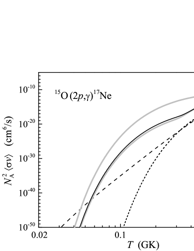
Figure 1: Reaction rate for ¹⁵O($2p$,$\gamma$)¹⁷Ne reaction. Solid curve shows calculations of this paper. Gray curves indicate boundaries due to uncertainties in the input (e.g. the upper gray curve is obtained with parameter set $\Gamma_{\gamma}^{\max}$ from Table 2). Dashed and dotted curves show full result from Ref. gor95 and resonance contribution to it respectively.

The results of rate calculations for this reaction are shown in Fig. 1 and in Table 1. They differ significantly from the results of Ref. gor95 (shown in Fig. 1 by dashed and dotted curves). For the temperature range of astrophysical interest ($\sim 0.3-3$ GK, see wie99 , for example) the expected increase of the rate, compared to Ref. gor95 , is up to 4 orders of the magnitude, while maximal possible increase is up to 9 orders of the magnitude.

The reasons of difference are evident from Table 2.

(i) The level scheme of ¹⁷Ne has been somewhat updated (see e.g. Ref. gui98 ) since the the work gor95 had been written.

(ii) The use of Eq. (15) includes the first $3/2^{-}$ excited state of ¹⁷Ne into treatment (it was omitted in Ref. gor95 , as there is no sequential capture path to this state). The important difference of the situation with this state from the others is that gamma width of this state is known to be much larger than the $2p$ width and the reaction rate Eq. (16) is entirely defined by the $2p$ width for the simultaneous two-proton emission. At the moment there exist two theoretical calculations of this width $\Gamma_{2p}=4.1\times 10^{-16}$ MeV gri03 , $\Gamma_{2p}=3.6\times 10^{-12}$ MeV gar04 , and a quite relaxed experimental lower lifetime limit of $\tau>26$ ps chr02 (which corresponds to the width $\Gamma_{2p}<2.5\times 10^{-11}$ MeV). Values $\Gamma_{2p}$ from Refs. gri03 and chr02 are used to estimate, respectively, the lower and the upper boundaries for the band of expected values of the rate (see Fig. 1). The resonance contribution of this state is dominating the rate in the temperature range $0.05-0.35$ GK if we take theoretical $2p$ width from Ref. gri03 , and up to 1.2 GK if we consider the experimental limit.

Table 1: Reaction rates multiplied by $N^{2}_{A}$ (in cm⁶/s) for ¹⁵O($2p$,$\gamma$)¹⁷Ne reaction.

$T$ (GK)	Ref. gor95	This work	This work upper
0.3	$2.9\times 10^{-23}$	$4.9\times 10^{-19}$	$2.9\times 10^{-14}$
0.5	$6.0\times 10^{-18}$	$2.1\times 10^{-15}$	$1.3\times 10^{-12}$
0.6	$1.2\times 10^{-16}$	$2.8\times 10^{-14}$	$2.8\times 10^{-12}$
0.8	$5.6\times 10^{-15}$	$6.3\times 10^{-13}$	$6.9\times 10^{-12}$
1.0	$5.0\times 10^{-14}$	$3.5\times 10^{-12}$	$1.3\times 10^{-11}$
1.5	$1.1\times 10^{-12}$	$2.5\times 10^{-11}$	$3.8\times 10^{-11}$
2.0	$6.0\times 10^{-12}$	$5.1\times 10^{-11}$	$6.8\times 10^{-11}$
3.0	$4.3\times 10^{-11}$	$7.6\times 10^{-11}$	$1.1\times 10^{-10}$
5.0	$2.5\times 10^{-10}$	$7.3\times 10^{-11}$	$2.3\times 10^{-10}$

(iii) In paper gor95 the gamma widths for ¹⁷Ne were taken from studied transitions in the isobaric mirror partner ¹⁷N. Recently the decay of the first excited states of ¹⁷Ne (3/2^-, 5/2^-) has been studied via intermediate energy Coulomb excitation of a radioactive ¹⁷Ne beam on a ¹⁹⁷Au target chr02 . In this paper the transition matrix elements $B($E2,$1/2^{-}\!\rightarrow 3/2^{-})$ and $B($E2,$1/2^{-}\!\rightarrow 5/2^{-})$ have been deduced. We use the deduced $B($E2$)$ value from Ref. chr02 to calculate the gamma width of the $5/2^{-}$ state. The result is shown in Table 2. This width appears to be about 30 times larger that the corresponding width of the mirror state in ¹⁷N. This is, probably, connected to the fact that at the proton-rich side the number of the protons contributing gamma transitions is larger and these protons are situated at larger distances compared with tightly bound protons in ¹⁷N. This situation is also expected for the other states in ¹⁷Ne (compared to the states in ¹⁷N), which is reflected by an order of the magnitude increase of the other widths for estimates of the upper limits (column $\Gamma_{\gamma}^{\max}$ in Table 2).

Table 2: Resonance parameters of ¹⁷Ne states used in the ¹⁵O($2p$,$\gamma$)¹⁷Ne reaction calculations. The column $\Gamma_{\gamma}^{\max}$ shows the upper experimental limit for $\Gamma_{\gamma}$ values, and $\Gamma_{\gamma}^{\min}$ the values used for lower limit estimates. The listed set of states is sufficient for rate calculations up to 5 GK. The widths and branchings, which are not specially discussed are from ajz88 .

State	Ref. gor95		This work
$J^{\pi}$	$E$ (keV)	$\Gamma_{\gamma}$ (eV)	$E$ (keV)	$\Gamma^{\min}_{\gamma}$ (eV)	$\Gamma_{\gamma}^{\max}$ (eV)
$3/2^{-}$			1288	$4.1\times 10^{-10}$	$2.5\times 10^{-5}$
$5/2^{-}$	1907	$6.0\times 10^{-5}$	1764	$1.7\times 10^{-3}$	$2.0\times 10^{-3}$
$1/2^{+}$	1850	$1.6\times 10^{-5}$	1908	$1.6\times 10^{-5}$	$2.1\times 10^{-4}$
$5/2^{+}$	2526	$2.0\times 10^{-5}$	2651	$9.0\times 10^{-6}$	$9.9\times 10^{-5}$
$3/2^{-}$	3204	$0.022$	3204	0.019	0.19

III.2 ¹⁸Ne($2p$,$\gamma$)²⁰Mg reaction

For the ¹⁸Ne($2p$,$\gamma$)²⁰Mg reaction there are no three-body states which were not taken into account in Ref. gor95 , so, no significant update of the rate is expected here. However, the level scheme and gamma widths are not known experimentally for this nucleus and this should be reflected in the rate calculations

Table 3: Resonance parameters of ²⁰Mg states used in the ¹⁸Ne($2p$,$\gamma$)²⁰Mg reaction calculations.

State	This work lower		This work upper
$J^{\pi}$	$E$ (keV)	$\Gamma_{\gamma}$ (eV)	$E$ (keV)	$\Gamma_{\gamma}$ (eV)
$4^{+}_{1}$	3570	$2.1\times 10^{-4}$	3451	$5.6\times 10^{-4}$
$2^{+}_{2}$	4072	$1.3\times 10^{-3}$	3857	$8.9\times 10^{-2}$
$0^{+}_{2}$	4456	$1.4\times 10^{-3}$	4317	$1.4\times 10^{-3}$
$4^{+}_{2}$	4850	$2.6\times 10^{-3}$	4699	$2.6\times 10^{-3}$
$2^{+}_{3}$	5234	$2.9\times 10^{-1}$	4978	$2.9\times 10^{-1}$

In the cases of $2p$ capture into ¹⁷Ne and ⁴⁰Ti the gamma widths from mirror isobaric partners were used in Ref. gor95 . In contrast, for capture into ²⁰Mg the systematics values were utilized. The theoretical $B$(E2) values for some low-lying states in ²⁰Mg have been calculated recently in Ref. des98 . The $B$(E2,$4^{+}_{1}\!\rightarrow 2^{+}_{1}$) was found to be 28.2 or 11.6 $e^{2}$fm⁴ (for V2 and MN forces respectively) and $B$(E2,$2^{+}_{2}\!\rightarrow 0^{+}_{1}$) was found to be 2.9 or 1.9 $e^{2}$fm⁴. These reduced probabilities give gamma widths $5.6\times 10^{-4}$ or $2.3\times 10^{-4}$ eV for $4^{+}_{1}$ state (which is comparable to value $2.1\times 10^{-4}$ eV used in gor95 ) and $2.0\times 10^{-3}$ or $1.3\times 10^{-3}$ eV for $2^{+}_{2}$ state (which is significantly less than $8.9\times 10^{-2}$ eV used in gor95 ). We combine the largest and the lowest gamma widths from Refs. gor95 and des98 to estimate the upper and the lower boundaries for the rate (see Table 3). To incorporate in this estimate the sensitivity to the level scheme we also use for the lower estimate the energies of the states from ²⁰O. The distance between levels here is expected to be somewhat larger than in ²⁰Mg gor95 and the reaction rate thus should further decrease.

Table 4: Reaction rates multiplied by $N^{2}_{A}$ (in cm⁶/s) for ¹⁸Ne($2p$,$\gamma$)²⁰Mg reaction.

$T$ (GK)	Ref. gor95	This work lower	This work upper
0.3	$4.4\times 10^{-21}$	$9.3\times 10^{-28}$	$2.5\times 10^{-25}$
0.5	$3.3\times 10^{-17}$	$4.3\times 10^{-20}$	$1.8\times 10^{-18}$
0.6	$4.8\times 10^{-16}$	$3.0\times 10^{-18}$	$8.3\times 10^{-17}$
0.8	$1.8\times 10^{-14}$	$5.1\times 10^{-16}$	$9.5\times 10^{-15}$
1.0	$2.4\times 10^{-13}$	$9.6\times 10^{-15}$	$1.8\times 10^{-13}$
1.5	$6.8\times 10^{-12}$	$3.7\times 10^{-13}$	$1.1\times 10^{-11}$
2.0	$9.7\times 10^{-11}$	$2.0\times 10^{-12}$	$8.0\times 10^{-11}$
3.0	$4.8\times 10^{-10}$	$1.5\times 10^{-11}$	$4.4\times 10^{-10}$
5.0	$2.4\times 10^{-9}$	$1.4\times 10^{-10}$	$1.2\times 10^{-9}$

The results of calculations are shown in Table 4. The upper boundary in our calculations is in a good agreement with results of gor95 (factor of two) at $T\geq 0.8$ GK. It was shown in gor95 that below 0.8 GK the nonresonant contribution to the reaction rate dominates, which explains the discrepancy in Table 4 at low temperatures.

III.3 ³⁸Ca($2p$,$\gamma$)⁴⁰Ti reaction

For the ³⁸Ca($2p$,$\gamma$)⁴⁰Ti reaction one three-body state was omitted in Ref. gor95 . According to the isobaric symmetry there should be a $0^{+}_{2}$ state located at about 2.121 MeV excitation energy. The two-proton separation energy used in Ref. gor95 is $S_{2p}=1.582$ MeV. Another estimate (e.g. nndc ) is $S_{2p}=1.370$ MeV. In the first case the $2p$ emission energy for $0^{+}_{2}$ state is 539 keV and (following Refs. gri03a ; gri03b ) the two-proton width can be estimated as about $10^{-21}$ MeV. In the second case the $2p$ energy is 751 keV and the estimated two-proton width is around $10^{-18}$ MeV. For other states we use parameters from Ref. gor95 (see Table 5), which mainly come from the isobaric mirror partner ⁴⁰Ar. To estimate the upper boundary for the reaction rate we increase the gamma widths of $4^{+}_{1}$ and $2^{+}_{3}$ states by an order of the magnitude. As we have already discussed, one could expect a significant increase of the gamma widths when we come to the proton-rich mirror partner. To estimate the sensitivity to the level scheme (which is not known for ⁴⁰Ti) we use the smaller $2p$ separation energy $S_{2p}=1.370$ MeV for the estimate of the lower boundary and $S_{2p}=1.582$ MeV for the upper boundary. Again, as in the case of ²⁰Mg, the increase of the state energy above $2p$ threshold leads to decrease of the corresponding reaction rate. For that reason we use the larger $2p$ width for estimate of the lower boundary (Table 5, line 1). The larger two proton width corresponds to the case of larger energy of states above $2p$ separation threshold.

Table 5: Resonance parameters of ⁴⁰Ti states used in the ³⁸Ca($2p$,$\gamma$)⁴⁰Ti reaction calculations. In the “Type” column the type of width is specified, which defines the contribution of the state to reaction rate. The “Lower” set of widths is used in the calculations with $S_{2p}=1.370$ MeV, while the “Upper” set with $S_{2p}=1.582$ MeV.

$J^{\pi}$	$E$ (keV)	Type	“Lower” $\Gamma$ (eV)	“Upper” $\Gamma$ (eV)
$0^{+}_{2}$	2121	$\Gamma_{2p}$	$10^{-12}$	$10^{-15}$
$2^{+}_{2}$	2524	$\Gamma_{p}$	$1.0\times 10^{-5}$	$1.0\times 10^{-5}$
$4^{+}_{1}$	2892	$\Gamma_{\gamma}$	$2.0\times 10^{-4}$	$2.0\times 10^{-3}$
$2^{+}_{3}$	3208	$\Gamma_{\gamma}$	$1.0\times 10^{-2}$	$1.0\times 10^{-1}$

The results of calculations for ³⁸Ca($2p$,$\gamma$)⁴⁰Ti are given in Fig. 2 and Table 6. Our results are somewhat larger (1–2 orders of magnitude) than results of gor95 for temperatures $T>1$ GK. They more or less overlaps at lower temperatures. The effect of inclusion of $0^{+}_{2}$ 2.121 MeV state can be seen in Fig. 2: the range between upper and lower boundaries shrinks at $T<0.35$ GK. This happens because the contribution of the $0^{+}_{2}$ state is much larger in the “Lower” parameter set, which otherwise provides a smaller reaction rate.

Table 6: Reaction rates multiplied by $N^{2}_{A}$ (in cm⁶/s) for ³⁸Ca($2p$,$\gamma$)⁴⁰Ti reaction.

$T$ (GK)	Ref. gor95	This work lower	This work upper
0.3	$2.1\times 10^{-25}$	$7.0\times 10^{-28}$	$2.3\times 10^{-24}$
0.5	$1.0\times 10^{-19}$	$7.8\times 10^{-21}$	$1.1\times 10^{-18}$
0.6	$2.4\times 10^{-18}$	$4.0\times 10^{-19}$	$3.1\times 10^{-17}$
0.8	$1.1\times 10^{-16}$	$5.3\times 10^{-17}$	$3.0\times 10^{-15}$
1.0	$1.3\times 10^{-15}$	$1.2\times 10^{-15}$	$7.1\times 10^{-14}$
1.5	$7.0\times 10^{-14}$	$1.3\times 10^{-13}$	$6.0\times 10^{-12}$
2.0	$5.2\times 10^{-13}$	$1.5\times 10^{-12}$	$5.1\times 10^{-11}$
3.0	$3.0\times 10^{-12}$	$1.4\times 10^{-11}$	$3.2\times 10^{-10}$
5.0	$8.0\times 10^{-12}$	$5.0\times 10^{-11}$	$8.2\times 10^{-10}$

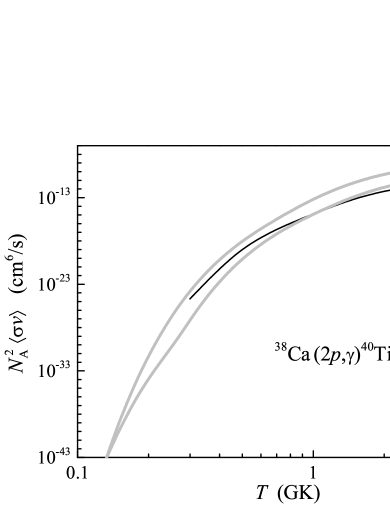
Figure 2: Reaction rate for ³⁸Ca($2p$,$\gamma$)⁴⁰Ti reaction. Solid curve shows the result from gor95 . Gray curves indicate upper and lower boundaries for our results (see Table 6) due to existing uncertainties in the input.

III.4 ⁴He($n\alpha$,$\gamma$)⁹Be reaction

The stellar reaction rate for ⁴He($n\alpha$,$\gamma$)⁹Be process has been studied several times in the recent years fow75 ; cau88 ; gor95a ; efr98 ; ang99 ; buc01 . The results are in overall agreement, except for the latest paper buc01 . In this work the rate is obtained which is significantly higher (for temperatures $T>3$ GK) than the rates in the previous studies.

In our studies here we have found that the sequential formalism underestimate the reaction rate only if the width of the state for direct decay into continuum is dominating (see Section II.1). The low-lying ($E\leq 3$ MeV) ⁹Be states typically have strong ⁸Be+$n$ decay branchings. Only the $5/2^{-}$ 2.429 MeV state is an exception: the branching to the three-body channel is $93-95\%$ ajz88 . The gamma width of this state is 0.091 eV ajz88 . The results of our calculations are shown in Fig. 3 and Table 7. In these calculations we use a version of Eq. (16) without an assumption about narrow widths of the resonances and the capture cross section is parametrized as in Ref. ang99 (with exception that $5/2^{-}$ state is included). The results obtained are in a very good agreement with ang99 . The increase of the rate due to addition of the $5/2^{-}$ state is $11\%$ at most in the temperature range up to 10 GK. This small change is connected with comparatively small gamma width of this state: the gamma widths of the other states in the capture cross section parametrization used in ang99 are around $0.45-0.9$ eV. So, the uncertainty of the reaction rate due to uncertainties of the experimental data found in ang99 is significantly larger than correction connected with $5/2^{-}$ state (see Table 7).

The mentioned experimental uncertainty could be even larger than it was inferred in Ref. ang99 . The analysis, provided in Ref. efr98 in the framework of the semimicroscopic model, demonstrated that the older photodisintegration data for ⁹Be ham53 ; gib59 ; joh62 could be more preferable than the more up-to-date results fui82 (on which, e.g. the parametrization of the cross section used in Ref. ang99 is based). The reaction rate found in paper efr98 (as well as in the early work fow75 ) is around $35\%$ larger than the rate in Ref. ang99 .

Figure 3: Reaction rate for ⁴He($n\alpha$,$\gamma$)⁹Be reaction. The solid curve shows our result (see also Table 7). The dashed curve is the same, but without $5/2^{-}$ 2.429 MeV state contribution (this coincides with result of Ref. ang99 ). The dash-dotted curve is contribution from the near threshold $1/2^{+}$ state. The dotted curve shows calculations Ref. buc01 .

Paper buc01 is generally dedicated to the R-matrix analysis of the $\beta$-delayed particle decay of ⁹C via the excited states in ⁹B. The authors utilize the R-matrix parameters obtained in the decay studies of ⁹B for the caption calculations in ⁹Be. The reaction rate calculated in this work is consistent with the other results at low temperatures, but is qualitatively different at $T>3$ GK (see Fig. 3, dotted curve). The rise of the reaction rate at higher temperatures is connected, according to buc01 , with contribution of sequential capture of $\alpha$-particle on the broad ground state of ⁵He. Such capture path has never been considered elsewhere. It should be noted that in the framework of sequential formalism this is a valid question: how narrow should be the intermediate state, to be considered within this formalism. Really, the sequential formalism is evidently correct in the limit of infinitely narrow intermediate state. However, in the other limit (an infinitely broad state), we have just nonresonant continuum and the sequential formalism should fail at some point. This issue is qualitatively discussed in Section II.3. Our work resolve this question in a very natural way: we state that contributions of different sequential and three-body channels should add up in a way, which makes their relative contributions unimportant. So, inclusion of capture via ⁵He into formalism should not lead to any significant changes (compared to conventional sequential capture via ⁸Be g.s.), until there exist states with dominating three-body decay branch (which is not accounted in sequential formalism) and large gamma widths. No such states are known in the energy range of interest. The reaction rate from Ref. buc01 can be reproduced within our formalism only if we assume the gamma width for the 3 MeV state in ⁹Be to be about 15 eV and also assume one more state at about 5 MeV with gamma width above 1 keV. Such assumptions are quite unrealistic.

Unfortunately, there is an evidence for problems in Ref. buc01 , which probably have leaded to the discussed strange result. In Eq. (32) of this work the penetrability is present in the first power, while it should be in the second (as we speak about elastic cross section). Possibly this is the reason of the qualitatively incorrect behaviour of the intermediate population values (see Fig. 8 in Ref. buc01 ). For example, the population $\langle\sigma(E)v/\Gamma(E)\rangle$ for ⁵He g.s. should decrease as $T$ at low temperature. In Fig. 8 of Ref. buc01 this value has a rapid rise at low temperature. Using Eq. (32) from Ref. buc01 “as is” one gets behaviour $T^{-1/2}$ at low $T$ in agreement with this figure.

Table 7: Reaction rates multiplied by $N^{2}_{A}$ (in cm⁶/s) for ⁴He($n\alpha$,$\gamma$)⁹Be reaction.

$T$ (GK)	Ref. ang99	Ref. ang99 upper	This work
2	$1.80\times 10^{-7}$	$2.20\times 10^{-7}$	$1.83\times 10^{-7}$
4	$5.48\times 10^{-8}$	$6.99\times 10^{-8}$	$5.94\times 10^{-8}$
6	$2.88\times 10^{-8}$	$3.83\times 10^{-8}$	$3.20\times 10^{-8}$
8	$1.81\times 10^{-8}$	$2.47\times 10^{-8}$	$2.02\times 10^{-8}$
10	$1.23\times 10^{-8}$	$1.70\times 10^{-8}$	$1.36\times 10^{-8}$

So, the difference of our approach found in the case of ⁴He($n\alpha$,$\gamma$)⁹Be reaction is not significant. It is much smaller than the other uncertainties (see Refs. efr98 and ang99 ). However, our formalism excludes such a possibility as an importance of broad intermediate ⁵He state buc01 .

IV Conclusion

We use the formalism based on the S-matrix for $3\rightarrow 3$ scattering to derive the reaction rate for the three-body resonant radiative capture. This derivation makes especially evident that (i) all the three-body states should be included in the treatment (even if there is no opportunity of a sequential capture to the state), (ii) the detailed knowledge of the intermediate states is unnecessary to calculate the resonant rates and (iii) only the knowledge of particle and gamma widths for the three-body states is needed to calculate the resonant rates (not the relative contribution of direct and sequential mechanisms).

This formalism, together with the modern results on $2p$ and $\gamma$ widths of ¹⁷Ne states, allows us to update significantly the capture rate for the ¹⁵O($2p$,$\gamma$)¹⁷Ne reaction. The updated rate is up to 4–9 orders of the magnitude larger (in the temperature range of astrophysical interest). The experimental derivation of the $2p$ width of the first excited state in ¹⁷Ne is found to be very important for refining this rate. The ³⁸Ca($2p$,$\gamma$)⁴⁰Ti reaction rate has also got a considerable increase. Thus the conclusions about importance of the $2p$ capture reactions could possibly be more optimistic than in Ref. gor95 . We also discuss the impact of our approach on the ¹⁸Ne($2p$,$\gamma$)²⁰Mg, and ⁴He($n\alpha$,$\gamma$)⁹Be reaction rates. Our studies emphasize the importance of better gamma width information for $2p$ capture rates (experimental or theoretical, if the first is not available).

The studies of this work are restricted to resonant reactions (and correspondingly to relatively high temperatures). We are planning to perform accurate three-body studies of the nonresonant contributions in the forthcoming paper.

- (1) J. Görres, M. Wiescher, and F.-K. Thielemann, Phys. Rev. C 51, 392 (1995).
- (2) S. E. Woosely et al., Astrophys. J. 433, 229 (1994).
- (3) K. Takahashi, J. Witti, and H. T. Janka, Astron. Astrophys. 286, 857 (1994).
- (4) W. A. Fowler, G. R. Caughlan, and B. A. Zimmerman, Annu. Rev. Astron. Astrophys. 13, 69 (1975).
- (5) G. R. Caughlan, and W. A. Fowler, At. Data Nucl. Data Tables 40, 283 (1988).
- (6) J. Görres, H. Herndl, I. J. Thompson, and M. Wiescher, Phys. Rev. C 52, 2231 (1995).
- (7) V. D. Efros, H. Oberhummer, A. Pushkin, and I. J. Thompson, Eur. Phys. J. A 1, 447 (1998).
- (8) C. Angulo et al., Nucl. Phys. A656, 3 (1999).
- (9) L. Buchmann, E. Gete, J. C. Chow, J. D. King, and D. F. Measday, Phys. Rev. C 63, 034303 (2001).
- (10) V. I. Goldansky, Nucl. Phys. 19, 482 (1960).
- (11) L. V. Grigorenko, R. C. Johnson, I. G. Mukha, I. J. Thompson, and M. V. Zhukov, Phys. Rev. Lett. 85, 22 (2000).
- (12) L. V. Grigorenko, R. C. Johnson, I. G. Mukha, I. J. Thompson, and M. V. Zhukov, Phys. Rev. C 64, 054002 (2001).
- (13) L. V. Grigorenko, I. G. Mukha, I. J. Thompson, and M. V. Zhukov, Phys. Rev. Lett. 88, 042502 (2002).
- (14) M. Pfützner, et al., Eur. Phys. J. A 14, 279 (2002).
- (15) J. Giovinazzo, et al., Phys. Rev. Lett. 89, 102501 (2002).
- (16) M. J. Chromik et al., Phys. Rev. C 66, 024313 (2002).
- (17) L. V. Grigorenko, I. G. Mukha, and M. V. Zhukov, Nucl. Phys. A713, 372 (2003); erratum, Nucl. Phys. A, in print.
- (18) L. V. Grigorenko, I. G. Mukha, and M. V. Zhukov, Nucl. Phys. A714, 425 (2003).
- (19) B. A. Brown and F. C. Barker, Phys. Rev. C 67, 041304(R) (2003).
- (20) L. V. Grigorenko and M. V. Zhukov, Phys. Rev. C 68, 054005 (2003).
- (21) E. Garrido, D. V. Fedorov, and A. S. Jensen, Nucl. Phys. A733, 85 (2004).
- (22) W. A. Fowler, G. R. Caughlan, and B. A. Zimmerman, Annu. Rev. Astron. Astrophys. 5, 525 (1967).
- (23) K. Nomoto, F. Thielemann, and S. Miyaji, Astron. Astrophys. 149, 239 (1985).
- (24) A. I. Baz’, S. P. Merkuriev, Theor. Math. Phys. 31, 48 (1977).
- (25) S. P. Merkuriev, L. D. Faddeev, “Quantum scattering theory for few particle systems”, Moscow, Publishing House “Science”, Main Editorial Office for Physical and Mathematical Literature, 1985 (in Russian).
- (26) F. Ajzenberg-Selove, Nucl. Phys. A490, 1 (1988).
- (27) G. Nyman et al., Nucl. Phys. A510, 189 (1990).
- (28) M. Wiescher, J. Görres, and H. Schatz, J. Phys. G: Nucl. Part. Phys. 25, R133 (1999).
- (29) V. Guimarães et al., Phys. Rev. C 58, 116 (1998).
- (30) P. Descouvemont, Phys. Lett. B437, 7 (1998).
- (31) NNDC database, http://www.nndc.bnl.gov
- (32) B. Hammermesh, and C. Kimball, Phys. Rev. 90, 1063 (1953).
- (33) J. H. Gibbons, R. L. Maclin, J. B. Marion, and H. W. Schmitt, Phys. Rev. 114, 1319 (1959).
- (34) W. John, and J. M. Prosser, Phys. Rev. 127, 231 (1962).
- (35) M. Fuishiro, K. Okamoto, and T. Tsuimoto, Can. J. Phys. 60, 1672 (1982).