Long-wavelength spin- and spin-isospin correlations in nucleon matter

Abstract

We analyse the long-wavelength response of a normal Fermi liquid using Landau theory. We consider contributions from intermediate states containing one additional quasiparticle-quasihole pair as well as those from states containing two or more additional quasiparticle-quasihole pairs. For the response of an operator corresponding to a conserved quantity, we show that the behavior of matrix elements to states with more than one additional quasiparticle-quasihole pair at low excitation energies $\omega$ varies as $1/\omega$. It is shown how rates of processes involving transitions to two quasiparticle-quasihole states may be calculated in terms of the collision integral in the Landau transport equation for quasiparticles.

I Introduction

In liquid helium 3, the prototypical Fermi liquid, interactions between atoms are to a very good approximation invariant under independent rotations in coordinate space and in spin space. This fact, together with the translational invariance of the system, makes for an economical description of the properties of the system in terms of Landau’s theory of normal Fermi liquids. The reason for this is that at long wavelengths, the only excitations of importance for the low-frequency response are those with an added quasiparticle-quasihole pair, and collective modes such as zero sound, which are coherent superpositions of single quasiparticle-quasihole pairs. An analysis of the behavior of matrix elements of the long-wavelength components of the density operator to single-pair and multipair states was given by Pines and Nozières pines , and our purpose in this paper is to extend the analysis to more general responses.

From investigations of the response to probes more general than a scalar potential leggett ; bp , it is clear that conservation laws play a key role in determining the form of long-wavelength matrix elements of an operator. In nuclear matter, interactions are not central, due to the large tensor contribution coming from exchange of pions and to other terms that give rise to spin-orbit coupling. As a consequence, the total spin is not a conserved quantity and matrix elements to states containing more than one quasiparticle-quasihole pair (which we shall in future refer to simply as a pair) do not vanish at long wavelengths. A qualitative discussion of the effects of noncentral interactions is given in Ref. op and Landau theory was extended to take into account noncentral interactions in Ref. ohp .

Multipair states play an important role in the context of neutrino processes in dense matter. The rates of a variety of weak interaction processes can be expressed in terms of correlation functions for nucleons or other constituents raffelt1 . The reason for this simplification is that, due to the interactions between leptons and hadrons being due to weak and electromagnetic effects, rates may be expressed as a convolution of a hadronic correlation function and a leptonic one. Because correlations among leptons are relatively weak, the most difficult part of calculating weak interaction processes in dense matter is the evaluation of the hadronic correlation functions. A review of calculations of rates may be found in Ref. prakash . Processes such as bremsstrahlung of neutrino-antineutrino pairs in nucleon-nucleon interactions and the production of neutrinos and antineutrinos by the modified Urca process are both intrinsically two quasiparticle, two quasihole processes, and they are important when the corresponding single-pair process is kinematically forbidden. Bremsstrahlung by creation of a single nucleon pair is kinematically forbidden, since the velocity of a quasiparticle is always less than $c$, and the direct Urca process, the single nucleon pair analog of the modified Urca process, is allowed in dense matter only for certain compositions. There are many calculations of rate of scattering of neutrinos by nucleons that take into account single-pair processes chris1 ; reddy but, as Raffelt and collaborators have stressed raffelt2 , multipair processes can be important quantitatively.

The purpose of this paper is to express the two-quasiparticle-quasihole contribution to the response in terms of the collision integral in the Landau kinetic equation for quasiparticles. Landau theory provides a clear separation between long-wavelength degrees of freedom, which are treated explicitly, and short-wavelength ones whose effects are included through the use of parameters that include the effects of renormalization of matrix elements of currents and interparticle interactions. Another strength of the Landau theory is that it brings out clearly the role played by conservation laws. For simplicity, we shall restrict ourselves to normal systems and we shall not consider effects of nucleon pairing and superfluidity.

II Basic formalism

In Landau theory, one limits oneself to temperatures low compared with the Fermi temperatures of the constituents and regards the elementary excitations as being quasiparticles which may be characterized by an effective mass $m^{*}_{i}$, where the index $i={\rm n},{\rm p}$ denotes neutrons and protons, respectively. We shall treat the nucleons as nonrelativistic, which is a good first approximation.

If a system is subjected to a perturbation

$$H^{\prime}={\cal O}_{\bf q}U_{\bf q}e^{-i\omega t}+{\rm Hermitean\ conjugate},$$ (1)

the Fourier transform of the linear response of the expectation value of the operator ${\cal O}_{\bf q}$ at frequency $\omega$ is given for a system invariant under parity by pines

$$<{\cal O}_{\bf q}>_{\omega}=-\chi(q,\omega)U_{\bf q},$$ (2)

where the linear response function is defined by

$$\chi(q,\omega)=\sum_{jl}\frac{{\rm e}^{-E_{l}/T}}{Z}|({{\cal O}_{\bf q}^{\dagger}})_{jl}|^{2}\frac{2\omega_{jl}}{{\omega}_{jl}^{2}-(\omega+i\eta)^{2}}.$$ (3)

Here $l$ denotes an initial state, $j$ denotes an intermediate state and $\omega_{jl}=E_{j}-E_{l}$, where $E_{j}$ and $E_{l}$ are the energies of the states, $Z=\sum_{j}{\rm e}^{-E_{j}/T}$ is the partition function and $T$ is the temperature. In this paper we shall only consider the response of the physical quantity which is coupled to the applied field. For systems with noncentral interactions, there are generally off-diagonal terms, such as the response of the spin in the $x$ direction when a magnetic field is applied in the $z$ direction. Since such effects vanish in the limit of small $q$, they are generally of less importance than the diagonal response chris1 .

A particularly useful quantity related to this is the dynamical structure factor, which is defined by

$$S_{\cal O}(q,\omega)=\frac{1}{Z}\sum_{jl}{\rm e}^{-E_{l}/T}|({{\cal O}_{\bf q}^{\dagger}})_{jl}|^{2}\delta(\omega-\omega_{jl})$$

$$=\frac{1}{\pi(1-{\rm e}^{-\omega/T})}{\rm Im}\chi(q,\omega).$$ (4)

To make explicit calculations we shall use the language of diagrammatic many-body theory expressed in terms of fully renormalized nucleon propagator $G({\bf p},\omega)$, where $\bf p$ is the particle momentum and $\omega$ its energy. For simplicity we shall not write out spin and isospin labels except where necessary for clarity. We shall further write the propagator as the sum of a coherent part, which corresponds to a single quasiparticle or quasihole, and an incoherent part, which takes into account more complicated intermediate states:

$$G(p,\omega)=G^{\rm coh}(p,\omega)+G^{\rm inc}(p,\omega),$$ (5)

where the coherent part has the form

$$G^{\rm coh}(p,\omega)=\frac{z_{p}}{\omega-\epsilon_{p}+i\eta}.$$ (6)

Here $\epsilon_{p}$ is the quasiparticle energy, measured with respect to the chemical potential for the species in question and $z_{p}$ is the wave function renormalization factor.

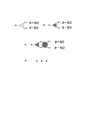
Figure 1: Diagrams for the matrix element for a transition to a state with one quasiparticle-quasihole pair. The dashed line represents the interaction with the applied external field. The open circle corresponds to the sum of all connected diagrams, and the shaded ones to all connected diagrams irreducible with respect to a single quasiparticle-quasihole pair.

III Single-pair processes

To set the scene and establish notation, we consider transitions to states with a single quasiparticle-quasihole pair. The matrix element for the process is indicated diagrammatically in Fig. 1 by the open circle. In Fig. 1 the single particle propagator represent only the coherent part. By the standard techniques of microscopic many-body theory nozieres , this may be expressed in terms of diagrams irreducible with respect to states having a single quasiparticle-quasihole pair in the channel with total momentum $\bf q$ as shown in the figure, where the hatched vertices correspond to the irreducible diagams. Algebraically, it is given in a compact matrix notation by

$${\cal O}_{\bf q}^{\rm sp}=\Lambda^{\cal O}z(1+\chi f)^{-1}\equiv\lambda^{\cal O},$$ (7)

where we suppress sums over momenta and particle species Here $\Lambda$ is the irreducible vertex for interaction with the external field,

$$\chi_{\bf p}({\bf q},\omega)=\frac{n_{\bf p+q/2}-n_{\bf p-q/2}}{\omega-\epsilon_{\bf p+q/2}+\epsilon_{\bf p-q/2}},$$ (8)

and

$$f_{\bf pp^{\prime}}=z_{p}z_{p^{\prime}}\Gamma^{\rm irr}({\bf p,p^{\prime}})$$ (9)

is the Landau quasiparticle interaction, $\Gamma^{\rm irr}$ being the two-particle vertex function irreducible in the sense described above. We will give expressions for $\lambda^{\cal O}$ in the Appendix. For the long-wavelength, low-frequency response the only quasiparticles of importance are those to the Fermi surface, and we denote $z_{p_{\rm F}}$ by $z$. In the phenomenological theory, the quantity $g^{\cal O}\equiv z\Lambda^{\cal O}$ corresponds to an effective “charge” of a quasiparticle for the particular probe in question; for example in the case of a scalar probe, it is the total particle number carried by a quasiparticle and for a magnetic field it corresponds to the magnetic moment of the quasiparticle. For simplicity we have not written spin and isospin indices explicitly.

The contribution to the imaginary part of the response function is therefore

$${\rm Im}\chi^{\rm sp} = \pi\sum_{\bf p,spin}|{\cal O}_{\bf q}^{\rm sp}|^{2}(n_{\bf p+q/2}-n_{\bf p-q/2})\times$$ (10)

$$\delta(\omega-\epsilon_{\bf p+q/2}+\epsilon_{\bf p-q/2})$$

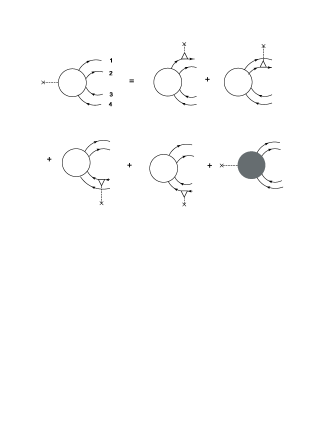
Figure 2: Diagrams for the matrix element for a transition to a state with two quasiparticle-quasihole pairs. As in Figure 1, open circles denote the sum of all connected diagrams, and here the hatched circle corresponds to the sum of all diagrams that do not have the external field attached to one of the external lines.

IV Two-pair processes

We turn now to intermediate states with two quasiparticles and two quasiholes. The matrix element for the process is illustrated in Fig. 2. Of particular interest to us are contributions in which the external field interacts directly with just one of the quasiparticles or quasiholes in the intermediate state. These are represented by the first four diagrams on the right hand side of the equation in Fig. 2, and they are particularly important for the response to operators which do not correspond to conserved quantities. As we shall see, they lead to divergences of matrix elements for low $\omega$ analogous to those found for bremsstrahlung. The corresponding effects in low-order perturbation theory have previously been drawn attention to in Ref. raffelt2 . The final term in Fig. 2 represents the remainder. We denote the quasiparticles and quasiholes in the intermediate state by the indices $i=1,\ldots,4$, as indicated. In this paper we shall consider only operators which do not convert neutrons into protons, or vice versa, that is they couple only to the third component of the isospin. When the operator can change the isospin, which is the case for the response function of interest for the modified Urca process, the situation is more complicated, and we shall comment on this point in the Conclusion.

For small $\bf q$, the contribution to the on-shell matrix element coming from the first term may be evaluated straightforwardly, and it is given by

$${\cal O}_{\bf q}^{\rm tp}=-z^{2}\Gamma\frac{1}{\omega-\epsilon_{{\bf p}_{1}}+\epsilon_{{\bf p}_{1}-{\bf q}}}\lambda^{\cal O}_{1}$$

$$\approx-{\cal A}\frac{\lambda^{\cal O}_{1}}{\omega-{\bf v_{\rm{}_{1}}\cdot q}},$$ (11)

where

$${\cal A}=z^{2}\Gamma$$ (12)

is the scattering matrix for two-quasiparticle scattering. Therefore the contribution to the matrix element from the first four terms is

$${\cal O}_{\bf q}^{\rm tp}=-{\cal A}\frac{1}{\omega}\left[\xi^{\cal O}_{1}+\xi^{\cal O}_{2}-\xi^{\cal O}_{3}-\xi^{\cal O}_{4}\right],$$ (13)

where

$$\xi^{\cal O}_{i}=\frac{\lambda^{\cal O}_{i}}{1-{\bf v_{\rm{}_{i}}\cdot q}/\omega}.$$ (14)

The imaginary part of the two-pair contribution to the response function is therefore

$${\rm Im}\chi^{\rm tp}=\frac{\pi}{4}\sum_{1234}\left\{|{\cal O}_{\bf q}^{\rm tp}|^{2}\times\right.$$

$$\left[n_{1}n_{2}(1-n_{3})(1-n_{4})-(1-n_{1})(1-n_{2})n_{3}n_{4}\right]\times$$

$$\left.\delta(\omega+\epsilon_{1}+\epsilon_{2}-\epsilon_{3}-\epsilon_{4})\delta({\bf q+p_{1}+p_{2}-p_{3}-p_{4}})\right\}.$$

where sums over quasiparticle states include sums over spins and isospins and the factor of $1/4$ is necessary to avoid overcounting. Inserting the expression (13), one finds traces

$${\rm Im}\chi^{\rm tp}=\pi\!\sum_{1234}\!\!\left\{|{\cal A}|^{2}\left(\frac{1}{\omega^{2}}\xi^{\cal O}_{1}\right)^{\scriptstyle*}\!\!\!\left(\xi^{\cal O}_{1}+\xi^{\cal O}_{2}-\xi^{\cal O}_{3}-\xi^{\cal O}_{4})\right)\right.\times$$

$$\left[n_{1}n_{2}(1-n_{3})(1-n_{4})-(1-n_{1})(1-n_{2})n_{3}n_{4}\right]\times$$

$$\left.\delta(\omega+\epsilon_{1}+\epsilon_{2}-\epsilon_{3}-\epsilon_{4})\delta({\bf q+p_{1}+p_{2}-p_{3}-p_{4}})\frac{}{}\right\}$$

(16)

Let us now consider the limit $\omega>>v_{\rm F}q$. For external fields that are independent of the particle momentum, the quantities $\lambda$ are independent of the direction of the quasiparticle momentum. For long-wavelength probes, the $\bf q$ in the momentum conservation condition may be ignored to leading order, and therefore Eq. (16) becomes

$${\rm Im}\chi^{\rm tp}=\frac{\pi}{\omega^{2}}\sum_{1234}\left\{|{\cal A}|^{2}\xi^{\cal O}_{1}(\xi^{\cal O}_{1}+\xi^{\cal O}_{2}-\xi^{\cal O}_{3}-\xi^{\cal O}_{4})\right.\times$$

$$\left[n_{1}n_{2}(1-n_{3})(1-n_{4})-(1-n_{1})(1-n_{2})n_{3}n_{4}\right]\times$$

$$\left.\delta(\omega+\epsilon_{1}+\epsilon_{2}-\epsilon_{3}-\epsilon_{4})\delta({\bf p_{1}+p_{2}-p_{3}-p_{4}})\right\}$$

(17)

For convenience, we adopt the usual convention that the phase of single-particle states is chosen so that $\lambda^{\cal O}$ is real.

It is instructive to rewrite this expression to show that the quantity that enters is very closely related to quasiparticle relaxation time. The collision term for two-quasiparticle scattering is given by

$$\frac{\partial n_{1}}{\partial t}=-\sum_{234}\left\{|{\cal A}|^{2}\right.\times$$

$$\left[n_{1}n_{2}(1-n_{3})(1-n_{4})-(1-n_{1})(1-n_{2})n_{3}n_{4}\right]\times$$

$$\left.\delta(\omega+\epsilon_{1}+\epsilon_{2}-\epsilon_{3}-\epsilon_{4})\delta({\bf p_{1}+p_{2}-p_{3}-p_{4}})\right\},$$ (18)

where in this equation the distribution function is not necessarily the equilibrium one. On linearizing this equation about the equilibrium distribution for quasiparticles with momentum $\bf p_{1}$, one finds

$$\frac{\partial n_{1}}{\partial t}=-\frac{\delta n_{1}}{\tau_{1}}$$ (19)

where

$$\frac{1}{\tau_{1}}=2\pi\sum_{234}\left\{|{\cal A}|^{2}[n_{2}(1-n_{3})(1-n_{4})+(1-n_{2})n_{3}n_{4}]\right.\!\!\times$$

$$\left.\delta(\omega+\epsilon_{1}+\epsilon_{2}-\epsilon_{3}-\epsilon_{4})\delta({\bf p_{1}+p_{2}-p_{3}-p_{4}})\right\}.$$ (20)

We now rewrite Eq. (17) so that the combinations of distribution functions is similar to that in Eq. (20). By virtue of the relationship

$$n(\epsilon)={\rm e}^{-\epsilon/T}[1-n(\epsilon)]$$ (21)

we may write

$$[n_{1}n_{2}(1-n_{3})(1-n_{4})-(1-n_{1})(1-n_{2})n_{3}n_{4}]\times$$

$$\delta(\omega+\epsilon_{1}+\epsilon_{2}-\epsilon_{3}-\epsilon_{4})=$$

$$\left[n_{1}-n(\epsilon_{1}+\omega)][n_{2}(1-n_{3})(1-n_{4})+(1-n_{2})n_{3}n_{4}\right]\times$$

$$\delta(\omega+\epsilon_{1}+\epsilon_{2}-\epsilon_{3}-\epsilon_{4}),$$

from which it follows that we may rewrite Eq. (17) as

$${\rm Im}\chi^{\rm tp}=\frac{1}{2\omega^{2}}\sum_{1}(\lambda^{\cal O}_{1})^{2}\frac{[n_{1}-n(\epsilon_{1}+\omega)]}{\tau^{\cal O}_{1}(\epsilon_{1}+\omega)}$$ (23)

where

$$\frac{1}{\tau^{\cal O}_{1}(\epsilon_{1}+\omega)}=2\pi\sum_{234}\left\{|{\cal A}|^{2}\left[1+\frac{\lambda^{\cal O}_{2}-\lambda^{\cal O}_{3}-\lambda^{\cal O}_{4}}{\lambda^{\cal O}_{1}}\right]\right.\times$$

$$\left[n_{2}(1-n_{3})(1-n_{4})+(1-n_{2})n_{3}n_{4}\right]\times$$

$$\left.\frac{}{}\!\!\delta(\omega+\epsilon_{1}+\epsilon_{2}-\epsilon_{3}-\epsilon_{4})\delta({\bf q+p_{1}+p_{2}-p_{3}-p_{4}})\right\}$$

(24)

is the relaxation rate for the quantity $\lambda^{\cal O}$ for a system close to equilibrium. This gives the collision rate weighted by the change in $\lambda$ of all the quasiparticles in a collision.

Depending on the properties of the operator $\cal O$, the matrix elements to two pair states can have different sorts of behavior. Let us begin by considering the limit $\omega\gg v_{\rm F}q$, where $v_{\rm F}$ is a typical Fermi velocity. The matrix element then becomes proportional to $[\lambda^{\cal O}({\bf p}_{1})+\lambda^{\cal O}({\bf p}_{2})-\lambda^{\cal O}({\bf p}_{3})-\lambda^{\cal O}({\bf p}_{4})]/\omega$. If the operator $\cal O$ is the particle density, $\lambda^{\cal O}$ becomes a constant at for $\omega\gg v_{\rm F}q$. Since the interaction conserves particle number, it also conserves the number of quasiparticles and therefore in this limit, $\lambda^{\cal O}({\bf p}_{1})+\lambda^{\cal O}({\bf p}_{2})-\lambda^{\cal O}({\bf p}_{3})-\lambda^{\cal O}({\bf p}_{4})$ vanishes. It the operator is that for a component of the spin, a similar argument will apply if the interactions between components are central, that is their spin structure of the form of the unit operator or of the spin-exchange operator. However, when there are non-central interactions, e.g. spin-orbit or tensor forces, the combination of $\lambda$’s will not generally vanish. For example, two quasiparticles with spin up can scatter to states with two quasiparticles with spin down, in which case the matrix element to a two-pair state will diverge as $1/\omega$. For the operator for the number density of particles, the leading contribution to the matrix element for a transition to a two-pair state will have a factor $v_{\rm F}q/\omega^{2}$. The matrix element will then vanish at least as rapidly as $q$ for $q\rightarrow 0$, in accordance with the general arguments in Ref. pines . However, if the corresponding current is conserved in the long-wavelength limit, as it will be if the system is translationally invariant, the term proportional to $q$ will also vanish, and the leading term will be or order $q^{2}$. For a non-relativistic system with a single component, the particle current is proportional to the total momentum, which is conserved for a translationally invariant system. However, for a multicomponent system, the total particle current is proportional to the total momentum if all components have the same mass, and therefore for arbitrary masses of the components, the two-pair matrix element will be proportional to $q$. For a system with components that do not all have the same mass, it may be seen from this argument that matrix elements of the mass density operator to two-pair states will vary as $q^{2}$ for small $q$, since the total mass current is conserved.

V Two-pair contributions to structure functions

We now evaluate the sums over momenta in Eq. (24). For definiteness, we shall assume that quasiparticles 1 and 3 are the same species $i$. Since collisions conserve the numbers of neutrons and of protons, this implies that quasiparticles 2 and 4 are the same, but not necessarily the same as 1 and 3. All quasiparticles participating in a collision at low excitation energies lie close to the respective Fermi surfaces, so the collision geometry may be specified in terms of the angle $\theta$ between $\bf p_{1}$ and $\bf p_{2}$, and $\phi$, the angle between the plane containing $\bf p_{1}$ and $\bf p_{2}$ and the plane containing $\bf p_{3}$ and $\bf p_{4}$. We use the result bp ; anderson

$$\sum_{{\bf p}_{2}{\bf p}_{3}{\bf p}_{4}}\delta^{(3)}({\bf p}_{1}+{\bf p}_{2}-{\bf p}_{3}-{\bf p}_{4})=$$

$$=\frac{m^{*}_{i}(m^{*}_{j})^{2}}{(2\pi)^{6}}\int\beta_{ij}\sin\theta d\theta d\phi d\phi_{2}d\epsilon_{2}d\epsilon_{3}d\epsilon_{4},$$ (25)

where $\phi_{2}$ is the azimuthal angle of $\bf p_{2}$ with respect to $\bf p_{1}$ and

$$\beta_{ij}=\frac{p_{j}}{(p_{i}^{2}+p_{j}^{2}+2p_{i}p_{j}\cos\theta)^{1/2}}.$$ (26)

Provided the $\lambda_{i}$ may be regarded as independent of the magnitude of the quasiparticles momentum, which is a good approximation for the response considered in this article, the integrals over energies and over momenta decouple, and from Eq. (17) we find that

$${\rm Im}\chi^{\rm tp}=\frac{1}{\omega^{2}}\sum_{ij}\left\{\frac{(m^{*}_{i}m^{*}_{j})^{2}}{(2\pi)^{7}}\right.\times$$

$$\int d\Omega d\phi_{2}\gamma_{ij}\sum_{\rm spins}|{\cal A}^{ij}|^{2}\xi^{\cal O}_{1}(\xi^{\cal O}_{1}+\xi^{\cal O}_{2}-\xi^{\cal O}_{3}-\xi^{\cal O}_{4})\times$$

$$\int d\epsilon_{1}d\epsilon_{2}d\epsilon_{3}d\epsilon_{4}\delta(\omega+\epsilon_{1}+\epsilon_{2}-\epsilon_{3}-\epsilon_{4})\times$$

$$\left.\frac{}{}\left[n_{1}n_{2}(1-n_{3})(1-n_{4})-(1-n_{1})(1-n_{2})n_{3}n_{4}\right]\right\},$$

(27)

where

$$\gamma_{ij}=p_{i}\beta_{ij}=\frac{p_{i}p_{j}}{(p_{i}^{2}+p_{j}^{2}+2p_{i}p_{j}\cos\theta)^{1/2}},$$ (28)

is symmetric: $\gamma_{ij}=\gamma_{ji}$. The integral over energies is (bp, , p. 114)

$$\int d\epsilon_{1}d\epsilon_{2}d\epsilon_{3}d\epsilon_{4}\delta(\omega+\epsilon_{1}+\epsilon_{2}-\epsilon_{3}-\epsilon_{4})\times$$

$$\left[n_{1}n_{2}(1-n_{3})(1-n_{4})-(1-n_{1})(1-n_{2})n_{3}n_{4}\right]=$$

$$\frac{\omega[\omega^{2}+(2\pi T)^{2}]}{6},$$

and therefore we find

$${\rm Im}\chi^{\rm tp}=\frac{[\omega^{2}+(2\pi T)^{2}]}{6\omega}\sum_{ij}\left\{\frac{(m^{*}_{i}m^{*}_{j})^{2}}{(2\pi)^{7}}\times\right.$$

$$\left.\int d\Omega d\phi_{2}\gamma_{ij}\sum_{\rm spins}|{\cal A}^{ij}|^{2}\xi^{\cal O}_{1}(\xi^{\cal O}_{1i}+\xi^{\cal O}_{2j}-\xi^{\cal O}_{3i}-\xi^{\cal O}_{4j})\right\}.$$

(30)

which for $\omega>>v_{\rm F}q$ reduces to,

$${\rm Im}\chi^{\rm tp}=\frac{[\omega^{2}+(2\pi T)^{2}]}{6\omega}\sum_{ij}\left\{\frac{(m^{*}_{i}m^{*}_{j})^{2}}{(2\pi)^{7}}\right.\times$$

$$\left.\int d\Omega d\phi_{2}\gamma_{ij}\sum_{\rm spins}|{\cal A}^{ij}|^{2}\lambda^{\cal O}_{1}(\lambda^{\cal O}_{1i}+\lambda^{\cal O}_{2j}-\lambda^{\cal O}_{3i}-\lambda^{\cal O}_{4j})\right\},$$

(31)

where from Eq. (14) one can see that $\xi\rightarrow\lambda$ in this regime. This result shows that at zero temperature, ${\rm Im}\chi^{\rm tp}$ is proportional to $\omega$ and independent of $q$. This behavior should be contrasted with that of the single-pair contribution, which varies as $\omega/q$ for small $\omega/v_{\rm F}q$. At nonzero temperature, ${\rm Im}\chi^{\rm tp}\propto T^{2}/\omega$. The divergence at low $\omega$ is not physical, and is a consequence of our having neglected the effects of real processes on the matrix element to two-pair states. When such effects are included, the divergence will be cut off. This is an example of the Landau-Pomeranchuk-Migdal effect lpm . As pointed out in Ref. raffelt2 in the context of neutrino scattering, these will become important when $\omega$ becomes comparable to the quasiparticle lifetime (Eq. (24)) which, by manipulations similar to those used for ${\rm Im}\chi^{\rm tp}$ may be written in the form

$$\frac{1}{\tau^{\cal O}_{i}(\epsilon_{1}+\omega)}=2\pi\frac{(\omega+\epsilon_{1})^{2}+(\pi T)^{2}}{2}\sum_{j}\left\{\frac{m^{*}_{i}(m^{*}_{j})^{2}}{(2\pi)^{6}}\right.\times$$

$$\left.\int d\Omega d\phi_{2}\beta_{ij}{\sum_{\rm spins}}^{\prime}|{\cal A}^{ij}|^{2}\left[1+\frac{\lambda^{\cal O}_{2j}-\lambda^{\cal O}_{3i}-\lambda^{\cal O}_{4j}}{\lambda^{\cal O}_{1i}}\right]\right\},$$ (32)

where the prime on the $\sum_{\rm spins}^{\prime}$ indicates that the sum over spin for quasiparticle 1 is excluded. In Fig. 3 we show a schematic plot of the behavior of ${\rm Im}\chi$ for small $q$.

Figure 3: A schematic picture of the behavior of the response for small $q$. The bump at $\omega<v_{\rm F}q$ is the contribution from single-pair states, the spike is due to the collective mode. The straight line represents the behavior of the two-pair response for zero temperature, while the dashed line represents the two-pair response for nonzero temperature, neglecting the multiple scattering effect, which is included in the dotted line.

The quasiparticle scattering amplitude has the following form for neutron matter (friman ; schwenk1 ) (for quasiparticles on the Fermi surface)

$${\cal A}_{\mbox{\boldmath$\scriptscriptstyle{\sigma\sigma}$}^{\prime}}({\bf q},{\bf q}^{\prime},{\bf P})={\cal A}_{\rm scalar}+{\cal A}_{\rm spin\ exch.}\mbox{\boldmath$\sigma$}\cdot\mbox{\boldmath$\sigma$}^{\prime}+$$

$${\cal A}_{\rm spin-orbit}i(\mbox{\boldmath$\sigma$}+\mbox{\boldmath$\sigma$}^{\prime})\cdot\hat{\bf q}\times\hat{\bf q}^{\prime}+{\cal A}_{\rm tensor}S(\hat{\bf q})+$$

$${\cal A}_{\rm exch.\ tensor}S(\hat{\bf q}^{\prime})+{\cal A}_{\rm cm\ tensor}S(\hat{\bf P})+$$

$${\cal A}_{\rm diff.\ vector}i(\mbox{\boldmath$\sigma$}-\mbox{\boldmath$\sigma$}^{\prime})\cdot\hat{\bf q}\times\hat{\bf P}+$$

$${\cal A}_{\rm cross\ vector}(\mbox{\boldmath$\sigma$}\times\mbox{\boldmath$\sigma$}^{\prime})\cdot(\hat{\bf q}^{\prime}\times\hat{\bf P}),$$

where tensoroperator

$$S(\hat{\bf q})=3\mbox{\boldmath$\sigma$}\cdot\hat{\bf q}\mbox{\boldmath$\sigma$}^{\prime}\cdot\hat{\bf q}-\mbox{\boldmath$\sigma$}\cdot\mbox{\boldmath$\sigma$}^{\prime},$$ (34)

and $S(\hat{\bf q}^{\prime})$ and $S(\hat{\bf P})$ have the same structure, with $\hat{\bf q}$ replaced by $\hat{\bf q}^{\prime}$ respective $\hat{\bf P}$. where ${\bf q}={\bf p}_{1}-{\bf p}_{3}$, ${\bf q}^{\prime}={\bf p}_{1}-{\bf p}_{4}$ and ${\bf P}={\bf p}_{1}+{\bf p}_{2}={\bf p}_{3}+{\bf p}_{4}$. The amplitudes $\cal A$ are functions of the scalar invariants that can be made from the vectors $\bf q,q^{\prime}$ and $P$. For particles on the Fermi surface ${\bf q}$, ${\bf q}^{\prime}$, ${\bf P}$ are orthogonal to each other, i. e. ${\bf q}\cdot{\bf q}^{\prime}=0$, ${\bf q}\cdot{\bf P}=0$ and ${\bf q}^{\prime}\cdot{\bf P}=0$. For asymmetric nuclear matter, the Fermi surfaces are different, and in the case when 1 and 3 are of species $i$ and 2 and 4 are of species $j$, this means that ${\bf q}$ is orthogonal to both ${\bf q}^{\prime}$ and ${\bf P}$, but ${\bf q}^{\prime}$ is not orthogonal to ${\bf P}$, which leads to the following extra terms in the quasiparticle scattering amplitude friman : one similar to the spin-orbit interaction:

$${\cal A}^{ij}_{q^{\prime}P\rm\ so}{\hat{\bf q}}^{\prime}\cdot{\hat{\bf P}}i(\mbox{\boldmath$\sigma$}+\mbox{\boldmath$\sigma$}^{\prime})\cdot\hat{\bf q}\times\hat{\bf P},$$ (35)

one similar to the difference vector one

$${\cal A}^{ij}_{q^{\prime}P\ \rm diff}{\hat{\bf q}}^{\prime}\cdot{\hat{\bf P}}i(\mbox{\boldmath$\sigma$}-\mbox{\boldmath$\sigma$}^{\prime})\cdot\hat{\bf q}\times\hat{\bf P}$$ (36)

and one similar to the quadratic spin-orbit

$${\cal A}^{ij}_{q^{\prime}P\ \rm quadr.\ so}{\hat{\bf q}}^{\prime}\cdot{\hat{\bf P}}\left(\mbox{\boldmath$\sigma$}\cdot{\hat{\bf q}}^{\prime}\mbox{\boldmath$\sigma$}^{\prime}\cdot{\hat{\bf P}}+\right.$$

$$\mbox{\boldmath$\sigma$}\cdot{\hat{\bf P}}\mbox{\boldmath$\sigma$}^{\prime}\cdot{\hat{\bf q}}^{\prime}-\frac{2}{3}\left.{\hat{\bf q}}^{\prime}\cdot{\hat{\bf P}}\mbox{\boldmath$\sigma$}\cdot\mbox{\boldmath$\sigma$}^{\prime}\right).$$ (37)

leading to the following scattering amplitude:

$${\cal A}^{ij}_{\mbox{\boldmath$\scriptscriptstyle{\sigma\sigma}$}^{\prime}}({\bf q},{\bf q}^{\prime},{\bf P})={\cal A}^{ij}_{\rm scalar}+{\cal A}^{ij}_{\rm spin\ exch.}\mbox{\boldmath$\sigma$}\cdot\mbox{\boldmath$\sigma$}^{\prime}+$$

$${\cal A}^{ij}_{\rm spin-orbit}i(\mbox{\boldmath$\sigma$}+\mbox{\boldmath$\sigma$}^{\prime})\cdot\hat{\bf q}\times\hat{\bf q}^{\prime}+{\cal A}^{ij}_{\rm tensor}S(\hat{\bf q})+$$

$${\cal A}^{ij}_{\rm exch.\ tensor}S(\hat{\bf q}^{\prime})+{\cal A}^{ij}_{\rm cm\ tensor}S(\hat{\bf P})+$$

$${\cal A}^{ij}_{\rm diff.\ vector}i(\mbox{\boldmath$\sigma$}-\mbox{\boldmath$\sigma$}^{\prime})\cdot\hat{\bf q}\times\hat{\bf P}+$$

$${\cal A}^{ij}_{\rm cross\ vector}(\mbox{\boldmath$\sigma$}\times\mbox{\boldmath$\sigma$}^{\prime})\cdot(\hat{\bf q}^{\prime}\times\hat{\bf P})+$$

$${\cal A}^{ij}_{q^{\prime}P\ \rm so}{\hat{\bf q}}^{\prime}\cdot{\hat{\bf P}}i(\mbox{\boldmath$\sigma$}+\mbox{\boldmath$\sigma$}^{\prime})\cdot\hat{\bf q}\times\hat{\bf P}+$$

$${\cal A}^{ij}_{q^{\prime}P\ \rm diff.}{\hat{\bf q}}^{\prime}\cdot{\hat{\bf P}}i(\mbox{\boldmath$\sigma$}-\mbox{\boldmath$\sigma$}^{\prime})\cdot\hat{\bf q}\times\hat{\bf P}+$$

$${\cal A}^{ij}_{q^{\prime}P\ \rm quadr.\ so}{\hat{\bf q}}^{\prime}\cdot{\hat{\bf P}}\left(\mbox{\boldmath$\sigma$}\cdot{\hat{\bf q}}^{\prime}\mbox{\boldmath$\sigma$}^{\prime}\cdot{\hat{\bf P}}+\right.$$

$$\mbox{\boldmath$\sigma$}\cdot{\hat{\bf P}}\mbox{\boldmath$\sigma$}^{\prime}\cdot{\hat{\bf q}}^{\prime}-\frac{2}{3}\left.{\hat{\bf q}}^{\prime}\cdot{\hat{\bf P}}\mbox{\boldmath$\sigma$}\cdot\mbox{\boldmath$\sigma$}^{\prime}\right),$$

(38)

where the last three terms are zero for $i=j$.

We now comment on which terms in the interaction are relevant in specific cases. For the density response, the total nucleon number density $n_{\rm p}+n_{\rm n}$, satisfies a local conservation law, from which it follows from Eq. (30) that $\lim_{\omega\rightarrow 0}\lim_{q\rightarrow 0}{\rm Im}\chi^{\rm tp}=0$. Similar arguments apply for the isospin response. For the total spin response, $\lim_{\omega\rightarrow 0}\lim_{q\rightarrow 0}{\rm Im}\chi^{\rm tp}$ is nonzero, and all terms in the interaction apart from the scalar and spin-exchange terms contribute. For the spin-isospin response, all terms except the scalar term contribute: for this case the spin-exchange term contributes because, while it conserves spin, it does not conserve spin-isospin.

VI Concluding remarks

Landau’s theory of normal Fermi liquids is usually regarded as containing only the effects of single-pair states. In this paper we have shown how the leading contributions to the two-pair response at frequencies low compared with the Fermi energy and wave numbers small compared with the Fermi wave number may be evaluated in terms of the collision rate for two-quasiparticle scattering. The treatment brings out clearly the important role played by conservation laws. Our main result is Eq. (30). Our calculation brings out that there are two time scales in the response: one is the energy of a single pair, $~{}v_{\rm F}q$ and the other is the quasiparticle lifetime. The structure on the energy scale $v_{\rm F}q$ is due to screening and to the presence of the intermediate quasiparticle close to the energy shell.

An important result of our analysis is that, for an operator which does not represent a conserved quantity, the matrix element to a two-pair state with excitation energy $\omega$ varies as $1/\omega$. Examples of this behavior in specific applications have previously been found in work on pair bremsstrahlung Refs. frimax ; schwenk1 ; raffelt2 ; hanhart ; vandalen and neutrino scattering raffelt2 . At nonzero temperature the growth of the matrix element for $\omega\rightarrow 0$ will be cut off by the Landau-Pomeranchuk-Migdal (LPM) effect. Neglecting the LPM effect, the multipair contribution to Im$\chi$ at zero temperature varies as $\omega$ and atnonzero temperatures small compared with the Fermi energy by $T^{2}/\omega$.

Since completing the above work, we became acquainted with Ref. margueron in which two-pair contributions to response functions were calculated. The calculations were performed for a central interaction, and therefore from the general arguments that we have made, at long wavelengths one would expect the contribution of multipair states to vanish identically. In the calculations of Ref.margueron the wavenumber of the response was nonzero, and the authors demonstrated that there is a large cancellation between self-energy corrections to the particle propagators and vertex corrections: this is due to the fact that their interaction conserved both particle number and total spin. The contributions to the response investigated in the present paper are the ones that dominate at long wavelengths, and they have their origin is completely different: they are du to the noncentral nature of the nucleon-nucleon interaction.

For applications to astrophysical situations, it is important to extend the long-wavelength results to finite wavelengths and higher frequencies. Of particular importance for these applications is the evaluation of the two-quasiparticle scattering amplitudes. These have recently been calculated by Schwenk and Friman friman including all contributions to second order in the low-momentum effective interaction $V_{{\rm low}k}$ sfb ; schwenk2 , and it is desirable to include higher-order effects. In the case of neutrino pair bremsstrahlung, $\omega>cq$, and therefore $\omega/v_{\rm F}q>c/v_{\rm F}$ which is significantly larger than unity. Consequently, it is a good approximation to take the limit $v_{\rm F}q/\omega=0$, as has generally been done hanhart ; vandalen ; schwenk1 . In the case of neutrino scattering, effects on the energy scale $v_{\rm F}q$ could be important, since the frequencies of interest are less than $cq$.

Another direction for future work is to extend the calculations to operators that change the isospin. Examples are charged-current weak interactions, which enter in the rate of the modified Urca process.

*

Appendix A Vertex corrections

Here we calculate the vertex correction factors $\lambda$ defined in Eq. (7). In terms of Landau theory, the vertex correction is given by

$$\lambda_{\bf p}=\frac{\delta\epsilon_{\bf p}^{i}}{\delta U^{j}}=\delta_{ij}+\sum_{k}\sum_{\bf p^{\prime}}f_{\bf pp^{\prime}}^{ik}\frac{\delta n_{\bf p^{\prime}}^{k}}{\delta U^{j}},$$ (39)

In the limit of no collisions between quasiparticles, the linearized quantum kinetic equation reads (bp, , p.21):

$$[\omega-(\epsilon^{i}_{{\bf p}+{\bf q}/2}-\epsilon^{i}_{{\bf p}-{\bf q}/2})]\delta n^{i}_{\bf p}+$$

$$(n^{i}_{{\bf p}+{\bf q}/2}-n^{i}_{{\bf p}-{\bf q}/2})\delta\epsilon^{i}_{\bf p}=0$$ (40)

where the deviation of the quasiparticle energy from equilibrium is given by

$$\delta\epsilon^{i}_{\bf p}=\delta U^{i}+\sum_{j}\sum_{\bf p^{\prime}}f_{\bf pp^{\prime}}^{ij}\delta n^{j}_{\bf p^{\prime}}.$$ (41)

Here $U^{i}$ is the external potential acting on species $i$, and $f_{\bf pp^{\prime}}^{ij}$ is the Landau quasiparticle interaction. Since we consider only systems which are not spin polarized in equilibrium, we shall, for simplicity, suppress spin indices. The calculation of the spin-density response is completely equivalent to the calculation of the density response, apart from the replacement of spin-symmetric Landau parameters by the spin-antisymmetric ones. For definiteness, let us consider an external potential $U^{\rm n}$ which couples to the neutron number. Inserting Eq. (41) into Eq. (40) gives

$$[\omega-(\epsilon^{i}_{{\bf p}+{\bf q}/2}-\epsilon^{i}_{{\bf p}-{\bf q}/2})]\delta n^{i}_{\bf p}+$$

$$(n^{i}_{{\bf p}+{\bf q}/2}-n^{i}_{{\bf p}-{\bf q}/2})(\delta U^{i}+\sum_{j}\sum_{\bf p^{\prime}}f_{\bf pp^{\prime}}^{ij}\delta n^{j}_{\bf p^{\prime}})=0.$$ (42)

We expand $\delta n^{i}_{\bf p}$ in Legendre polynomials and write

$$\delta n^{i}_{\bf p}=\frac{1}{N^{i}(0)}\frac{n^{i}_{{\bf p}+{\bf q}/2}-n^{i}_{{\bf p}-{\bf q}/2}}{\epsilon^{i}_{{\bf p}+{\bf q}/2}-\epsilon^{i}_{{\bf p}-{\bf q}/2}}\sum_{l}\delta n_{l}^{i}P_{l}(\hat{\bf p}\cdot\hat{\bf q}),$$ (43)

where $N^{i}(0)=m^{*}_{i}p_{\rm F}^{i}/\pi^{2}$ is the density of states at the Fermi surface. The normalization factor is chosen so that the change in the total density of species $i$ is $\delta n^{i}_{0}$. The Landau quasiparticle interaction is also expanded in Legendre polynomials

$$f_{\bf pp^{\prime}}^{ij}=\sum_{l}f_{l}^{ij}P_{l}(\hat{\bf p}\cdot\hat{\bf p^{\prime}}).$$ (44)

We now solve Eq. (40). Since tensor contributions to the quasiparticle interaction are generally small compared with the scalar and spin exchange terms friman ; ohp , we shall neglect the tensor terms. In addition, we shall take into account only the $l=0$ and $l=1$ terms in the scalar and spin-exchange terms. By summing Eq. (40) for neutrons and for protons over momenta, we obtain the relations

$$\omega\delta n_{0}^{\rm n}=qv_{\rm F}^{\rm n}\left(1+\frac{F_{1}^{\rm nn}}{3}\right)\frac{\delta n_{1}^{\rm n}}{3}+qv_{\rm F}^{\rm n}N^{\rm n}(0)\frac{f_{1}^{\rm pn}}{3}\frac{\delta n_{1}^{\rm p}}{3}$$ (45)

and

$$\omega\delta n_{0}^{\rm p}=qv_{\rm F}^{\rm p}\left(1+\frac{F_{1}^{\rm pp}}{3}\right)\frac{\delta n_{1}^{\rm p}}{3}+qv_{\rm F}^{\rm p}N^{\rm p}(0)\frac{f_{1}^{\rm pn}}{3}\frac{\delta n_{1}^{\rm n}}{3}.$$ (46)

These equations are an expression of the conservation laws for neutron number and proton number. From Eqs. (45) and (46), we find

$$\frac{\delta n_{1}^{\rm n}}{3}=\left[\frac{\omega}{qv_{\rm F}^{\rm n}}\left(1+\frac{F_{1}^{\rm pp}}{3}\right)\delta n_{0}^{\rm n}-\frac{\omega}{qv_{\rm F}^{\rm p}}\frac{N^{\rm n}(0)f_{1}^{\rm pn}}{3}\delta n_{0}^{\rm p}\right]$$

$$\times\frac{1}{1+F_{1}^{\rm pp}/3+F_{1}^{\rm nn}/3+[F_{1}^{\rm pp}F_{1}^{\rm nn}-(F_{1}^{\rm pn})^{2}]/9}$$

(47)

and

$$\frac{\delta n_{1}^{\rm p}}{3}=\left[\frac{\omega}{qv_{\rm F}^{\rm p}}\left(1+\frac{F_{1}^{\rm nn}}{3}\right)\delta n_{0}^{\rm p}-\frac{\omega}{qv_{\rm F}^{\rm n}}\frac{N^{\rm p}(0)f_{1}^{\rm pn}}{3}\delta n_{0}^{\rm n}\right]$$

$$\times\frac{1}{1+F_{1}^{\rm pp}/3+F_{1}^{\rm nn}/3+[F_{1}^{\rm pp}F_{1}^{\rm nn}-(F_{1}^{\rm pn})^{2}]/9}$$

(48)

where

$$F_{l}^{ij}=\sqrt{N^{i}(0)N^{j}(0)}f_{l}^{ij}.$$ (49)

Rewriting Eq. (42) as

$$\delta n^{i}_{\bf p}=\chi_{\bf p}^{i}(-\delta U^{i}-\sum_{j}\sum_{\bf p^{\prime}}f_{\bf pp^{\prime}}^{ij}\delta n^{j}_{\bf p^{\prime}}),$$ (50)

with

$$\chi_{\bf p}^{i}=\frac{(n^{i}_{{\bf p}+{\bf q}/2}-n^{i}_{{\bf p}-{\bf q}/2})}{(\omega-(\epsilon^{i}_{{\bf p}+{\bf q}/2}-\epsilon^{i}_{{\bf p}-{\bf q}/2}))},$$ (51)

expanding $\delta n^{i}_{\bf p}$ according to Eq. (43) and summing over momenta, we find two more relations for $\delta n_{0}^{\rm n}$, $\delta n_{0}^{\rm p}$, $\delta n_{1}^{\rm n}$ and $\delta n_{1}^{\rm p}$:

$$\delta n_{0}^{\rm n}=\chi_{0}^{\rm n}(-\delta U^{\rm n}-[F_{0}^{\rm nn}\delta n_{0}^{\rm n}+\frac{F_{1}^{\rm nn}}{3}\frac{\omega}{qv_{\rm F}^{\rm n}}\delta n_{1}^{\rm n}]-$$

$$N^{\rm n}(0)[f_{0}^{\rm pn}\delta n_{0}^{\rm p}+\frac{f_{1}^{\rm pn}}{3}\frac{\omega}{qv_{\rm F}^{\rm n}}\delta n_{1}^{\rm p}])$$ (52)

and

$$\delta n_{0}^{\rm p}=\chi_{0}^{\rm p}(-[F_{0}^{\rm pp}\delta n_{0}^{\rm p}+\frac{F_{1}^{\rm pp}}{3}\frac{\omega}{qv_{\rm F}^{\rm p}}\delta n_{1}^{\rm p}]-$$

$$N^{\rm p}(0)[f_{0}^{\rm pn}\delta n_{0}^{\rm n}+\frac{f_{1}^{\rm pn}}{3}\frac{\omega}{qv_{\rm F}^{\rm p}}\delta n_{1}^{\rm n}]),$$ (53)

where $\chi_{0}^{i}$ is

$$\chi_{0}^{i} = \sum_{\bf p}\chi_{\bf p}^{i}$$ (54)

$$= N^{i}(0)\int_{-1}^{1}\frac{d\mu}{2}\frac{\mu}{\mu-(\omega/v_{\rm F}^{i}q)},$$

with $\mu=\hat{\bf p}\cdot\hat{\bf q}$. Inserting Eqs. (52) and (53) into Eqs. (47) and (48) gives for the response functions

$$\frac{\delta n_{0}^{\rm n}}{\delta U^{\rm n}} = -\chi_{0}^{\rm n}(1+\alpha^{\rm p}\chi_{0}^{\rm p})\times$$

$$\frac{1}{1+\alpha^{\rm p}\chi_{0}^{\rm p}+\alpha^{\rm n}\chi_{0}^{\rm n}+\alpha^{\rm p}\chi_{0}^{\rm p}\alpha^{\rm n}\chi_{0}^{\rm n}+\chi_{0}^{\rm n}\beta^{\rm n}\beta^{\rm p}\chi_{0}^{\rm p}}$$

and

$$\frac{\delta n_{0}^{\rm p}}{\delta U^{\rm n}} = \chi_{0}^{\rm p}\beta^{\rm p}\chi_{0}^{\rm n}\times$$

$$\frac{1}{1+\alpha^{\rm p}\chi_{0}^{\rm p}+\alpha^{\rm n}\chi_{0}^{\rm n}+\alpha^{\rm p}\chi_{0}^{\rm p}\alpha^{\rm n}\chi_{0}^{\rm n}+\chi_{0}^{\rm n}\beta^{\rm n}\beta^{\rm p}\chi_{0}^{\rm p}},$$

where

$$\alpha^{\rm p} = F_{0}^{\rm pp}+$$

$$\left(\frac{\omega}{qv_{\rm F}^{\rm p}}\right)^{2}\!\! \times \!\!\frac{F_{1}^{\rm pp}+[F_{1}^{\rm pp}F_{1}^{\rm nn}-(F_{1}^{\rm pn})^{2}]/3}{1+F_{1}^{\rm pp}/3+F_{1}^{\rm nn}/3+[F_{1}^{\rm pp}F_{1}^{\rm nn}-(F_{1}^{\rm pn})^{2}]/9}$$

and

$$\beta^{\rm p} = N^{\rm p}(0)\left[\frac{}{}f_{0}^{\rm pn}+\right.$$

$$\left(\frac{\omega}{q}\right)^{2}\!\!\!\frac{f_{1}^{\rm pn}}{v_{\rm F}^{\rm p}v_{\rm F}^{\rm n}}\!\!\! \times \!\!\!\left.\frac{1}{1+F_{1}^{\rm pp}/3+F_{1}^{\rm nn}/3+[F_{1}^{\rm pp}F_{1}^{\rm nn}-(F_{1}^{\rm pn})^{2}]/9}\right]\!\!.$$

The corresponding results for $\alpha^{\rm n}$ and $\beta^{\rm n}$ are obtained by interchanging p and n in Eqs. (LABEL:alphap) and (LABEL:betap). If we instead use an external potential $\delta U^{\rm p}$ that couples to the proton number we get analogously,

$$\frac{\delta n^{\rm n}}{\delta U^{\rm p}} =$$

$$\frac{\chi_{0}^{\rm n}\beta^{\rm n}\chi_{0}^{\rm p}}{1+\alpha^{\rm p}\chi_{0}^{\rm p}+\alpha^{\rm n}\chi_{0}^{\rm n}+\alpha^{\rm p}\chi_{0}^{\rm p}\alpha^{\rm n}\chi_{0}^{\rm n}+\chi_{0}^{\rm n}\beta^{\rm n}\beta^{\rm p}\chi_{0}^{\rm p}}$$

and

$$\frac{\delta n^{\rm p}}{\delta U^{\rm p}} =$$

$$\frac{-\chi_{0}^{\rm p}(1+\alpha^{\rm n}\chi_{0}^{\rm n})}{1+\alpha^{\rm p}\chi_{0}^{\rm p}+\alpha^{\rm n}\chi_{0}^{\rm n}+\alpha^{\rm p}\chi_{0}^{\rm p}\alpha^{\rm n}\chi_{0}^{\rm n}+\chi_{0}^{\rm n}\beta^{\rm n}\beta^{\rm p}\chi_{0}^{\rm p}}.$$

For a one component system one finds

$$\frac{\delta n_{0}}{\delta U}=\frac{-\chi_{0}N(0)}{1+F_{0}\chi_{0}+(\omega/v_{\rm F}q)^{2}F_{1}\chi_{0}/(1+F_{1}/3)}$$ (61)

and

$$\delta n_{1}=\frac{\omega}{v_{\rm F}q}\frac{3}{1+F_{1}/3}\delta n_{0},$$ (62)

We can now find an expression for the vertex corrections from Eq. (39). Expanding $\delta n_{\bf p^{\prime}}$ and $f_{\bf pp^{\prime}}^{ik}$ in Legendre polynomials, (Eq. (43) and Eq. (44)), and keeping only the $l=0$ and $l=1$ terms gives

$$\sum_{\bf p^{\prime}}f_{\bf pp^{\prime}}^{ik}\frac{\delta n_{\bf p^{\prime}}^{k}}{\delta U^{j}}=f_{0}^{ik}\frac{\delta n_{0}^{k}}{\delta U^{j}}+(\hat{\bf p}\cdot\hat{\bf q})\frac{f_{1}^{ik}}{3}\frac{\delta n_{1}^{k}}{\delta U^{j}}$$ (63)

and therefore

$$\frac{\delta\epsilon_{\bf p}^{\rm n}}{\delta U^{\rm n}} = 1+\left[\frac{}{}f_{0}^{\rm np}\right.$$

$$+ \!\!\!\left.\frac{(\hat{\bf p}\cdot\hat{\bf q})\omega/(qv_{\rm F}^{\rm p})f_{1}^{\rm np}}{1+F_{1}^{\rm pp}/3+F_{1}^{\rm nn}/3+[F_{1}^{\rm pp}F_{1}^{\rm nn}-(F_{1}^{\rm pn})^{2}]/9}\right]\!\!\frac{\delta n_{0}^{\rm p}}{\delta U^{\rm n}}$$

$$+ \frac{1}{N^{\rm n}(0)}\left[\frac{}{}F_{0}^{\rm nn}\right.$$

$$+ \!\!\!\left.\frac{(\hat{\bf p}\cdot\hat{\bf q})\omega/(qv_{\rm F}^{\rm n})(F_{1}^{\rm nn}+[F_{1}^{\rm nn}F_{1}^{\rm pp}+(F_{1}^{\rm pn})^{2}]/3)}{1+F_{1}^{\rm pp}/3+F_{1}^{\rm nn}/3+[F_{1}^{\rm pp}F_{1}^{\rm nn}-(F_{1}^{\rm pn})^{2}]/9}\right]\!\!\frac{\delta n_{0}^{\rm n}}{\delta U^{\rm n}}$$

and

$$\frac{\delta\epsilon_{\bf p}^{\rm p}}{\delta U^{\rm n}} = \left[\frac{}{}f_{0}^{\rm np}\right.$$

$$+ \!\!\!\left.\frac{(\hat{\bf p}\cdot\hat{\bf q})\omega/(qv_{\rm F}^{\rm n})f_{1}^{\rm np}}{1+F_{1}^{\rm pp}/3+F_{1}^{\rm nn}/3+[F_{1}^{\rm pp}F_{1}^{\rm nn}-(F_{1}^{\rm pn})^{2}]/9}\right]\!\!\frac{\delta n_{0}^{\rm n}}{\delta U^{\rm n}}$$

$$+ \!\!\!\frac{1}{N^{\rm p}(0)}\left[\frac{}{}F_{0}^{\rm pp}\right.$$

$$+ \!\!\!\left.\frac{(\hat{\bf p}\cdot\hat{\bf q})\omega/(qv_{\rm F}^{\rm n})(F_{1}^{\rm nn}+[F_{1}^{\rm nn}F_{1}^{\rm pp}+(F_{1}^{\rm pn})^{2}]/3)}{1+F_{1}^{\rm pp}/3+F_{1}^{\rm nn}/3+[F_{1}^{\rm pp}F_{1}^{\rm nn}-(F_{1}^{\rm pn})^{2}]/9}\right]\!\!\frac{\delta n_{0}^{\rm p}}{\delta U^{\rm n}}.$$

For a one component system this reduces to

$$\frac{\delta\epsilon_{\bf p}}{\delta U}=1+f_{0}\frac{\delta n_{0}}{\delta U}+(\hat{\bf p}\cdot\hat{\bf q})\frac{f_{1}}{3}\frac{\delta n_{1}}{\delta U},$$ (66)

which gives

$$\frac{\delta\epsilon_{\bf p}}{\delta U} = \left(1-\left[\hat{\bf p}\cdot\hat{\bf q}-\frac{\omega}{v_{\rm F}q}\right]\frac{\omega}{v_{\rm F}q}\frac{F_{1}\chi_{0}}{1+F_{1}/3}\right)$$

$$\times \!\!\!\frac{1}{1+\left[F_{0}+(\omega/v_{\rm F}q)^{2}F_{1}/(1+F_{1}/3)\right]\chi_{0}}.$$

For $\omega\gg v_{\rm F}q$, the vertex functions reduce to $\delta\epsilon_{i}/\delta U_{j}=\delta_{ij}$. The response to a field that couples to the nucleon spin is given by exactly the same expressions, but with the spin-independent Landau parameters $F_{l}$ replaced by the spin-dependent ones $G_{l}$. We note that in the case of the spin-dependent response, the response functions calculated here correspond only to the quasiparticle (Landau) contribution, and do not include the part due to multipair intermediate states.

References

• (1) D.Pines and P.Nozières, The Theory of Quantum Liquids, Vol.1, (Benjamin, New York, 1966), p.118.
• (2) A. J. Leggett, Ann. Phys. (N. Y.) 46, 76 (1968).
• (3) G. Baym and C. J. Pethick, Landau Fermi-Liquid Theory: Concepts and Applications, (Wiley, New York, 1991).
• (4) E. Olsson and C. J. Pethick, Phys. Rev. C 66, 065803 (2002).
• (5) E. Olsson, P. Haensel, and C. J. Pethick, Phys. Rev. C 70, 025804 (2004).
• (6) See, for example, G. Raffelt, Stars as Laboratories for Fundamental Physics, (University of Chicago Press, 1996). Section 4.3.1.
• (7) M. Prakash, J. M. Lattimer, R. F. Sawyer, and R. R. Volkas, Ann. Rev. Nucl. Part. Sci. 51, 295 (2001).
• (8) N. Iwamoto and C. J. Pethick, Phys. Rev. D 25, 313 (1982).
• (9) S. Reddy, M. Prakash, and J. M. Lattimer, Phys. Rev. D 58, 013009 (1998), A. Burrows and R. F. Sawyer, Phys. Rev. C 58, 554 (1998), S. Reddy, M. Prakash, J. M. Lattimer, and J. A. Pons, Phys. Rev. C 59, 2888 (1999), and A. Burrows and R. F. Sawyer, Phys. Rev. C 59, 510 (1999).
• (10) See, for example, G. Raffelt and D. Seckel, Phys. Rev. D 52, 1780 (1995), G. Raffelt, D. Seckel and G. Sigl, Phys. Rev. D 54, 2784 (1996), and G. Raffelt and G. Sigl, Phys. Rev. D 60, 023001 (1999).
• (11) P. Nozières, The Theory of Interacting Fermi Systems, (Benjamin, N. Y., 1964), Chapter 6.
• (12) Here we work in a basis of spin states in which the $\lambda^{i}$ are diagonal. In a general basis, sums over spin states must be replaced by traces. For example, the the term involving $(\xi_{1}^{{\cal O}})^{*}\xi_{2}^{\cal O}$ that would appear in Eq. 16 is ${\rm Tr}[(\xi_{1}^{{\cal O}})^{*}_{\alpha\alpha^{\prime}}{\cal A}_{1\alpha^{\prime},2\beta}^{3\gamma,4\delta}(\xi_{2}^{\cal O})_{\beta\beta^{\prime}}({\cal A}^{\dagger})_{1\alpha,2\beta^{\prime}}^{3\gamma,4\delta}]$, where all repeated indices are to be summed over and the numbers 1,…4 refer only to the quasiparticle momentum..
• (13) R. H. Anderson, C. J. Pethick, and K. F. Quader, Phys. Rev. B 35, 1620 (1987).
• (14) L. D. Landau and I. Ya. Pomeranchuk, Dokl. Akad. Nauk. SSSR 92, 535 (1953), 92, 735 (1953), and A. B. Migdal, Phys. Rev. 103, 1811 (1956), and A. Sedrakian and A. E. L. Dieperink, Phys. Rev. D 62, 083002 (2000).
• (15) A. Schwenk and B. Friman, Phys. Rev. Lett. 92, 082501 (2004).
• (16) A. Schwenk, P. Jaikumar, and C. Gale, Phys. Lett. B584, 241 (2004).
• (17) We note that our definition of $S(\hat{\bf q})$ differs from that of Schwenk and Friman friman by a factor of 3.
• (18) C. Hanhart, D. R. Phillips, and S. Reddy, Phys. Lett. B499, 9 (2001).
• (19) E. N. E. van Dalen, A. E. L. Dieperink, and J. A. Tjon, Phys. Rev. C 69, 025802 (2004).
• (20) B. L. Friman and O. V. Maxwell, Astrophys. J. 232, 541 (1979).
• (21) A. Schwenk, G. E. Brown, and B. Friman, Nucl. Phys. A 703, 745 (2002).
• (22) A. Schwenk, B. Friman, and G. E. Brown, Nucl. Phys. A 713, 191 (2003).
• (23) P. Bozek, J. Margueron, and H. Müther, nucl-th/0411048.
*