Distribution of the largest fragment in the Lattice Gas Model

Abstract

The distribution of the largest fragment is studied in different regions of the Lattice Gas model phase diagram. We show that first and second order transitions can be clearly distinguished in the grancanonical ensemble, while signals typical of a continuous transition are seen inside the coexistence region if a mass conservation constraint is applied. Some possible implications of these findings for heavy ion multifragmentation experiments are discussed.

I Introduction

Since the first heavy ion experiments the size of the largest cluster $A_{M}$ detected in multifragmentation events has been tentatively associated to an order parameter for the fragmentation phase transitioncampi ; if this is true, we should expect for this observable a double humped distribution if the transition is first orderbinder , while its fluctuations should obey the first scaling law if the transition is continuousbotet . Experimental multifragmentation data show in this respect somewhat contradictory evidences. An analysis of 80 A.MeV Au+Au peripheral collisions from the Indra-Aladin collaborationpichon reports a bimodal distribution of a variable closely correlated to $A_{M}$. On the other side the functional relationship between the two first moments of $A_{M}$ in central Xe+Cu collisionsfrankland shows a change of slope which has been interpreted as a a transition from the $\Delta=1/2$ to the $\Delta=1$ scaling law as expected for a generic continuous transitionbotet . From the theoretical point of view, it is well knowndasgupta ; bugaev ; commande ; fisher ; raduta that in finite systems many different pseudo-critical behaviors can be observed inside the coexistence region of a first order phase transition. In particular concerning the order parameter fluctuations, simulations have been performed in the framework of the Ising Model with Fixed Magnetization (IMFM) in ref.carmona . In this study the distribution of $A_{M}$ was shown to approximately obey the first scaling law even at subcritical densities, i.e. in thermodynamic conditions where no continuous transition takes place. Since the scaling is violated for very large lattices, the observed behavior was interpreted in this paper as a finite size effect that prevents to recognize the order of a transition in a small system. An important difference subsists though between the theoretical study of ref.carmona and the experimental analysis ref.frankland : in the first paper the average $A_{M}$ size is varied by increasing the total lattice size, meaning that the existence of a scaling law is tested in well defined thermodynamic conditions (a single point in the ($\rho$,$T$) state variables space). In the experimental case it is not possible to freely vary the source size, therefore different regions of $\langle A_{M}\rangle$ are explored by varying the total energy deposited in the fragmenting system. It is not a priori clear how these two very different procedures might be related and whether they could be equivalent.

In this paper we analyze the distribution of $A_{M}$ within the Lattice Gas Modelleeyang . This model is the simplest representation of the liquid-gas phase transition; once augmented with the cluster definition through the Coniglio-Klein algorithmconiglio , it can also be related to a bond and site percolation problem, making this model a paradigm of the fragmentation phase transition. This model is isomorphous to the Ising spin model and its thermodynamic properties are very precisely known: the Lattice Gas phase diagram contains both first and second order phase transitions and basic effects, like conservation laws, which are very relevant to the experimental situation, can be easily implemented.

In the analysis of the $A_{M}$ distributions we will show that the most important finite size effect is the inequivalence between statistical ensemblesinequivalence : the observed ambiguities can be coherently interpreted as an effect of conservation laws, the distribution of an order parameter being drastically deformed if a constraint is applied on an observable which is closely correlated to the order parameter under study.

Specifically we will show that:

• in small canonical systems, a first scaling law as a function of the system size can be observed at the critical point but also for subcritical densities inside the coexistence region. This is in agreement with the findings reported in ref.carmona . The difficulty in recognizing the order of the transition is not only due to the finite size effects but more important, the order parameter distribution and its scaling properties are deformed by the conservation law that in the canonical ensemble acts on the total number of particles $A_{t}$ , which strongly constraints the order parameter $A_{M}$;

• if the $A_{M}$ size is varied by changing the system temperature at a fixed lattice size, no scaling of the largest fragment distribution is observed even if we choose a transformation which passes across the thermodynamic critical point;

• in this case, the correlation between the average $<A_{M}>$ and the variance $\sigma^{2}$ of the largest fragment distribution exhibits a rise and fall which is imposed by the conservation law constraint; the double logarithmic derivative $\Delta^{\prime}=d\log\sigma/d<A_{M}>$ appears to be a smooth decreasing function of $<A_{M}>$; even if $\Delta^{\prime}$ is passing through $\Delta^{\prime}=1$ and $\Delta^{\prime}=1/2$ before becoming negative no simple scalings $\sigma\propto<A_{M}>^{\Delta}$ can actually be unambiguously isolated.

• however, we show that both the existence of a transition and a conclusion about its order can be infered from the quantitative study of the $A_{M}$ fluctuation.

II Phase transition in the Lattice Gas model

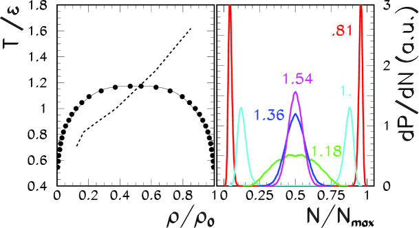
Figure 1: Right part: distributions of the size of the largest cluster in the grancanonical lattice gas model at different temperatures $T/\epsilon$, with a 8x8x8 lattice and at $\mu=3\epsilon$. Left side: lattice gas phas diagram from the distributions on the right side. Dashed line: locus of the maximal $A_{M}$ fluctuation in the canonical ensemble.

In our implementation of the lattice gas model leeyang the $N$ sites of a cubic lattice are characterized by an occupation number $n_{i}$ which is defined as $n_{i}=0(1)$ for a vacancy (particle). Particles occupying nearest neighboring sites interact with a constant coupling $\epsilon$. This model can be transformed into an Ising spin problem with a magnetic field through the mapping $s_{i}=n_{i}-1/2$. The relative particle density $\rho/\rho_{0}$ is defined as the number of occupied sites divided by the total number of sites and is linked to the magnetization of the Ising model by $\rho/\rho_{0}=m+1/2$. In addition to this interaction part a kinetic energy is introduced. Occupied sites are characterized by a momentum vector. Observables expectation values are evaluated in the different ensembles (grancanonical, canonical and microcanonical) sampled through standard Metropolis algorithms commande . The chemical potential in the grancanonical implementation plays the role of the magnetic field $h=\mu-3\epsilon$ in Ising, while the canonical Lattice Gas corresponds to the constant magnetization Ising IMFM case with $m=\rho/\rho_{0}-1/2$.

The phase diagram of the model can be easily evaluated looking at the distribution of the total number of particles $A_{t}=\sum_{i=1}^{N}n_{i}$ in the grancanonical ensemble with a chemical potential $\mu=\mu_{c}=3\epsilon$ which corresponds to the Ising critical field $h=0$. The $A_{t}$ distributions, $P_{\beta\mu}(A_{t})$, are displayed at different temperatures in the right part of figure 1. The presence of two different ensembles of states (bimodality) is clearly seen for all temperatures $T<T_{c}\approx 1.22\epsilon$. At the critical chemical potential $\mu_{c}$ presented in the figure, the probabilities of occurrence of the two solutions are exactly identical; if $\mu<\mu_{c}$ ($\mu>\mu_{c}$) the high (low) density peak dominates. For a fixed temperature $\beta^{-1}$, the most probable $A_{t}$ as a function of $\mu$ is discontinuous at the transition point $\mu_{c}$.

At the thermodynamic limit, the discontinuity in the most probable $A_{t}$ as a function of $\mu$ give rise to a discontinuity in the associated $\langle A_{t}\rangle(\mu)$ equation of state; this implies that the two peaks represent two coexisting phaseszeroes ; topology and that the number of particles ( or equivalently the density) is the order parameter of a phase transition which is first order up to the critical point $T=T_{c}$. The phase diagram can be constructed by reporting the forbidden region for the most probable density i.e. the locus of the discontinuity in the most probable. This corresponds to the two peaks in the bimodal particle number distribution observed at $\mu_{c}$. The phase diagram is displayed in the left part of figure 1. These findings obtained in a 8x8x8 lattice correspond to the phenomenology of the liquid gas phase transition that the model is known to display at the thermodynamic limit. If we increase the lattice size the location of the coexistence border will be modified, even if finite size corrections are especially small in this modelcommande . However it is clear from figure 1 that (except at the critical point which is a second order point, where the two peaks merge to form a single distribution) the first order character of the transition is indisputable even for a linear dimension as small as $L=8$.

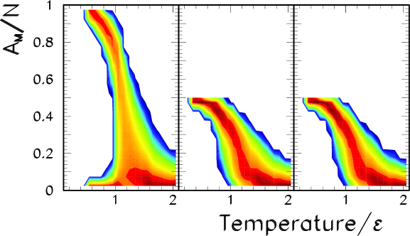
Figure 2: $A_{M}$ distributions as a function of temperature for a 8x8x8 lattice in the grancanonical (left), canonical (middle), and microcanonical (right) ensemble. In all cases the density is $\rho/\rho_{0}=1/2$.

Figure 2 shows the size of the largest cluster $A_{M}$ as a function of the temperature for the grancanonical, canonical and microcanonical ensembles. The obvious correlation between $A_{M}$ and $A_{t}$ implies that for $T<T_{c}$ the $A_{M}$ distribution is also double humped in the grancanonical ensemble as explicitly shown in ref.imfm . This means that $A_{M}$ can also be taken as an order parameter of the liquid gas phase transition, and looking at its distribution this transition can be recognized as first order even for a system constituted of $\langle A_{t}\rangle=256$ particles.

III Conservation laws and thermodynamics

If the constraint of mass conservation is implemented (canonical lattice gas, or equivalently Ising model with fixed magnetization) the distributions of $A_{M}$ drastically changeimfm . In the grancanonical ensemble at $\langle\rho/\rho_{0}\rangle=1/2$, the explored microstates essentially populate the coexistence border, while the coexistence region is accessed with a negligible probability (see figure 1); these highly improbable of the grancanonical distributions are conversely the only microstates which are allowed by the canonical constraint at the value $\rho/\rho_{0}=1/2$ below the transition temperature the grand canonical and canonical partitions differ drastically. Because of the mass conservation constraint, the bimodality of the $A_{t}$ distribution is obviously lost in the canonical ensemble; as a consequence of the correlation between $A_{t}$ and $A_{M}$, the $A_{M}$ distribution also shows a unique peak (figure 2). If we additionally implement a total energy conservation constraint (microcanonical ensemble, right part of figure 2) the distributions get still narrower, but the qualitative behavior is the same than in the canonical ensemble. The normal behavior of the $A_{M}$ distribution at subcritical temperatures may intuitively suggest a pure phase or a continuous transition for the canonical model. This intuition is however false; the characteristics and order of the transition do not depend on the statistical ensemble, and the phase diagram of figure 1 is still pertinent to the canonical ensembleimfm . Indeed the relation between the two ensembles can be written as

$$\log P_{\beta\mu}(A_{t})=\log Z_{\beta}(A_{t})+\beta\mu A_{t}-\log Z_{\beta\mu}$$ (1)

where $Z_{\beta\mu}$, $Z_{\beta}(A_{t})$ are the partition sums in the two ensembles. Eq.(1) shows that in the whole region where the grancanonical distribution $P_{\beta\mu}(A_{t})$ is convex, the canonical equation of state

$$\mu_{can}=-\frac{1}{\beta}\frac{\partial\log Z_{\beta}}{\partial A_{t}}$$ (2)

presents a back bending, which is an unambiguous signal of a first order phase transitiongross . At each temperature the maxima of $P_{\beta\mu}$ correspond to the two ending points of the tangent construction for eq.(2), i.e. to the borders of the coexistence region in the canonical ensemble.

The qualitative behavior of $A_{M}(T)$ in the canonical ensemble does not change with the density of the system. In particular, the $A_{M}$ fluctuation passes systematically through a maximum. The locus of these maxima is displayed on the phase diagram in figure 1. We can see that the maximum fluctuation approximately corresponds to the transition temperature only at the critical point. At subcritical densities this maximum lies inside the coexistence region of the first order phase transition. The results of figure 2 show that the double hump criterium for a first order phase transition does not hold if a constraint is put on a variable closely correlated to the order parameter under study.

IV Conservation laws and Delta scaling

We can ask the question whether a detailed study of the scaling properties of the $A_{M}$ distribution may give extra information on the transition and discriminate first and second order. Following the arguments of ref.botet we consider the distribution

$$\Phi(z)=\Phi\left(\frac{A_{M}-A_{M}^{*}}{\langle A_{M}\rangle^{\Delta}}\right)=\langle A_{M}\rangle^{\Delta}P(A_{M})$$ (3)

where $A_{M}^{*}$ is the most probable value of $A_{M}$ and $0<\Delta\leq 1$ is a real number. At a continuous phase transition point the distribution of the order parameter is expected to fulfil the first scaling law, i.e. the distribution $\Phi$ should be scale invariant with $\Delta=1$. The scale invariance of $\Phi$ for a given value of $\Delta$ is generically refered to as $\Delta$ scaling, and the transition observed experimentallyfrankland from a $\Delta\approx 1/2$ to a $\Delta\approx 1$ scaling by varying the centrality of the collision and therefore the energy deposited in the system, has been taken as a signal of a continuous phase transition.

A practical difficulty in testing $\Delta$ scaling is that for a given distribution the value of $\Delta$ that corresponds to scale invariance, if any, cannot be known a-priori. This difficulty can be circumvented using the fact that the scaling (3) imposed $<A_{M}>^{\Delta}\propto\sigma$. Then it is immediate to verify that eq.(3) can be equivalently written as the ensemble of the two conditions

$$\Psi\left(\frac{A_{M}-\widetilde{A}_{M}}{\sigma_{A_{M}}}\right) = \sigma_{A_{M}}P(A_{M})$$ (4)

$$\sigma^{2}_{A_{M}} = K\langle A_{M}\rangle^{2\Delta}$$ (5)

where $\Psi$ is a scale invariant distribution and $K$ is a constant. Since in presence of a scaling, the difference between the most probable $A_{M}^{*}$ and the average $<A_{M}>$ scales like $\sigma$, $\widetilde{A}_{M}$ can either be one or the other. In the later case the occurence of $\Delta$ scaling study coresponds to the invariance of the centered and reduced distribution. If this distribution does not show scale invariance, we can exclude the existence of any $\Delta$ scaling law. If the function $\Psi$ is scale invariant, this corresponds to a $\Delta$ scaling if and only if the log-log correlation between the average and the variance is linear; in this case the slope of the correlation gives the value of $\Delta$. The practical advantage of testing eqs.(4,5) instead of eq.(3) is that we can check scale invariance without any a-priori knowledge of $\Delta$.

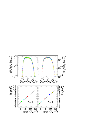
Figure 3: Delta scaling analysis for the canonical lattice gas model at the critical point $\rho=\rho_{0}/2,T=T_{c}$ (left side) and inside coexistence $\rho=\rho_{0}/4$ at the point of maximal $A_{M}$ fluctuation (right side). Upper part: centered and reduced $A_{M}$ distributions. Lower part: correlation between the first two moments and linear interpolation according to eq.(5). The linear size of the lattice is varied as $L=5,6,8,12,16$.

The standard way of testing scale invariance is to consider a specific point of the phase diagram and consider the centered and reduced $A_{M}$ distributions obtained by varying the size of the lattice and, as a consequence, the total number of particles. For the canonical case at the thermodynamical critical point, this analysis is shown on the left side of figure 3. Both eq.(4) and eq.(5) are well verified, in agreement with the expectation of a first scaling law at a continuous transition pointbotet . A comparable quality scaling is however observed also at subcritical densities at the temperature corresponding to the maximum $A_{M}$ fluctuations (right side of figure 3). This finding is in agreement with ref.carmona . Together with the analysis of the phase diagram this means that such a scaling also approximately applies in the coexistence region of a first order phase transition, if the order parameter is not free to fluctuate but is constrained by a conservation law.

V Delta scaling as a function of the system excitation

In the experimental application to nuclear multifragmentationfrankland the system size cannot be varied as freely as in the lattice gas, since the maximum size for a nuclear system is of the order of 400 particles. To explore different values of $\langle A_{M}\rangle$, the same system has been studied at different bombarding energiesfrankland and/or different impact parametersfrankland_new . In a similar way, we have kept the total number of particles constant and we have varied the temperature. To fix the ideas, we have chosen the simplest thermodynamical path from coexistence to the fluid phase passing through the critical point, $\rho(T)=cte=\rho_{0}/2$. The resulting $\Psi$ functions are displayed in figure 4. No scaling is observed: the function $\Psi$ continuously evolves from a distribution with a tail extending towards the low mass side compared to the average at low temperature while the opposite is true at high temperature.

If we look at the behavior of the variance as a function of the first moment, the log-log correlation is nowhere linear showing that the large fragment fluctuation does not evolve like a power of the average fragment size. The bell shaped behavior of this curve is due to the mass conservation constraint, that forces the fluctuation to vanish both at low and at high $\langle A_{M}\rangle$ values. The observed maximum is in fact the maximum fluctuation point shown in figure 1 which, at the critical density, occurs close to the critical point and, for sub-critical densities, is located inside the coexistence region.

To qualitatively compare with experimental $\Delta$-scaling analysis, we have to remember that the studied experimental distributions only cover the multifragmentation regime and do not explore the decreasing part of the $\sigma_{A_{M}}(\langle A_{M}\rangle)$ correlation which would correspond in the nuclear case to evaporation from a compound. Focusing now on the fragmentation region, we show in figure 4 the best power law interpolations of the average and variance correlation to be compared with the published experimental analysis presenting a $\Delta=1$ to a $\Delta=1/2$ regime. In this interpretation, the crossing point between the two power-law fits is interpreted as a ”transition” point. By construction it appears to be at a higher temperature then the maximum fluctuation which at this critical density comes out to be close to the critical temperature.

To better study the possible occurrence of a power law scaling of the large fragment fluctuation we can study the double logarithmic derivative

$$\Delta^{\prime} = \frac{d\sigma_{A_{M}}}{d\langle A_{M}\rangle}$$ (6)

In presence of a $\Delta$-scaling this quantity should be constant. Figure 4 shows that $\Delta^{\prime}$ is a smoothly decreasing function passing through the values $1$ and $1/2$ before going through $0$ at the maximum fluctuation point and then becoming negative as a consequence of the mass conservation law. No plateaus of $\Delta^{\prime}$ are observed confirming the absence of scaling.

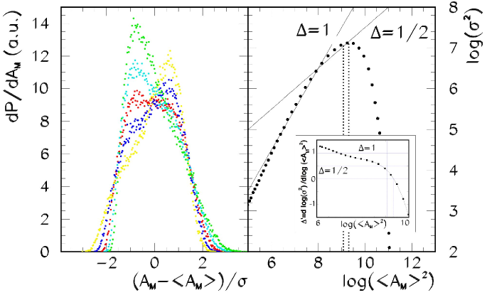
Figure 4: Delta scaling analysis for the canonical lattice gas model at constant density $\rho=\rho_{0}/2$ varying the system temperature. Left part: centered and reduced $A_{M}$ distributions for temperatures varying from $T=1.1\epsilon$ to $T=1.25\epsilon$. Right part: correlation between the first two moments and linear interpolations according to eq.(5). Temperatures range from $T=.3\epsilon$ to $T=2.3\epsilon$. The vertical lines indicate the temperature of maximum $A_{M}$ fluctuations and the critical temperature. The double logarithmic derivative $\Delta^{\prime}$ is shown in the inserted figure.

This violation of scaling occurs in spite of the fact that a continuous phase transition point (the thermodynamic critical point) is explored in the simulations. At this point the distributions indeed follow the first scaling law (left part of figure 3) but this information is lost if the different distributions are generated by varying the temperature. This is not only true for the transition point, but also for the supercritical regime. Indeed this regime has been shown to exhibit the second scaling law $\Delta=1/2$ in the Potts modelbotet (or something close to it $\Delta\approx 0.6$ for the IMFMcarmona ), while in the representation of figure 4 scaling can everywhere be excluded.

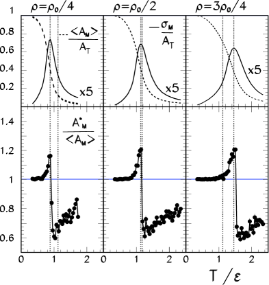
Figure 5: First moments of the $A_{M}/A_{T}$ distribution as a function of temperature for a 8x8x8 lattice in the canonical ensemble at $\rho/\rho_{0}=1/4$ (left),$\rho/\rho_{0}=1/2$ (medium), and $\rho/\rho_{0}=3/4$ (right). Upper part: mean value (full line) and variance (dashed line). Lower part: most probable value of the $A_{M}$ distribution normalized to the mean. The vertical lines indicate the temperature of maximal $A_{M}$ fluctuations and the transition temperature for each density.

The conclusion is that scale invariance can only be tested by varying the total system size. However other information on the phase transition can be accessed through the study of the $A_{M}$ distribution with a fixed total number of particles, as we now show.

VI Signals of phase transition and of its order

The first two moments of the distribution in the canonical ensemble and the corresponding most probable value $A_{M}^{*}$ are displayed in figure 5 for three different densities. Let us look at the $\rho<\rho_{c}$ case first. If the first and second moment show smooth behaviors dominated by the conservation law constraint, the transition is still apparent in the behavior of $A_{M}^{*}$ which rapidly changes at a temperature close to the transition point. This sudden decrease is due to a change of sign in the asymmetry of the distribution. As such, the qualitative behavior of $A_{M}^{*}(T)$ is independent of the density. A great number of continuous transition signals has been observed in different mass conserving models at densities that do not correspond to a continuous phase transitioncarmona ; dasgupta ; bugaev ; commande ; fisher ; raduta . The same happens for the most probable value of $A_{M}$. This variable shows for all densities a sudden drop at a temperature $T_{t}(\rho)$ which corresponds to the maximum of the $A_{M}$ fluctuations. As we have already stressed, these temperatures approximately coincide with the transition temperature only at the critical density (see figure 1). The behavior at supercritical densities reflects a geometric phase transition which has no thermodynamic counterpart, while if fragmentation takes place at low density the $A_{M}$ drop can be taken as a signal of phase coexistence.

In order to discriminate between the different density regimes and recognize the order of the phase transition, we have to quantify the $A_{M}$ fluctuation peak. In the grancanonical ensemble, the $A_{t}$ fluctuation is directly linked to the susceptibility via

$$\chi=\frac{\partial\langle A_{t}\rangle}{\partial\mu}=\beta(\sigma_{A_{t}}^{\mu})^{2}$$ (7)

To work out a similar expression for the canonical ensemble, let us assume that $A_{M}$ and the other fragments are statistically independent, i.e. the total density of states is factorized

$$W_{t}(A_{M},A_{m},E_{M},E_{m})=W_{M}(A_{M},E_{M})\cdot W_{m}(A_{m},E_{m})$$ (8)

where we have defined the total number of particles not belonging to the largest fragment as $A_{m}=A_{t}-A_{M}$, and the corresponding energy $E_{m}=E_{t}-E_{M}$. This hypothesis is reasonably well verified in the Lattice Gas model, since the correlation coefficient between $A_{M}$ and $A_{m}$ in the grancanonical ensemble comes out to be close to zero except in the very dense regime $\rho/\rho_{0}\approx 1$. The factorization of the state densities implies a convolution of the corresponding canonical partition sums

$$Z_{\beta}(A_{t}) = \int dE_{t}e^{-\beta E_{t}}\int_{0}^{E_{t}}dE_{m}\int_{0}^{A_{t}}dA_{m}\cdot W_{m}(E_{m},A_{m})W_{M}(E_{t}-E_{m},A_{t}-A_{m})$$ (9)

$$= \int_{0}^{A_{t}}dA_{m}Z_{\beta}^{M}(A_{M})Z_{\beta}^{m}(A_{t}-A_{M})$$

where $Z_{\beta}^{i},i=m,M$ describe the contribution of the largest fragment and of all the others respectively.

The distribution of the largest fragment reads

$$P_{\beta A_{t}}(A_{M})=Z_{\beta}^{-1}(A_{t})Z^{M}_{\beta}(A_{M})Z^{m}_{\beta}(A_{t}-A_{M})$$ (10)

A Gaussian approximation of this distribution leads tonpa

$$\beta\sigma^{2}_{A_{M}}=\left(\frac{1}{\chi_{m}(A_{t}-A_{M}^{*})}-\frac{1}{\chi_{M}(A_{M}^{*})}\right)^{-1}$$ (11)

where $\sigma^{2}_{A_{M}}$ is the fluctuation of the $A_{M}$ distribution and the partial susceptibilities are defined as $\chi^{-1}_{i}=\frac{\partial\mu_{i}}{\partial A_{i}}(A^{*}_{i})$.

The above derivation is valid for a system whose state density depends on the two extensive variables, number of particles $A$ and energy $E$. In the case of the fragmentation transition a third extensive variable, the volume $V$, has also to be considered. We show in the appendix that in this more general case eq. (11) can still be derived, but a dilute limit $V_{t}=V_{m}+V_{M}\approx V_{m}$ has to be considered.

According to the general definition of phase transitions in finite systemsgross ; houches , the generalized susceptibility associated to an order parameter is negative in a first order phase transition in the statistical ensemble where the order parameter is subject to a conservation law. We therefore expect a negative $\chi_{M}$ at subcritical densities. Imposing $\chi_{M}<0$ in eq.(11) leads to

$$\sigma^{2}_{A_{M}}>\beta^{-1}\chi_{m}(A_{t}-A_{M}^{*})$$ (12)

Comparing to eq.(7) this finally gives

$$\sigma^{2}_{A_{M}}=\sigma^{2}_{A_{m}}>(\sigma^{\mu}_{A_{m}})^{2}$$ (13)

Equation (13) associates the first order phase transition in the canonical ensemble to ”abnormal” $A_{M}$ fluctuations, in the same way as abnormal partial energy fluctuations sign a first order phase transition in the microcanonical ensemblenpa .

Figure 6: Ratio between the grancanonical and canonical fluctuation of the number of particles $A_{m}$ not belonging to the largest cluster, as a function of the temperature for a 8x8x8 lattice at $\rho/\rho_{0}=1/4$ (left),$\rho/\rho_{0}=1/2$ (medium), and $\rho/\rho_{0}=3/4$ (right). Dashed lines: average canonical $A_{M}$ values normalized to the total number of particles. Vertical lines in the two left panels: limit of the region of negative susceptibility from the canonical $\mu(A)$ equation of state eq.(2) commande .

The canonical and grancanonical fluctuations are compared in figure 6 for three different densities. Independent of the system density our approximation eq.(13) turns out to be incorrect at very low temperatures, when the average size of the largest cluster (dashed lines) exceeds about 80% of the available mass. In this case the hypothesis of statistical independence between $A_{m}$ and $A_{M}$ cannot be justified and the canonical mass conservation costraint trivially reduces the canonical fluctuation. However as soon as the average $A_{M}$ value drops, we can see that the region of negative susceptibility can be well reconstructed through eq.(13), and in particular its border (vertical lines) is very precisely determined by the equality condition between the two fluctuations. At supercritical densities the dilute gas approximation we have employed breaks down independent of the temperature and the susceptibility cannot quantitatively be estimated from the fluctuation signal, however in this regime the relative fluctuation observable does not present any peak while only inside the spinodal region of the first order phase transition the canonical fluctuation exceeds the grancanonical one. It is clear that this observable allows a unambiguous discrimination between the supercritical regime and phase coexistence.

VII Conclusions

To conclude, in this paper we have discussed the role of the largest fragment in the framework of the lattice gas model. We have shown that this variable can be taken as an order parameter of the fragmentation phase transition if this latter belongs to the liquid gas universality class. It has been already observed carmona ; pliemling that the phase transition can be tracked from the sudden drop of $A_{M}$ close to the transition temperature. This drop is well fitted by a power law with a $\beta$ exponent close to the expected value for the liquid gas universality classpliemling but finite size effects blur the behavior considerably for system sizes comparable to accessible nuclear sizes. However, when no constraints are affecting the fluctuations of the order parameter such as in the grand canonical ensemble, we have shown that the transition is very well defined if instead of the average we look at the most probable value of $A_{M}$. Indeed crossing a first order phase transition point this variable is discontinuous independent of the system size. The important result is that if we look at this variable finite size effects do not constitute a major problem to identify a phase transition nor to recognize its order.

On the other hand important ambiguities arise from the non equivalence of statistical ensembles inside a phase transition. Indeed the distribution of the order parameter is strongly deformed by the presence of conservation laws in the system under study. If we look at $A_{M}$ as an order parameter, the double hump criterium for a first order phase transition does not apply any more in the canonical or microcanonical ensemble because of the strong correlation between the conserved total number of particles and the order parameter. The mass conservation constraint induces a maximum in the fluctuation of $A_{M}$ which is not necessarily correlated with the properties of the phase diagram. We observe maxima both at the critical density close to the critical point and at sub-critical densities inside the coexistence zone. Moreover, the presence of this maximum can simulate a transition from a $\Delta=1$ to a $\Delta=1/2$ scaling law in a region above the maximum fluctuation. It is clear that other observables have to be employed if we want to conclude about the order and nature of the phase transition. One such observable is the numerical value of the fluctuation of $A_{M}$, which is by construction identical to the fluctuation of the number of particles that do not belong to the largest cluster $A_{m}$: if and only if the system crosses the phase coexistence region of a first order phase transition, this fluctuation overcomes the corresponding value in the grancanonical ensemble.

VIII Appendix: derivation of eq.(10)

The density of states is a function of all the relevant extensive variables of the system. For the lattice gas model this means $W=W(E,A,V)$. If the largest fragment $A_{M}$ is statistically independent from the other clusters then

$$W_{t}(A_{M},E_{M},V_{M},A_{m},E_{m},V_{m})=W_{M}(A_{M},E_{M},V_{M})\cdot W_{m}(A_{m},E_{m},V_{m})$$ (14)

where we have defined the total number of particles not belonging to the largest fragment as $A_{m}=A_{t}-A_{M}$, and the corresponding energy and volume $E_{m}=E_{t}-E_{M}$,$V_{m}=V_{t}-V_{M}$. Let us first consider the case of an external temperature $T=\beta^{-1}$ and pressure $p=\beta\lambda$. Using the standard definition of the canonical isobar partition sum

$$Z_{\beta\lambda}(A)=\int dEe^{-\beta E}\int dVe^{-pV}W(E,A,V)$$

the total partition sum can be written as

$$Z_{\beta\lambda}(A_{t}) = \int dE_{t}e^{-\beta E_{t}}\int dV_{t}e^{-pV_{t}}\int_{0}^{E_{t}}dE_{m}\int_{0}^{V_{t}}dV_{m}\int_{0}^{A_{t}}dA_{m}\cdot$$

$$W_{m}(E_{m},A_{m},V_{m})W_{M}(E_{t}-E_{m},A_{t}-A_{m},V_{t}-V_{m})$$

or equivalently

$$Z_{\beta}(A_{t})=\int_{0}^{A_{t}}dA_{m}Z_{\beta}^{M}(A_{M})Z_{\beta}^{m}(A_{t}-A_{M})$$ (15)

where $Z_{\beta}^{i},i=m,M$ describe the contribution of the largest fragment and of all the others respectively. In the isochore case $V_{m}+V_{M}$=cte, the convolution of the partition sum is less straightforward because of the presence of the volume integral

$$Z_{\beta}(A_{t},V_{t})=\int_{0}^{A_{t}}dA_{m}\int_{0}^{V_{t}}dV_{m}Z_{\beta}^{M}(A_{M},V_{M})Z_{\beta}^{m}(A_{t}-A_{M},V_{t}-V_{M})$$ (16)

Let us introduce the partial pressures $p_{i}=\beta^{-1}\frac{\partial lnZ_{\beta}^{i}}{\partial V_{i}}(A^{*}_{i},V^{*}_{i})$ and chemical potentials $\mu_{i}=\beta^{-1}\frac{\partial lnZ_{\beta}^{i}}{\partial A_{i}}(A^{*}_{i},V^{*}_{i})$ at the most probable volume and mass partition $A^{*}_{M},V^{*}_{M}$. Equilibrium between the two components implies $\mu_{m}=\mu_{M}$, $p_{m}=p_{M}$. A saddle point approximation then gives

$$Z_{\beta}^{M}Z_{\beta}^{m}\approx exp \left(-\beta\left[A^{*}_{M}f_{M}+A^{*}_{m}f_{m}\right]\right)\cdot$$

$$exp \left(-\beta\left[\frac{1}{2}\left(A_{m}-A^{*}_{m}\right)^{2}\left(\chi_{M}^{-1}+\chi_{m}^{-1}\right)+\frac{1}{2}\left(V_{m}-V^{*}_{m}\right)^{2}\left(\kappa_{M}^{-1}+\kappa_{m}^{-1}\right)\right]\right)\cdot$$

$$exp \left(-\beta\left[\frac{1}{2}\left(A_{m}-A^{*}_{m}\right)\left(V_{m}-V^{*}_{m}\right)\left(\frac{\partial p_{M}}{\partial A_{M}}+\frac{\partial p_{m}}{\partial A_{m}}\right)\right]\right)$$

where $f_{i}=-TlnZ_{\beta}^{i}(A^{*}_{i})/A^{*}_{i},i=m,M$ are the most probable free energies per particle, the partial susceptibilities and compressibilities are defined as $\chi^{-1}_{i}=\frac{\partial\mu_{i}}{\partial A_{i}}(A^{*}_{i},V^{*}_{i})$, $\kappa^{-1}_{i}=\frac{\partial p_{i}}{\partial V_{i}}(A^{*}_{i},V^{*}_{i})$, and the conservation constraints make the linear terms vanish. In the dilute limit $V_{t}=V_{m}+V_{M}\approx V_{m}$ the density variation of the ”gas” component $m$ is due to its number variation $d\rho_{m}=dA_{m}/V_{t}$ and the volume variation can be neglected respect to the number variation $V_{m}-V^{*}_{m}\ll A_{m}-A^{*}_{m}$ giving

$$Z_{\beta}(A_{t},V_{t})\approx\int_{0}^{A_{t}}dA_{m}Z_{\beta}^{M}(A_{M},V^{*}_{m})Z_{\beta}^{(m)}(A_{t}-A_{M},V_{t}-V^{*}_{m})$$ (17)

Both in the isobar (15) and in the isochore (17) case, the distribution of the largest fragment reads

$$P_{\beta A_{t}}(A_{M})=Z_{\beta}^{-1}Z^{M}_{\beta}(A_{M})Z^{m}_{\beta}(A_{t}-A_{M})$$ (18)

Implementing the saddle point approximation we can identify

$$\beta\sigma^{2}_{A_{M}}=\left(\frac{1}{\chi_{m}(A_{t}-A_{M}^{*})}-\frac{1}{\chi_{M}(A_{M}^{*})}\right)^{-1}$$ (19)

where $\sigma^{2}_{A_{M}}$ is the fluctuation of the $A_{M}$ distribution.

References

- (1) X. Campi, J.Desbois, E.Lipparini, Phys. Lett. 138B (1984) 353.
- (2) K. Binder, D. P. Landau, Phys. Rev. B 30 (1984) 1477.
- (3) R. Botet, M. Ploszajczak, Phys. Rev. E62 (2000) 1825.
- (4) B. Tamain et al., Nucl.Phys.A, in press; M.F.Rivet et al., nucl-ex/0412007.
- (5) R.Botet et al., Phys.Rev.Lett.86(2001)3514.
- (6) C. B. Das, S. Das Gupta and A. Majumder, Phys. Rev. C65 (2002) 34608; C. B. Das et al., Phys. Rev. C66 (2002) 044602.
- (7) K. A. Bugaev et al., Phys. Rev. C62 (2000) 044320 and Phys. Lett. B 498 (2001) 144.
- (8) F.Gulminelli, Ph.Chomaz, Phys.Rev.Lett.82 (1999) 1402; Ph.Chomaz, F.Gulminelli, Int. Journ. Mod. Phys. E8 (1999) 527.
- (9) F. Gulminelli et al., Phys. Rev.C (2002) 51601.
- (10) A. H. Raduta et al., Phys. Rev. C 65, 034606 (2002).
- (11) J. M. Carmona, J. Richert, P. Wagner, Phys. Lett. B531 (2002) 71.
- (12) C.N.Yang, Phys.Rev.85 (1952)809
- (13) A. Coniglio and W. Klein, J. Phys. A13 (1980) 2775; X. Campi, H. Krivine and A. Puente, Physica A 262 (1999) 328.
- (14) F. Gulminelli and Ph. Chomaz, Phys.Rev.E 66 (2002) 046108.
- (15) K. C. Lee, Phys. Rev. 53 E (1996) 6558; Ph. Chomaz, F. Gulminelli, Physica A (2003).
- (16) Ph.Chomaz, F.Gulminelli, V.Duflot, Phys.Rev.E64 (2001) 046114.
- (17) F. Gulminelli et al., Phys. Rev. E 68 (2003) 026120.
- (18) D. H. E. Gross, ”Microcanonical thermodynamics: phase transitions in finite systems”, Lecture notes in Physics vol. 66, World Scientific (2001).
- (19) P.Chomaz and F.Gulminelli, Nucl. Phys. A647 (1999) 153.
- (20) Ph.Chomaz and F.Gulminelli, in ’Dynamics and Thermodynamics of systems with long range interactions’, Lecture Notes in Physics vol.602, Springer (2002).
- (21) J.Frankland et al., nucl-ex/0404024 unpublished.
- (22) M. Pleimling and A. Hueller, J. Stat. Phys. 104 (2001) 971.