Abstract

The theory of QED corrections to hyperfine structure in light hydrogenic atoms and ions has recently advanced to the point that the uncertainty of these corrections is much smaller than 1 part per million (ppm), while the experiments are even more accurate. The difference of the experimental results and the corresponding QED theory is due to nuclear effects, which are primarily the result of the finite nuclear charge and magnetization distributions. This difference varies from tens to hundreds of ppm. We have calculated the dominant nuclear component of the 1s hyperfine interval for deuterium, tritium and singly ionized helium, using a unified approach with modern second-generation potentials. The calculated nuclear corrections are within 3% of the experimental values for deuterium and tritium, but are roughly 20% discrepant for helium. The nuclear corrections for the trinucleon systems can be qualitatively understood by invoking SU(4) symmetry.

1 Introduction

Until very recently hyperfine splittings in light hydrogenic atoms were the most precisely measured atomic transitions. Theoretical predictions based on QED are less accurate, but have improved considerably in recent years. Non-recoil and non-nuclear contributions[1, 2] are known through order $\alpha^{3}E_{\rm F}$, where $E_{\rm F}$ is the Fermi hyperfine energy (viz., the leading-order contribution) and $\alpha$ is the fine-structure constant. Because the hadronic scales for recoil and certain types of nuclear corrections are the same, recoil corrections are treated on the same footing as nuclear corrections[1], and we will call both types “nuclear corrections.” Uncalculated QED terms of order $\alpha^{4}E_{\rm F}$ in light atoms are almost certainly smaller than .1 ppm., while the experimental errors are smaller still. This provides us with the unprecedented opportunity to study nuclear effects in the hyperfine structure (hfs) of light hydrogenic atoms, which range in size from tens to hundreds of ppm. We will restrict ourselves to hydrogenic s-states, because these states maximize nuclear effects.

Table 1: Difference between hyperfine experiments and QED hyperfine calculations for the $n\underline{\rm th}$ s-state of light hydrogenic atoms times $n^{3}$, expressed as parts per million of the Fermi energy. This difference is interpreted as nuclear contributions to the hyperfine splitting[2]. A negative entry indicates that the theoretical prediction without nuclear corrections is too large.

$n^{3}(E_{\rm hfs}^{\rm exp}-E_{\rm hfs}^{\rm QED})/E_{\rm F}\,{\rm(ppm)}$
State	H	2H	3H	3He+
1s	$-$33	138	$-$38	$-$212
2s	$-$33	137	$--$	$-$211

Table 1 is an updated version of the corresponding table in Ref.[2]. Because nuclear effects have a much shorter range than atomic scales, we expect the splittings in the $n\underline{\rm th}$ s-state to be proportional to $|\phi_{n}(0)|^{2}\sim 1/n^{3}$, where $\phi_{n}(r)$ is the non-relativistic wave function of the electron. Forming the fractional differences (in parts per million) between $E^{\rm exp}_{\rm hfs}$ and $E^{\rm QED}_{\rm hfs}$ (times $n^{3}$) leads to the tabulated results. As we stated above, these large differences reflect neither experimental errors nor uncertainties in the QED calculations, but rather the large nuclear contributions to hfs.

In order to perform a tractable calculation it is necessary to restrict the scope, while at the same time incorporating the dominant physics. To accomplish this we borrow a technique from chiral perturbation theory ($\chi$PT, the effective field theory for nuclei based on QCD). This technique, called power counting, is the organizing principle of $\chi$PT and allows one to perform systematic expansions[3] in powers of a small parameter, $(Q/\Lambda)$, where $Q$ is a typical nuclear momentum scale that can be taken to be roughly the pion mass ($m_{\pi}\sim$ 140 MeV), and $\Lambda$ is the large-mass QCD scale ($\sim$ 1 GeV) typical of QCD bound states such as the nucleon, heavy mesons, nucleon resonances, etc. We also note that $1/Q$ specifies a typical correlation length (and a reasonable nearest-neighbor distance) in light nuclei ($\sim$ 1.4 fm)[4]. This expansion in powers of $(Q/\Lambda\sim 0.1-0.15)$ should converge moderately well. In this work we restrict ourselves to leading order in this expansion, and this restriction eliminates nuclear corrections of relativistic order, which are subleading and exceptionally complicated because of the complexity of the nuclear force[5, 6].

In processes that involve virtual excitation of intermediate nuclear states (each with its own energy, $E_{N}$, relative to the ground-state energy, $E_{0}$) the excitation energy $(\omega_{N}=E_{N}-E_{0})$ is of order $Q^{2}/\Lambda$ and typically is a correction to the leading order[4]. Consistency therefore demands that we drop such terms. The nuclear recoil energy scales like $Q^{2}/M$, where $M$ is the nucleon mass, and can also be dropped. These are very considerable simplifications in constructing the nuclear contribution to hfs, which we present in the next section.

2 Nuclear Contributions to Hyperfine Structure

The hyperfine interactions that interest us are simple (effective) couplings of the electron spin to the nuclear (ground-state) spin: $\vec{\sigma}\cdot\vec{S}$, where $\vec{\sigma}$ is the electron (Pauli) spin operator and $\vec{S}$ is the nuclear spin (total angular momentum) operator. Other couplings of the electron spin are possible and either generate no hyperfine splitting, none in s-states, or higher-order (in $\alpha$) contributions.

The lowest-order (Fermi) hyperfine interaction is generated by the interaction of the electron current with the magnetic dipole part (determined by $\vec{\mu}$) of the nuclear current. A simple calculation gives the well-known result[1]

$$E_{\rm F}=\frac{4\pi\alpha\mu_{N}|\phi_{n}(0)|^{2}}{3m_{e}}\frac{\vec{\sigma}\cdot\vec{S}}{S}\,,$$

where $\langle SS|\mu_{\rm z}|SS\rangle\equiv\mu_{N}$ defines the nuclear magnetic moment and $m_{e}$ is the electron mass. The factor of $(\vec{\sigma}\cdot\vec{S})/S$ leads to a hyperfine splitting proportional to $(2\,S+1)/S$. All additional contributions will be measured as a fraction of this energy.

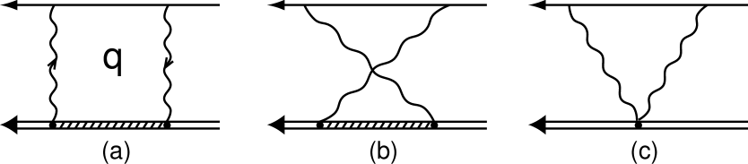
Figure 1: Nuclear Compton amplitude with direct (a), crossed (b), and seagull (c) contributions illustrated. Single lines represent an electron, double lines a nucleus, and shaded double lines depict a nuclear Green’s function containing a sum over nuclear states. The seagull vertex maintains gauge invariance. The four-momentum running through the loop is $q^{\mu}$.

Naively calculating the higher-order (in $\alpha$) corrections using only the nuclear magnetization distribution will fail. The atomic wave function is modified by the nuclear charge distribution in precisely the same region that the magnetization distribution is nonvanishing[7, 8]. It is therefore necessary to incorporate the complete set of second-order (in perturbation theory in $\alpha$) processes shown in Fig (1), which comprise the nuclear Compton amplitude coupled to the electron Compton amplitude. Only the forward-scattering part of this amplitude is required for the ${\cal O}(\alpha)$ corrections to $E_{\rm F}$. The resulting energy shift is then given by

$$\Delta E=i(4\pi\alpha)^{2}|\phi_{n}(0)|^{2}\int\frac{d^{4}q}{(2\pi)^{4}}\frac{t_{\mu\nu}(q)\,T^{\mu\nu}(q,-q)}{(q^{2}+i\epsilon)^{2}(q^{2}-2m_{e}q_{0}+i\epsilon)}\,,$$

where $t^{\mu\nu}$ is the electron Compton amplitude and $T^{\mu\nu}$ is the nuclear Compton amplitude, which is required to be gauge invariant. The lepton tensor can be decomposed into an irreducible spinor basis, and we can ignore odd matrices and spin-independent components.

We also ignore (for now) terms that couple two currents together. It is easy to show that since the nuclear current scales as $1/\Lambda$ (the conventional components of the current have explicit factors of $1/M$), two of them should scale as $1/\Lambda^{2}$ and generate higher-order (in $1/\Lambda$) terms. This leaves a single dominant term representing a charge-current correlation

$$\Delta E=(4\pi\alpha)^{2}|\phi_{n}(0)|^{2}\int\frac{d^{4}q}{(2\pi)^{4}}\frac{(\vec{\sigma}\times\vec{\,q})^{m}[T^{m0}(q,-q)-T^{0m}(q,-q)]}{(q^{2}+i\epsilon)^{2}(q^{2}-2m_{e}q_{0}+i\epsilon)}\,.$$

The nuclear seagull terms $B^{0m}(q,-q)$ and $B^{m0}(q,-q)$ that are contained as part of $T^{\mu\nu}$ in Fig. (1c) are of relativistic order[5] $(\sim 1/\Lambda^{2})$ and can be dropped. Although the seagull terms $B^{mn}(\vec{\,q},-\vec{\,q})$ are of non-relativistic order, they do not contribute to hfs because of crossing symmetry. The explicit form for the remaining term in $T^{m0}$ (suppressing the nuclear ground-state expectation value), which involves a complete sum over intermediate states, $N$, is given by

$$T^{m0}(q,-q)=\sum_{N}\frac{J^{m}(-\vec{\,q})\,|N\rangle\langle N|\,\rho(\vec{\,q})}{q_{0}-\omega_{N}+i\epsilon}+{\rm crossed\;term}\,,$$

where $\vec{J}(\vec{\,q})$ and $\rho(\vec{\,q})$ are the Fourier transforms of the nuclear current and charge operators. The crossed term has the operator order reversed and $q_{0}\rightarrow-q_{0}$.

The limits $\omega_{N}\rightarrow 0$ and $m_{e}\rightarrow 0$ (both scales are small compared to the nuclear-size scale, $1/Q$) greatly simplify the calculation, and this leads to

$$\Delta E=i\,(4\pi\alpha)^{2}|\phi_{n}(0)|^{2}\int\frac{d^{3}q}{(2\pi)^{3}}\frac{(\vec{\sigma}\times\vec{\,q})^{m}\{J^{m}(-\vec{\,q}),\rho(\vec{\,q})\}}{\vec{\,q}^{6}}\,,$$

which is infrared divergent. Using

$$J^{m}(-\vec{\,q})=\int d^{3}y\,J^{m}(\vec{y})\exp{(-i\vec{\,q}\cdot\vec{y})}\,,$$

and

$$\rho(\vec{\,q})=\int d^{3}x\,\rho(\vec{x})\exp{(i\vec{\,q}\cdot\vec{x})}\,,$$

together with $\vec{z}\equiv\vec{x}-\vec{y}$, and a lower-limit (infrared) $q-$cutoff, $\epsilon$, we find

$$\Delta E=-8\alpha^{2}|\phi_{n}(0)|^{2}\int d^{3}x\int d^{3}y\,\{\rho(\vec{x}),\vec{\sigma}\cdot\vec{J}(\vec{y})\}\times\vec{\nabla}_{z}(\frac{1}{3\epsilon^{3}}-\frac{z^{2}}{6\epsilon}+\frac{\pi z^{3}}{48})\,,$$

where there is an implied (nuclear and atomic) expectation value. The constant term does not contribute because of the derivative. The second term is only logarithmically divergent when Siegert’s theorem is applied[9], can be shown to vanish in several limits (including the zero-range limit), and is consequently negligibly small[10]. The last term is the one we are seeking and was originally developed by Low[11] in a limiting case for the deuteron, after the basic concept was sketched by Bohr[12]:

$$\Delta E^{\rm Low}_{\rm hfs}=\frac{\pi\alpha^{2}|\phi_{n}(0)|^{2}}{2}\int d^{3}x\int d^{3}y\,|\vec{x}-\vec{y}|\,\{\rho(\vec{x}),\vec{\sigma}\cdot(\vec{x}-\vec{y})\times\vec{J}(\vec{y})\}\,+\cdots\,.$$

A more convenient representation can be obtained by dividing both sides of this equation by the expression for the Fermi hyperfine energy given by Eqn. (1). Since the Wigner-Eckart theorem guarantees that Eqn. (8) must be proportional to $\vec{\sigma}\cdot\vec{S}/S$ (which cancels in the ratio), we arrive at a simple expression for the leading-order nuclear contribution to the hfs, which is one of our primary results.

$$\Delta E^{\rm Low}_{\rm hfs}/E_{\rm F}=-2\,m_{e}\,\alpha\,\delta_{\rm Low}\,,$$

where

$$\delta_{\rm Low}=-\frac{3}{16\mu_{N}}\int d^{3}x\int d^{3}y\,|\vec{x}-\vec{y}|\,\{\rho(\vec{x}),((\vec{x}-\vec{y})\times\vec{J}(\vec{y}))_{\rm z}\}\,,$$

and a nuclear expectation value is required of the z (or “3”) component of this vector in the nuclear state with maximum azimuthal spin (i.e. $S_{\rm z}=S$). The intrinsic size of the nuclear corrections is given by ($-2\,m_{e}\,\alpha R$) = $-$38 ppm $[R/$fm], where $[R/$fm] is the value of the Low moment in Eqn. (10) in units of fm.

3 Nuclear Matrix Elements

In order to evaluate Eqn. (10) it is necessary to assume a form for the nuclear charge and current operators. We have agreed to ignore terms of relativistic order, and this eliminates all but the usual impulse-approximation (i.e., one-body) terms for the charge operator, which contains finite-size distributions for the protons and neutrons. Although the latter contributions are small, they have never been included in previous calculations and we will gauge their importance by including them in our calculation. The nuclear current operator can be written in terms of the dominant spin-magnetization current, the convection current (motional current of charged particles) and meson-exchange currents (MEC). Isoscalar MEC are of relativistic order[5] and we ignore them. Isovector MEC are larger, but don’t contribute to the deuteron because it is an isoscalar nucleus. Isovector MEC will contribute to the trinucleon systems, where the effect of this current on the isovector magnetic moment is about the same size (15%) as our expansion parameter[13]. Because parts of these currents (in particular the isobar part) are difficult to treat quantitatively and because of their relative smallness, we will ignore MEC in calculating the Low moments in this initial effort to understand hfs in the trinucleon systems.

Each of the charge and current operators that we use are therefore given by sums of one-body operators, and their resulting product in the Low-moment expression in Eqn. (10) can be written as a sum of one-body terms plus a sum of two-body terms. Using a transparent notation for this decomposition ($\delta_{\rm Low}=\delta^{(1)}_{\rm spin}+\delta^{(2)}_{\rm Low}$ and $\delta_{\rm Low}^{(2)}=\delta_{\rm Low}^{\rm mag}+\delta_{\rm Low}^{\rm conv}$) we find that the one-body term is given for all nuclei by the spin-magnetization current in the form

$$\delta_{\rm spin}^{(1)}=\langle r\rangle^{pp}_{(2)}\frac{\mu_{p}}{\mu_{N}}\sum_{i=1}^{A}\left(\frac{1+\tau^{3}_{i}}{2}\right)\sigma_{i}^{\rm z}+\langle r\rangle^{nn}_{(2)}\frac{\mu_{n}}{\mu_{N}}\sum_{i=1}^{A}\left(\frac{1-\tau^{3}_{i}}{2}\right)\sigma_{i}^{\rm z}\,,$$

where

$$\langle r\rangle^{pp}_{(2)}=\int d^{3}x\int d^{3}y\,\rho^{p}_{ch}(x)\,\rho^{p}_{M}(y)|\vec{x}-\vec{y}|=1.086(12){\,\rm fm}\,$$

and

$$\langle r\rangle^{nn}_{(2)}=\int d^{3}x\int d^{3}y\,\rho^{n}_{ch}(x)\,\rho^{n}_{M}(y)|\vec{x}-\vec{y}|\,$$

determine the proton and neutron parts, respectively, of the one-body current. The quantities $\vec{\tau}_{i}$ and $\vec{\sigma}_{i}$ are the (Pauli) isospin and spin operators for the ith nucleon, $\rho^{p}_{ch}$, $\rho^{p}_{M}$, and $\rho^{n}_{M}$ are the proton charge and magnetic densities and the neutron magnetic density (normalized to 1), while $\rho^{n}_{ch}$ is the neutron charge density (normalized to 0). Note that the quantities $\langle r\rangle^{pp}_{(2)}$ and $\langle r\rangle^{nn}_{(2)}$ are the proton and neutron Zemach moments[8, 14], and we have listed in Eqn. (12a) the value of the proton Zemach moment recently determined directly from the electron-scattering data for the proton[15] (the neutron has not yet been evaluated). In numerical work described below we will use simple forms for the neutron and proton form factors: a dipole form for the proton charge and magnetic form factors and the neutron magnetic form factor $(F_{D}(q^{2})=\frac{1}{(1+q^{2}/\beta^{2})^{2}})$ and a modified Galster[16] form for the neutron charge form factor $(F_{G}=\frac{\lambda q^{2}}{(1+q^{2}/\beta^{2})^{3}}$, where $\lambda=0.0190$ fm²). To incorporate into our calculations the numerical value given by Eqn. (12a) we use $\beta=4.029$ fm^-1, which reproduces that value for the dipole case. With this $\beta$ the neutron Zemach moment has the value $-0.042$ fm, which is a very small correction to the proton. In Low’s original work the nucleon Zemach moments were ignored (at that time no information existed that they were significant).

The spin-isospin operators in Eqn. (11) are generators of SU(4) symmetry, and it is conventional[17] to decompose the wave functions of light nuclei with respect to that symmetry, which plays a significant role in understanding those systems. The dominant wave function component for the trinucleon systems (the S-state $\sim 90\%$) is the product of a completely symmetric space wave function with a completely antisymmetric spin-isospin wave function. The next most important component is the D-state ($\sim 9\%$), and we will ignore the small remaining components for simplicity in the following discussion[10]. Treating only the proton term for the moment, we find the expectation value of $\sum_{i=1}^{A}\left(\frac{1+\tau^{3}_{i}}{2}\right)\sigma_{i}^{\rm z}$ to be $S_{\bf z}(1-\textstyle{3\over 2}P_{D})$ for the deuteron, $2S_{\bf z}(1-\textstyle{4\over 3}P_{D})$ for the triton, and $2S_{\bf z}(-\textstyle{2\over 3}P_{D})$ for ³He. The D-wave components tend to have the spin and orbital components anti-aligned, and this accounts for the sign of the $P_{D}$ term. In ³He the two protons tend to have their spins oppositely aligned, which accounts for the small ³He Low moment. In the limit of exact SU(4) symmetry only the S-state contributes and the ³He one-body term vanishes.

There are three types of two-body Low moments: S-wave spin-magnetization terms, D-wave spin-magnetization terms, and (largely) D-wave convection current terms. For each of these types there are contributions from two protons, or from one proton and one neutron, or from two neutrons. We keep all terms but the convection current contribution from two neutrons. The resulting nuclear operators are

$$\openup 3.0pt\halign to=0.0pt{\hfil$\displaystyle{#}$ &$\displaystyle{{}#}$\hfil&\llap{$#$}\cr\delta_{\rm Low}^{\rm mag} =&\frac{1}{\mu_{N}} \sum_{i \neq j}^{A} \left( \vec{\sigma}_{j} C_{i j} (x_{i j}) - \frac{1}{8} \bar{\! \bar{C}}_{i j} (x_{i j}) (3 \vec{\sigma}_{j} \cdot\hat{x}_{i j}\hat{x}_{i j}- \vec{\sigma}_{j})\right)_{\rm z} \, , &\hbox to0.0pt{\hss$(13a)\cr\delta_{\rm Low}^{\rm conv} =&\frac{3}{16 M \mu_{N}} \sum_{i \neq j}^{A} \bar{C}_{i j} (x_{i j}) \vec{L}_{i j}^{\rm z} \, , &\hbox to0.0pt{\hss$(13b)\cr}}}$$

where $\vec{L}_{ij}=\vec{x}_{ij}\times(\vec{p}_{i}-\vec{p}_{j})$, $\vec{x}_{ij}=\vec{x}_{i}-\vec{x}_{j}$, $\vec{x}_{i}$ is the coordinate of nucleon $i$, and $\vec{p}_{i}$ is the momentum of nucleon $i$. For simplicity we have not decomposed the radial (and isospin-dependent) functions $C_{ij}$, $\bar{C}_{ij}$, and $\bar{\!\bar{C}}_{ij}$ according to the types of nucleon that contribute. Explicit forms for these functions are given in Ref. [10]. In the limit of pointlike nucleons the radial part of each function becomes simply $x_{ij}$.

4 Results and Discussion

The proton hfs has been discussed in detail recently[2, 15] and we have nothing additional to add. The recently evaluated proton Zemach moment was discussed in the text, and it leads to a $-$58.2(6) kHz contribution to the hydrogen hfs, which equals $-$41.0(5) ppm. When added to the usual QED and recoil corrections[1, 2, 15] there is a 3.2(5) ppm discrepancy with experiment, which can be attributed to hadronic polarization[18, 19] and (possibly) uncalculated recoil corrections.

The deuterium, tritium, and ³He⁺ results were calculated using the (second-generation) AV18 potential[20], together with (for ³H and ³He) an additional TM^′ three-nucleon force[21] whose short-range cutoff parameter had been adjusted to provide the correct binding energies. Individual one-body (labelled “nucleon”) and two-body (labelled “Low”) terms are tabulated together with their total in Table 2. The (approximate) SU(4) symmetry that dominates light nuclei[10, 17] provides an explanation for the relative sizes of the entries in this table, which we discuss next. Note that ³He (which has proton number $Z=2$) is uniformly enhanced by a factor of $Z^{3}=8$ contained in $|\phi_{n}(0)|^{2}$ in Eqn. (8).

Table 2: Nuclear corrections to 1s hyperfine structure in light hydrogenic atoms. “Nucleon” refers to the one-body part, and “Low” refers to the correlation or two-body term, and “Total” refers to their sum. All entries are given in kHz.

H	2H			3H			3He+
Nucleon	Nucleon	Low	Total	Nucleon	Low	Total	Nucleon	Low	Total
$-$58.2(6)	$-$41.1	87.3	46.2	$-$50.6	$-$9.6	$-$60.1	13.9	1428	1442

We expect (and verify) that interactions driven by the charge of the neutron will be significantly suppressed because the neutron is overall neutral. The neutron Zemach moment, for example, is $\sim$ – 4% of that of the proton, and this greatly suppresses the neutron’s contribution to the one-body term. The two protons in ³He have their spins anti-aligned in the SU(4) limit, and this cancellation leads to a small net result for the one-body part. The protons in H and ³H make comparable one-body contributions, since the proton in ³H carries the entire spin in the SU(4) limit.

The two-body terms that couple the neutron charge and the proton magnetic moment are suppressed for the reason discussed above. In addition the two-body convection current has no contribution from the dominant S-state and is therefore negligible for hydrogen isotopes, where one (charged) nucleon must be a neutron. Only for the two protons in ³He is this interaction non-negligible, but still small. In ³H the neutron spins are anti-aligned in the SU(4) limit, which suppresses the normally dominant proton charge – neutron magnetic moment contribution to about 20% of the one-body part. In ³He those terms add for the two protons, leading to an even larger result. Thus the qualitative features of the results in Table 2 can be understood in terms of (approximate) SU(4) symmetry. We quantify these qualitative observations in the following paragraph.

The neutron’s contribution to the nucleon one-body term is very small, except for ³He where it is $\sim-40$% of the very suppressed proton contribution. In deuterium the largest correction to the dominant proton charge – neutron magnetic moment scalar interaction (the first of the two terms in Eqn. (13a)) is the corresponding tensor interaction (the second term in Eqn. (13a)) and amounts to only 4%. In tritium the proton charge – neutron magnetic moment scalar interaction is suppressed by SU(4) symmetry, which enhances the relative contribution of the corresponding tensor term ($\sim$ 30%) and of the scalar neutron charge – proton magnetic moment term ($\sim$ 20%). The convection current contribution to both of these hydrogen isotopes is very small. The helium case is typified by many large contributions (in kHz) but the scalar proton charge – neutron magnetic moment term completely dominates. The scalar neutron charge – proton magnetic moment term is about 4% of the dominant interaction, the tensor terms are 1-2%, while the convection current of the two protons is about 5% of the dominant interaction, making it the largest of the corrections.

Table 3 adds the results of Table 2 to the QED-only calculation for 1s states, and expresses the differences with experiment as fractions of the Fermi energy. Results must be considered quite good, given the size of our hadronic expansion parameter. The deuterium case is particularly close to experiment, and this is likely due to the small binding energy, which tends to minimize relativistic corrections. The trinucleon cases range from very good in the ³H case ($\sim 3\%$ residue) to adequate in the ³He case ($\sim 20\%$ residue). The large disparity in the two cases is undoubtedly due to missing MEC, particularly the isovector ones. Even this amount of missing strength is only slightly larger than our expansion parameter.

Table 3: Difference between hyperfine experiments and hyperfine calculations for the 1s state of light hydrogenic atoms, expressed as parts per million of the Fermi energy. The first line is the difference with respect to the QED calculations only, while the second line incorporates the hadronic corrections calculated above (the Zemach moment for hydrogen and nuclear corrections for the three nuclei).

$(E_{\rm hfs}^{\rm exp}-E_{\rm hfs}^{\rm Th})/E_{\rm F}\,{\rm(ppm)}$
Theory	H	2H	3H	3He+
QED only	$-$33	138	$-$38	$-$212
QED + hadronic	3.2(5)	$-$3.1	1.2	$-$46

Previous work on this topic is quite old[11, 12, 22, 23, 24, 25], except for the deuterium[6] case. The older work relied on the Breit approximation for the electron physics, which is sufficient only for the leading-order corrections. It used an adiabatic treatment of the nuclear physics based on the Bohr picture of the nuclear hyperfine anomaly, which is far more complex than the treatment that we have presented. Uncalculated QED corrections and poorly known fundamental constants (such as $\alpha$) led to estimates of nuclear effects that were many tens of ppm in error. Although the nuclear physics at that time was not adequate to perform more than qualitative treatments of the trinucleons, the SU(4) mechanism was known and this allowed a qualitative understanding. The only previous attempt to treat the three nuclei simultaneously was in Ref. [25]. They found nuclear corrections of about 200 ppm for deuterium, 20 ppm for ³H, and $-$175 ppm for ³He⁺. Except for the deuterium case (which involves significant cancellations) this has to regarded as quite successful, given the knowledge available at that time.

5 Conclusions

We have performed a calculation of the nuclear part of the hfs for ²H, ³H, and ³He⁺, based on an expansion parameter adopted from $\chi$PT, a unified nuclear model, and modern second-generation nuclear forces. This is the first such calculation, and the results are quite good. Details of the results can be understood in terms of the approximate SU(4) symmetry that dominates the structure of light nuclei.

References

- [1] M. I. Eides, H. Grotch, and V. A. Shelyuto, Phys. Rep. 63, 342 (2001).
- [2] S. G. Karshenboim and V. G. Ivanov, Eur. Phys. J. D 19, 13 (2002); Phys. Lett. B 524, 259 (2002).
- [3] S. Weinberg, Physica 96A, 327 (1979); S. Weinberg, Nucl. Phys. B363, 3 (1991); Phys. Lett. B251, 288 (1990); Phys. Lett. B295, 114 (1992).
- [4] J. L. Friar, Few-Body Systems 22, 161 (1997).
- [5] J. L. Friar, Phys. Rev. C 16, 1540 (1977).
- [6] I. B. Khriplovich and A. I. Milstein, Zh. Eksp. Teor. Fiz. 125, 205 (2004) [JETP 98, 181 (2004)]; A. I. Mil’shtein, I. B. Khriplovich, and S. S. Petrosyan, J. Exp. Th. Phys. 82, 616 (1996); Phys. Lett. B 366, 13 (1996). These papers are noteworthy because they calculate the sub-leading-order correction to the deuterium hfs in zero-range approximation. We have calculated only the leading order here, but have done so in the spirit of traditional nuclear calculations, while also calculating tritium and 3He+.
- [7] A. Bohr and V. F. Weisskopf, Phys. Rev. 77, 94 (1950). This was the first detailed calculation of the combined effect of the charge and magnetic nuclear densities on the hyperfine structure in heavy atoms; it used a model for the charge density. Zemach[8] investigated light atoms and used perturbation theory without assumptions about the form of the nuclear densities.
- [8] C. Zemach, Phys. Rev. 104, 1771 (1956).
- [9] J. L. Friar and S. Fallieros, Phys. Rev. C 29, 1645 (1984). Siegert’s Theorem implies that the volume integral of becomes proportional to , which cancels the factor of in the second term of Eqn. (7). Note also that a term proportional to the volume integral of must be subtracted to avoid double counting the nuclear charge.
- [10] J. L. Friar and G. L. Payne, (In preparation).
- [11] F. Low, Phys. Rev. 77, 361 (1950); F. E. Low and E. E. Salpeter, Phys. Rev. 83, 478 (1951).
- [12] A. Bohr, Phys. Rev. 73, 1109 (1948).
- [13] E. L. Tomusiak, M. Kimura, J. L. Friar, B. F. Gibson, G. L. Payne, and J. Dubach, Phys. Rev. C 32, 2075 (1985). This reference tested an impulse approximation formula (which is quite accurate, though not exact) for the trinucleon magnetic moments that is based on an SU(4) decomposition: , where the states have been ignored, and and are the probabilities of the and states, respectively. The quantity is +1 for 3He and 1 for 3H.
- [14] J. L. Friar, Ann. Phys. (N.Y.) 122, 151 (1979).
- [15] J. L. Friar and I. Sick, Phys. Lett. B 579, 285 (2004).
- [16] S. Galster, et al., Nucl. Phys. B32, 221 (1971).
- [17] R. G. Sachs and J. Schwinger, Phys. Rev. 70, 41 (1946).
- [18] V. W. Hughes and J. Kuti, Ann. Rev. Nucl. Part. Sci. 33, 611, (1983).
- [19] R. N. Faustov and A. P. Martynenko, Eur. Phys. C 24, 281 (2002).
- [20] R. B. Wiringa, V. G. J. Stoks, R. Schiavilla, Phys. Rev. C 51, 38 (1995).
- [21] S. A. Coon, M. D. Scadron, P. C. McNamee, B. R. Barrett, D. W. E. Blatt, and B. H. J. McKellar, Nucl. Phys. A317, 242 (1979); J. L. Friar, D. Hüber, and U. van Kolck, Phys. Rev. C 59, 53 (1999). The latter paper includes a PT derivation of an improved Tucson-Melbourne three-nucleon potential (originally derived in the former paper), which is usually denoted TM′. The latter can be viewed as a second-generation three-nucleon force.
- [22] R. Avery and R. G. Sachs, Phys. Rev. 74, 1320 (1948).
- [23] E. N. Adams II, Phys. Rev. 81, 1 (1951).
- [24] A. M. Sessler and H. M. Foley, Phys. Rev. 98, 6 (1955).
- [25] D. A. Greenberg and H. M. Foley, Phys. Rev. 120, 1684 (1960).