Note on the Time Dependent Variational Approach with Quasi-Spin Squeezed State for Pairing Model

Abstract

A simple many-fermion system in which there exists $N$ identical fermions in a single spherical orbit with pairing interaction is treated by means of the time-dependent variational approach with a quasi-spin squeezed state with the aim of going beyond the time-dependent Hartree-Fock or Bogoliubov theory. It is shown that the ground state energy is reproduced well analytically in this approach.

1 Introduction and Preliminary

The time-dependent variational approach with the $su(2)$-coherent state leads to the time-dependent Hartree-Fock (TDHF) or Bogoliubov (TDHB) theory for simple many-fermion systems governed by the dynamical $su(2)$-algebra. In the previous paper,[1] with the aim of going beyond the TDHF approximation, we have investigated the dynamics of the Lipkin model by means of the time-dependent variational approach with a quasi-spin squeezed state. The quasi-spin squeezed state is a possible extension of the $su(2)$-coherent state.[2, 3] Thus, the use of this extended trial state leads to an extended TDHF theory.[4] In Ref.TA04, the role of the quantum effects included in the quasi-spin squeezed state was analyzed in the Lipkin model. Also, in Ref.ATN04, the fermionic squeezed state was introduced for the $O(4)$ model with a schematic pairing plus quadrapole interaction and the role of quantum effects were analyzed. The use of the squeezed state in the time-dependent variational approach is one of possible candidates to go beyond the TDHF or TDHB approximation. However, in the previous works, we have only investigated the role of the fluctuations included in the squeezed state based on numerical results such as the ground state energy and dynamical motion. Thus, it is desirable to give an investigation based on an analytical results, especially, for the approximate reproduction of the ground state energy in dynamical viewpoint in order to clarify the role of quantum effects included in the quasi-spin squeezed state all the more.

In this paper, paying an attention to the role of the quantum fluctuation included in the quasi-spin squeezed state and interesting to the dynamics of a system, we treat a simple many-fermion system in which there exists $N$ identical fermions in a single spherical orbit with pairing interaction. The exact energy eigenvalue of the pairing model is known analytically. Thus, we can compare the result obtained in our squeezed state approach with the exact one. The main aim of this paper is to give an analytical understanding for the role of the quantum effects included in the quasi-spin squeezed state. Especially, the dynamics of the variable representing quantum fluctuations is taken into account. As a result, it is shown that, under a certain condition, the ground state energy is reproduced well analytically, like $1/N$ expansion method.

The single particle state is specified by a set of quantum number $(j,m)$, where $j$ and $m$ represent the magnitude of angular momentum of the single particle state and its projection to the $z$-axis, respectively. Let us start with the following Hamiltonian:

$${\hat{H}}=\epsilon\sum_{m}{\hat{c}}^{\dagger}_{m}{\hat{c}}_{m}-\frac{G}{4}\sum_{m}(-)^{j-m}{\hat{c}}_{m}^{\dagger}{\hat{c}}_{-m}^{\dagger}\sum_{m^{\prime}}(-)^{j-m^{\prime}}{\hat{c}}_{-m^{\prime}}{\hat{c}}_{m^{\prime}}\ ,$$ (1)

where $\epsilon$ and $G$ represent the single particle energy and the force strength, respectively. The operators ${\hat{c}}_{m}$ and ${\hat{c}}_{m}^{\dagger}$ are the fermion annihilation and creation operators with the quantum number $m$, which obey the anti-commutation relations: $\{\ {\hat{c}}_{m}\ ,\ {\hat{c}}_{m^{\prime}}^{\dagger}\ \}=\delta_{mm^{\prime}}$ and $\{\ {\hat{c}}_{m}\ ,\ {\hat{c}}_{m^{\prime}}\ \}=\{\ {\hat{c}}_{m}^{\dagger}\ ,\ {\hat{c}}_{m^{\prime}}^{\dagger}\ \}=0$. We introduce the following operators:

$${\hat{S}}_{+}=\frac{1}{2}\sum_{m}{\hat{c}}_{m}^{\dagger}{\hat{c}}_{{\widetilde{m}}}^{\dagger}\ ,\quad{\hat{S}}_{-}=\frac{1}{2}\sum_{m}{\hat{c}}_{{\widetilde{m}}}{\hat{c}}_{m}\ ,\quad{\hat{S}}_{0}=\frac{1}{2}(\sum_{m}{\hat{c}}^{\dagger}_{m}{\hat{c}}_{m}-\Omega)\ ,$$ (2)

where ${\hat{c}}_{{\widetilde{m}}}=(-)^{j-m}{\hat{c}}_{-m}$ and $\Omega$ represents the half of the degeneracy: $\Omega=j+1/2$. These operators compose the $su(2)$-algebra:

$$[{\hat{S}}_{+},{\hat{S}}_{-}]=2{\hat{S}}_{0}\ ,\qquad[{\hat{S}}_{0},{\hat{S}}_{\pm}]=\pm{\hat{S}}_{\pm}\ .$$ (3)

Thus, these operators are called the quasi-spin operators.[6, 7] Then, the Hamiltonian (1) can be rewritten in terms of the quasi-spin operators as

$${\hat{H}} = 2\epsilon({\hat{S}}_{0}+S_{j})-G{\hat{S}}_{+}{\hat{S}}_{-}=\epsilon{\hat{N}}-G{\hat{S}}_{+}{\hat{S}}_{-}\ ,$$

$$\ S_{j}=\Omega/2\ (=(j+1/2)/2)\ ,$$

where ${\hat{N}}$ represents the number operator:

$${\hat{N}}=\sum_{m}{\hat{c}}_{m}^{\dagger}{\hat{c}}_{m}\ .$$ (5)

As is well known, the eigenstates and eigenvalues for this Hamiltonian are easily obtained. Then, the ground state energy can be obtained by setting the seniority number being zero:[8]

$$E_{0}=\epsilon N-\frac{1}{4}GN\Omega\left(2-\frac{N}{\Omega}+\frac{2}{\Omega}\right)\ .$$ (6)

Next, we review the coherent state approach to this pairing model, which is identical with the BCS approximation to the pairing model consisting of the single energy level. The $su(2)$-coherent state is given as

$$|{\phi(\alpha)}\rangle=\exp(f{\hat{S}}_{+}-f^{*}{\hat{S}}_{-})|{0}\rangle\ ,$$

$$|{0}\rangle=|{S=S_{j},S_{0}=-S_{j}}\rangle\ ,\qquad({\hat{S}}_{-}|{0}\rangle=0)\ .$$ (7)

We impose the canonicity condition[9]:

$$\langle{\phi(\alpha)}|\frac{\partial}{\partial\xi}|{\phi(\alpha)}\rangle=\frac{1}{2}\xi^{*}\ ,\qquad\langle{\phi(\alpha)}|\frac{\partial}{\partial\xi^{*}}|{\phi(\alpha)}\rangle=-\frac{1}{2}\xi\ .$$ (8)

A possible solution of the above canonicity condition is presented as

$$\xi=\sqrt{2S_{j}}\frac{f}{|f|}\sin|f|\ ,\qquad\xi^{*}=\sqrt{2S_{j}}\frac{f^{*}}{|f|}\sin|f|\ .$$ (9)

Thus, the expectation values of Hamiltonian ${\hat{H}}$ and number operator ${\hat{N}}$ are easily calculated and given as

$$\langle{\phi(\alpha)}|{\hat{H}}|{\phi(\alpha)}\rangle=\epsilon\cdot 2|\xi|^{2}-G\left(2S_{j}|\xi|^{2}-\left(1-\frac{1}{2S_{j}}\right)|\xi|^{4}\right)\equiv E\ ,$$

$$\langle{\phi(\alpha)}|{\hat{N}}|{\phi(\alpha)}\rangle=2|\xi|^{2}\equiv N\ .$$ (10)

If total particle number conserves, that is, $N=$constant, then, the energy expectation value $E$ is obtained as a function of $N$ :

$$E=\epsilon N-\frac{1}{4}GN\Omega\left(2-\frac{N}{\Omega}+\frac{N}{\Omega^{2}}\right)\ .$$ (11)

Compared the approximate ground state energy in (11) with the exact energy eigenvalue in (6), the last terms in the parenthesis of the right-hand side are not identical, which has order of $1/\Omega$ if the order of the magnitudes of $N$ and $\Omega$ is comparable. The main aim of this paper is to show that the last term, $2/\Omega$ in (6), can be recovered by taking into account of the dynamics in the time-dependent variational approach with the quasi-spin squeezed state.

2 Quasi-spin squeezed state for pairing model

In this section, the quasi-spin squeezed state is introduced following to Ref.TKY94. First, we introduce the following operators:

$${\hat{A}}^{\dagger}=\frac{{\hat{S}}_{+}}{\sqrt{2S_{j}}}\ ,\qquad{\hat{A}}=\frac{{\hat{S}}_{-}}{\sqrt{2S_{j}}}\ ,\qquad{\hat{N}}=2({\hat{S}}_{0}+S_{j})\ ,$$ (12)

where ${\hat{N}}$ is identical with the number operator (5). Then, the commutation relations can be expressed as

$$[{\hat{A}},{\hat{A}}^{\dagger}]=1-\frac{{\hat{N}}}{2S_{j}}\ ,\qquad[{\hat{N}},{\hat{A}}]=-2{\hat{A}}\ ,\qquad[{\hat{N}},{\hat{A}}^{\dagger}]=2{\hat{A}}^{\dagger}\ .$$ (13)

Using the boson-like operator ${\hat{A}}^{\dagger}$, the $su(2)$-coherent state in (1) can be recast into

$$|{\phi(\alpha)}\rangle=\frac{1}{\sqrt{\Phi(\alpha^{*}\alpha)}}\exp(\alpha{\hat{A}}^{\dagger})|{0}\rangle\ ,\qquad\Phi(\alpha^{*}\alpha)=\left(1+\frac{\alpha^{*}\alpha}{2S_{j}}\right)^{2S_{j}}\ ,$$ (14)

where $\alpha$ is related to $f$ in (1) as $\alpha=\sqrt{2S_{j}}\cdot(f/|f|)\cdot\tan|f|$. The state $|{\phi(\alpha)}\rangle$ in (14) is a vacuum state for the Bogoliubov-transformed operator ${\hat{a}}_{m}$ :

$$\hat{a}_{m}=U\hat{c}_{m}-V(-)^{j-m}\hat{c}^{\dagger}_{-m}\ ,\qquad\hat{a}_{m}|{\phi(\alpha)}\rangle=0\ .$$ (15)

The coefficients $U$ and $V$ are given as

$$U=\frac{1}{\sqrt{1+\alpha^{*}\alpha/(2S_{j})}}\ ,\quad V=\frac{\alpha}{\sqrt{2S_{j}}}\frac{1}{\sqrt{1+\alpha^{*}\alpha/(2S_{j})}}\ ,\quad U^{2}+|V|^{2}=1\ .$$ (16)

Of course, ${\hat{a}}_{m}$ and ${\hat{a}}_{m}^{\dagger}$ are fermion annihilation and creation operators and the anti-commutation relations are satisfied. By using the above Bogoliubov-transformed operators, we introduce the following operators:

$${\hat{B}}^{\dagger}=\frac{1}{\sqrt{8S_{j}}}\sum_{m}{\hat{a}}_{m}^{\dagger}{\hat{a}}_{{\widetilde{m}}}^{\dagger}\ ,\quad{\hat{B}}=\frac{1}{\sqrt{8S_{j}}}\sum_{m}{\hat{a}}_{{\widetilde{m}}}{\hat{a}}_{m}\ ,\quad{\hat{M}}=\sum_{m}{\hat{a}}_{m}^{\dagger}{\hat{a}}_{m}\ .$$ (17)

Then, the state $|{\phi(\alpha)}\rangle$ satisfies

$${\hat{B}}|{\phi(\alpha)}\rangle={\hat{M}}|{\phi(\alpha)}\rangle=0\ .$$ (18)

Further, the commutation relations are as follows:

$$[{\hat{B}},{\hat{B}}^{\dagger}]=1-\frac{{\hat{M}}}{2S_{j}}\ ,\qquad[{\hat{M}},{\hat{B}}]=-2{\hat{B}}\ ,\qquad[{\hat{M}},{\hat{B}}^{\dagger}]=2{\hat{B}}^{\dagger}\ .$$ (19)

The quasi-spin squeezed state can be constructed on the $su(2)$-coherent state $|{\phi(\alpha)}\rangle$ by using the above boson-like operator ${\hat{B}}^{\dagger}$ as is similar to the ordinary boson squeezed state:

$$|{\psi(\alpha,\beta)}\rangle=\frac{1}{\sqrt{\Psi(\beta^{*}\beta)}}\exp\left(\frac{1}{2}\beta{\hat{B}}^{\dagger 2}\right)|{\phi(\alpha)}\rangle\ ,$$

$$\Psi(\beta^{*}\beta)=1+\sum_{k=1}^{[S_{j}]}\frac{(2k-1)!!}{(2k)!!}\prod_{p=1}^{2k-1}\left(1-\frac{p}{2S_{j}}\right)(|\beta|^{2})^{k}\ .$$ (20)

We call the state $|{\psi(\alpha,\beta)}\rangle$ the quasi-spin squeezed state.

We can easily calculate the expectation values for various operators with respect to the quasi-spin squeezed state. The expectation values can be expressed in terms of the canonical variables which are introduced through the canonicity conditions. The same results derived in the following are originally given in the Lipkin model in Ref.Y94 at the first time and these results were used in Ref.TA04 to analyze the effects of quantum fluctuations in the Lipkin model. For the quasi-spin squeezed state $|{\psi(\alpha,\beta)}\rangle$ in (2), the following expression is useful :

$$\langle{\psi(\alpha,\beta)}|\partial_{z}|{\psi(\alpha,\beta)}\rangle = \frac{\Psi^{\prime}(\beta^{*}\beta)}{\Psi(\beta^{*}\beta)}\frac{1}{2}(\beta^{*}\partial_{z}\beta-\beta\partial_{z}\beta^{*})$$

$$+\left(1-\frac{2\beta^{*}\beta}{S_{j}}\frac{\Psi^{\prime}(\beta^{*}\beta)}{\Psi(\beta^{*}\beta)}\right)\cdot\frac{1}{1+\alpha^{*}\alpha/(2S_{j})}\frac{1}{2}(\alpha^{*}\partial_{z}\alpha-\alpha\partial_{z}\alpha^{*})\ ,$$

$$\Psi^{\prime}(u) \equiv \frac{\partial\Psi(u)}{\partial u}\ ,$$ (21)

where $\partial_{z}=\partial/\partial z$. The canonicity conditions are imposed in order to introduce the sets of canonical variables $(X,X^{*})$ and $(Y,Y^{*})$ as follows :

$$\langle{\psi(\alpha,\beta)}|\partial_{X}|{\psi(\alpha,\beta)}\rangle=\frac{1}{2}X^{*}\ ,\qquad\langle{\psi(\alpha,\beta)}|\partial_{X^{*}}|{\psi(\alpha,\beta)}\rangle=-\frac{1}{2}X\ ,$$

$$\langle{\psi(\alpha,\beta)}|\partial_{Y}|{\psi(\alpha,\beta)}\rangle=\frac{1}{2}Y^{*}\ ,\qquad\langle{\psi(\alpha,\beta)}|\partial_{Y^{*}}|{\psi(\alpha,\beta)}\rangle=-\frac{1}{2}Y\ .$$ (22)

Possible solutions for $X$ and $Y$ are obtained as

$$\alpha=\frac{X}{\sqrt{1-\frac{X^{*}X}{2S_{j}}-\frac{4Y^{*}Y}{2S_{j}}}}\ ,\quad\alpha^{*}=\frac{X^{*}}{\sqrt{1-\frac{X^{*}X}{2S_{j}}-\frac{4Y^{*}Y}{2S_{j}}}}\ ,$$

$$\beta=\frac{Y}{\sqrt{K(Y^{*}Y)}}\ ,\qquad\beta^{*}=\frac{Y^{*}}{\sqrt{K(Y^{*}Y)}}\ ,$$ (23)

where $K(Y^{*}Y)$ is introduced and satisfies the relation

$$K(Y^{*}Y)\Psi(Y^{*}Y/K)=\Psi^{\prime}(Y^{*}Y/K)\ .$$ (24)

The expectation values for ${\hat{B}}$, ${\hat{B}}^{\dagger}$, ${\hat{M}}$ and the products of these operators are easily obtained and are expressed in terms of the canonical variables as follows :

$$\langle{\psi(\alpha,\beta)}|{\hat{B}}|{\psi(\alpha,\beta)}\rangle=\langle{\psi(\alpha,\beta)}|{\hat{B}}^{\dagger}|{\psi(\alpha,\beta)}\rangle=0\ ,$$

$$\langle{\psi(\alpha,\beta)}|{\hat{M}}|{\psi(\alpha,\beta)}\rangle=4Y^{*}Y\ ,$$ (25a)

$$\langle{\psi(\alpha,\beta)}|{\hat{B}}^{2}|{\psi(\alpha,\beta)}\rangle=2Y\sqrt{K(Y^{*}Y)}\ ,$$

$$\langle{\psi(\alpha,\beta)}|{\hat{B}}^{\dagger 2}|{\psi(\alpha,\beta)}\rangle=2Y^{*}\sqrt{K(Y^{*}Y)}\ ,$$ (25b)

$$\langle{\psi(\alpha,\beta)}|{\hat{B}}^{\dagger}{\hat{B}}|{\psi(\alpha,\beta)}\rangle=2(1-1/(2S_{j}))Y^{*}Y-\frac{2}{S_{j}}(Y^{*}Y)^{2}\cdot L(Y^{*}Y)\ ,$$

$$\langle{\psi(\alpha,\beta)}|{\hat{B}}{\hat{B}}^{\dagger}|{\psi(\alpha,\beta)}\rangle=\langle{\psi(\alpha,\beta)}|{\hat{B}}^{\dagger}{\hat{B}}|{\psi(\alpha,\beta)}\rangle+(1-2Y^{*}Y/S_{j})\ ,$$ (25c)

$$\langle{\psi(\alpha,\beta)}|{\hat{M}}^{2}|{\psi(\alpha,\beta)}\rangle=16Y^{*}Y(1+Y^{*}Y\cdot L(Y^{*}Y))\ ,$$ (25d)

where $$L(Y^{*}Y)$$ is defined and satisfies

$$K(Y^{*}Y)^{2}\cdot L(Y^{*}Y)=\frac{\Psi^{\prime\prime}(\beta^{*}\beta)}{\Psi(\beta^{*}\beta)}\ .$$ (25e)

By using the relations between the original variables $\alpha$ and $\beta$ and the canonical variables $X$ and $Y$, the coefficients of the Bogoliubov transformation (16), $U$ and $V$, are expressed as

$$U=\frac{\sqrt{1-\frac{X^{*}X}{2S_{j}}-\frac{4Y^{*}Y}{2S_{j}}}}{\sqrt{1-\frac{4Y^{*}Y}{2S_{j}}}}\ ,\quad V=\frac{X}{\sqrt{2S_{j}}}\frac{1}{\sqrt{1-\frac{4Y^{*}Y}{2S_{j}}}}\ .$$ (26)

Then, the operators ${\hat{A}}$, ${\hat{A}}^{\dagger}$ and ${\hat{N}}$, which are related to the quasi-spin operators ${\hat{S}}_{-}$, ${\hat{S}}_{+}$ and ${\hat{S}}_{0}$, respectively, in (12), can be expressed as

$${\hat{A}}=\sqrt{2S_{j}}UV\left(1-\frac{\hat{M}}{2S_{j}}\right)-V^{2}{\hat{B}}^{\dagger}+U^{2}{\hat{B}}\ ,$$

$${\hat{A}}^{\dagger}=\sqrt{2S_{j}}UV^{*}\left(1-\frac{\hat{M}}{2S_{j}}\right)+U^{2}{\hat{B}}^{\dagger}-V^{*2}{\hat{B}}\ ,$$

$${\hat{N}}=4S_{j}V^{*}V\left(1-\frac{\hat{M}}{2S_{j}}\right)+\sqrt{2S_{j}}U(V{\hat{B}}^{\dagger}+V^{*}{\hat{B}})+{\hat{M}}\ .$$ (27)

Thus, the expectation values for ${\hat{A}}$, ${\hat{A}}^{\dagger}$, ${\hat{N}}$ and the products of these operators are easily obtained and are expressed in terms of the canonical variables. For example, from (12), the expectation values of quasi-spin operators are derived as

$$\langle{\psi(\alpha,\beta)}|{\hat{S}}_{+}|{\psi(\alpha,\beta)}\rangle=X^{*}\sqrt{2S_{j}-X^{*}X-4Y^{*}Y}\ ,$$

$$\langle{\psi(\alpha,\beta)}|{\hat{S}}_{-}|{\psi(\alpha,\beta)}\rangle=\sqrt{2S_{j}-X^{*}X-4Y^{*}Y}\ X\ ,$$

$$\langle{\psi(\alpha,\beta)}|{\hat{S}}_{0}|{\psi(\alpha,\beta)}\rangle=X^{*}X+2Y^{*}Y-S_{j}$$ (28)

and also the expectation value of the number operator in (5) is calculated as

$$N=\langle{\psi(\alpha,\beta)}|{\hat{N}}|{\psi(\alpha,\beta)}\rangle=2X^{*}X+4Y^{*}Y\ .$$ (29)

The above expressions in (2) correspond to the Holstein-Primakoff boson realization for the $su(2)$-algebra such as $S_{+}=X^{*}\sqrt{2S_{j}-X^{*}X}$ and so on. Thus, we can conclude that the variable $|Y|^{2}$ represents the quantum effect.

The model Hamiltonian (1) can be expressed in terms of the fermion number operator ${\hat{N}}$ and the boson-like operators ${\hat{A}}$ and ${\hat{A}}^{\dagger}$ as

$${\hat{H}}=\epsilon{\hat{N}}-2S_{j}G{\hat{A}}^{\dagger}{\hat{A}}\ .$$ (30)

Thus, the expectation value of this Hamiltonian is easily obtained. We denote it as $H_{\rm sq}$ :

$$H_{\rm sq} = \langle{\psi(\alpha,\beta)}|{\hat{H}}|{\psi(\alpha,\beta)}\rangle$$

$$= \epsilon(2n_{X}+4n_{Y})-2GS_{j}\left\{{\cal X}+\frac{n_{X}^{2}}{2S_{j}(2S_{j}-4n_{Y})}-\frac{4}{S_{j}^{2}}{\cal X}{\cal Y}\left[n_{Y}+n_{Y}^{2}L-n_{Y}^{2}\right]\right.$$

$$\left.-\frac{2}{S_{j}}\sqrt{n_{Y}K}{\cal X}{\cal Y}\cos(2\theta_{X}-\theta_{Y})+2\left[1-\frac{{\cal X}{\cal Y}}{S_{j}}\right]\left[\left(1-\frac{1}{2S_{j}}\right)n_{Y}-\frac{n_{Y}^{2}\cdot L}{S_{j}}\right]\right\}\ ,$$

where we introduce the action-angle variables instead of $(X,X^{*})$ and $(Y,Y^{*})$ as

$$X=\sqrt{n_{X}}e^{-i\theta_{X}}\ ,\qquad X^{*}=\sqrt{n_{X}}e^{i\theta_{X}}\ ,$$

$$Y=\sqrt{n_{Y}}e^{-i\theta_{Y}}\ ,\qquad Y^{*}=\sqrt{n_{Y}}e^{i\theta_{Y}}$$ (32)

and ${\cal X}$ and ${\cal Y}$ are defined as

$${\cal X}=\left(n_{X}-\frac{n_{X}^{2}}{2S_{j}}-\frac{2n_{Y}n_{X}}{S_{j}}\right),~{}~{}~{}~{}~{}{\cal Y}=\frac{1}{\left(1-\displaystyle\frac{2n_{Y}}{S_{j}}\right)^{2}}.$$ (33)

The dynamics of this system can be investigated approximately by determining the time-dependence of the canonical variables $(X,X^{*})$ and $(Y,Y^{*})$ or $(n_{X},\theta_{X})$ and $(n_{Y},\theta_{Y})$. The time-dependence of these canonical variables is derived from the time-dependent variational principle :

$$\delta\int\langle{\psi(\alpha,\beta)}|i\partial_{t}-{\hat{H}}|{\psi(\alpha,\beta)}\rangle dt=0\ .$$ (34)

3 Time evolution of variational state

In the $su(2)$-coherent state approximation, the expectation value of the Hamiltonian is calculated as

$$H_{\rm ch}=\langle{\phi(\alpha)}|\hat{H}|{\phi(\alpha)}\rangle=2\epsilon~{}\!n_{X}-2GS_{j}\left\{n_{X}-\frac{n_{X}}{2S_{j}}+\frac{n_{X}^{2}}{4S_{j}^{2}}\right\}\ .$$ (35)

In this approximation, namely, usual time-dependent Hartree-Bogoliubov approximation, the canonical equations of motion derived from the time-dependent variational principle have the following forms:

$$\dot{\theta_{X}}=\frac{\partial H_{\rm ch}}{\partial n_{X}}=2\epsilon-2GS_{j}\left(1-\frac{n_{X}}{S_{j}}-\frac{n_{X}}{2S_{j}^{2}}\right)\ ,$$

$$\dot{n_{X}}=-\frac{\partial H_{\rm ch}}{\partial\theta_{X}}=0\ .$$ (36)

The solutions of the above equations of motion are easily obtained as

$$\theta_{X}(t)=2\left[\epsilon-GS_{j}\left(1-\frac{n_{0}}{S_{j}}-\frac{n_{0}}{2S_{j}^{2}}\right)\right]~{}\!t+\theta_{X0}\ ,$$

$$n_{X}(t)=n_{0}~{}({\rm constant})\ .$$ (37)

Figure 1: The time evolution of $n_{X}(t)$ and $n_{Y}(t)$ is plotted in the case of the quasi-spin squeezed state approach. The parameters are taken as $G=1.2$, $\epsilon=1.0$ and $\Omega=2N=8$. The initial values are $n_{X}(t=0)=1.3$, $\theta_{X}(t=0)=0.0$, $n_{Y}(t=0)=0.35$ and $\theta_{Y}(t=0)=0.0$.

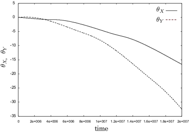
Figure 2: The time evolution of $\theta_{X}(t)$ and $\theta_{Y}(t)$ is plotted in the case of the quasi-spin squeezed state approach. The parameters are taken as $G=1.2$, $\epsilon=1.0$ and $\Omega=2N=8$. The initial values are $n_{X}(t=0)=1.3$, $\theta_{X}(t=0)=0.0$, $n_{Y}(t=0)=0.35$ and $\theta_{Y}(t=0)=0.0$.

On the other hand, in the quasi-spin squeezed state approximation, the equations of motion derived from (34) are written as

$$\dot{\theta_{X}} = \frac{\partial H_{\rm sq}}{\partial n_{X}}$$

$$= 2\epsilon-2GS_{j}\left\{\frac{\partial{\cal X}}{\partial n_{X}}+\frac{n_{X}}{S_{j}(2S_{j}-4n_{Y})}+\frac{4}{S_{j}^{2}}\cdot\frac{\partial{\cal X}}{\partial n_{X}}\cdot{\cal Y}\cdot[n_{Y}+n_{Y}^{2}L-n_{Y}^{2}]\right.$$

$$\qquad\qquad\ \ \left.-\frac{2}{S_{j}}\sqrt{n_{Y}K}\cdot\frac{\partial{\cal X}}{\partial n_{X}}\cos(2\theta_{X}-\theta_{Y})-2\cdot\frac{\partial{\cal X}}{\partial n_{X}}\frac{{\cal Y}}{S_{j}}\cdot L\right\}\ ,$$

$$\dot{n_{X}} = -\frac{\partial H_{\rm sq}}{\partial\theta_{X}}=8G\sqrt{n_{Y}K}~{}\!{\cal X}{\cal Y}\sin(2\theta_{X}-\theta_{Y})\ ,$$ (38)

$$\dot{\theta_{Y}} = \frac{\partial H_{\rm sq}}{\partial n_{Y}}$$

$$= 4\epsilon-2GS_{j}\left\{\frac{\partial{\cal X}}{\partial n_{Y}}+\frac{n_{X}^{2}\cdot{\cal Y}}{2S_{j}^{3}}~{}\!+~{}\!\frac{4}{S_{j}^{2}}\cdot\left[\frac{\partial{\cal X}}{\partial n_{Y}}{\cal Y}+\frac{\partial{\cal Y}}{\partial n_{Y}}{\cal X}\right]\cdot{\cal Y}\cdot[n_{Y}+n_{Y}^{2}L-n_{Y}^{2}]\right.$$

$$\qquad\qquad+\frac{4}{S_{j}^{2}}\cdot{\cal X}{\cal Y}\cdot[1+2n_{Y}L+n_{Y}^{2}\frac{\partial L}{\partial n_{Y}}-2n_{Y}]$$

$$\qquad\qquad-\frac{1}{S_{j}\sqrt{n_{Y}K}}(K+n_{Y}\frac{\partial K}{\partial n_{Y}}){\cal X}{\cal Y}\cos(2\theta_{X}-\theta_{Y})$$

$$\qquad\qquad-\frac{2}{S_{j}}\sqrt{n_{Y}K}\left[\frac{\partial{\cal X}}{\partial n_{Y}}{\cal Y}+\frac{\partial{\cal Y}}{\partial n_{Y}}{\cal X}\right]\cos(2\theta_{X}-\theta_{Y})$$

$$\qquad\qquad-\frac{2}{S_{j}}\left[\frac{\partial{\cal X}}{\partial n_{Y}}{\cal Y}+\frac{\partial{\cal Y}}{\partial n_{Y}}{\cal X}\right]\cdot\left[\left(1-\frac{1}{2S_{j}}\right)n_{Y}-\frac{n_{Y}^{2}}{S_{j}}L\right]$$

$$\qquad\qquad\left.+2\left[1-\frac{{\cal X}{\cal Y}}{S_{j}}\right]\cdot\left[\left(1-\frac{1}{2S_{j}}\right)-\frac{1}{S_{j}}\left[2n_{Y}L+n_{Y}^{2}\frac{\partial L}{\partial n_{Y}}\right]\right]\right\}\ ,$$

$$\dot{n_{Y}} = -\frac{\partial H_{sq}}{\partial\theta_{Y}}=-4G\sqrt{n_{Y}K}~{}\!{\cal X}{\cal Y}~{}\!\sin(2\theta_{X}-\theta_{Y})$$ (39)

Here, the number conservation is satisfied:

$${\dot{N}}=2{\dot{n}_{X}}+4{\dot{n}_{Y}}=0\ .$$ (40)

The time evolution of $n_{X}(t)$ and $n_{Y}(t)$ in Fig.2 and $\theta_{X}(t)$ and $\theta_{Y}(t)$ in Fig.2 is plotted with appropriate initial conditions. The parameters used here are $G=1.2$, $\epsilon=1.0$ and $\Omega=2N=8$. In the $su(2)$-coherent state approach, $n_{X}$ is constant of motion. However, quasi-spin squeezed state approach, $n_{X}$ and $n_{Y}$ oscillate with antiphase, while the total particle number is conserved.

4 Dynamical approach to the ground state energy

Hereafter, we assume that $|Y|^{2}\ (=n_{Y})\ll 1$ because $|Y|^{2}$ means the quantum fluctuations. Then, $K(Y^{*}Y)$ and $L(Y^{*}Y)$ defined in (24) and (25e), respectively, can be evaluated by the expansion with respect to $|Y|^{2}$. As a result, we obtain

$$K(Y^{*}Y) = \frac{1}{2}\left(1-\frac{1}{2S_{j}}\right)+\left(1-\frac{7}{2S_{j}}+\frac{9}{(2S_{j})^{2}}\right)Y^{*}Y+\cdots\ .$$

$$L(Y^{*}Y) = \frac{1}{1-\frac{1}{2S_{j}}}3\left(1-\frac{2}{2S_{j}}\right)\!\!\left(1-\frac{3}{2S_{j}}\right)$$ (41)

$$-\frac{48}{2S_{j}}\frac{1}{(1-\frac{1}{2S_{j}})^{2}}\left(1-\frac{2}{2S_{j}}\right)\!\!\left(1-\frac{3}{2S_{j}}\right)\!\!\left(1-\frac{4}{2S_{j}}\right)Y^{*}Y+\cdots\ .\qquad$$

Then, the expectation values for the Hamiltonian, the time-derivative and the number operator can be expressed as

$$H_{\rm sq}=\epsilon(2n_{X}+4n_{Y})-G\biggl{[}2S_{j}n_{X}-n_{X}^{2}+\frac{n_{X}^{2}}{2S_{j}}$$

$$\qquad\quad-2\sqrt{2}\sqrt{1-\frac{1}{2S_{j}}}\left(1-\frac{n_{X}}{2S_{j}}\right)n_{X}\sqrt{n_{Y}}\cos(2\theta_{X}-\theta_{Y})$$

$$\qquad\quad+2\left(2S_{j}-1-4n_{X}+\frac{10}{2S_{j}}n_{X}+\frac{2}{2S_{j}}n_{X}^{2}-\frac{8}{(2S_{j})^{2}}n_{X}^{2}\right)n_{Y}+{\rm O}(n_{Y}^{3/2})\biggl{]}\ ,$$

(42a)

$$\langle{\psi(\alpha,\beta)}|i\partial_{t}|{\psi(\alpha,\beta)}\rangle=(n_{X}{\dot{\theta}}_{X}+n_{Y}{\dot{\theta}}_{Y})\ ,$$ (42b)

$$N=\langle{\psi(\alpha,\beta)}|{\hat{N}}|{\psi(\alpha,\beta)}\rangle=2n_{X}+4n_{Y}\ .$$ (42c)

From the time-dependent variational principle (34) or (38) and (39), the following equations of motion are derived under the above-mentioned approximation :

$${\dot{\theta}}_{X}=\frac{\partial H_{\rm sq}}{\partial n_{X}}\approx 2\epsilon-G\!\cdot\!2\biggl{[}S_{j}\!-\!n_{X}\!+\!\frac{n_{X}}{2S_{j}}\!-\!\sqrt{2}\sqrt{1-\frac{1}{2S_{j}}}\!\!\left(1-\frac{n_{X}}{S_{j}}\right)\!\!\sqrt{n_{Y}}\cos(2\theta_{X}-\theta_{Y})$$

$$\qquad\qquad\qquad\qquad\qquad+4\left(-1+\frac{5}{4S_{j}}+\frac{1}{2S_{j}}n_{X}-\frac{1}{S_{j}^{2}}n_{X}\right)n_{Y}\biggl{]}\ ,$$ (43a)

$${\dot{n}}_{X}=-\frac{\partial H_{\rm sq}}{\partial\theta_{X}}\approx-G\cdot 4\sqrt{2}\sqrt{1-\frac{1}{2S_{j}}}\!\left(1-\frac{n_{X}}{2S_{j}}\right)\!n_{X}\sqrt{n_{Y}}\sin(2\theta_{X}-\theta_{Y})\ ,$$ (43b)

$${\dot{\theta}}_{Y}=\frac{\partial H_{\rm sq}}{\partial n_{Y}}\approx 4\epsilon-G\biggl{[}-\sqrt{2}\sqrt{1-\frac{1}{2S_{j}}}\!\!\left(1-\frac{n_{X}}{2S_{j}}\right)\!\!\frac{n_{X}}{\sqrt{n_{Y}}}\cos(2\theta_{X}-\theta_{Y})$$

$$\qquad\qquad\qquad\qquad\qquad+2\left(-1+2S_{j}-4n_{X}+\frac{5}{S_{j}}+\frac{1}{S_{j}}n_{X}^{2}-\frac{2}{S_{j}^{2}}n_{X}^{2}\right)\biggl{]}\ ,$$ (43c)

$${\dot{n}}_{Y}=-\frac{\partial H_{\rm sq}}{\partial\theta_{Y}}\approx G\cdot 2\sqrt{2}\sqrt{1-\frac{1}{2S_{j}}}\!\left(1-\frac{n_{X}}{2S_{j}}\right)\!n_{X}\sqrt{n_{Y}}\sin(2\theta_{X}-\theta_{Y})\ .$$ (43d)

It is found from (43b) and (43d) that the total fermion number $N$ in (42c) is also conserved in this approximation, that is,

$${\dot{N}}=2{\dot{n}}_{X}+4{\dot{n}}_{Y}=0\ .$$ (44)

It should be noted here that $n_{X}\leq N/2$ from (42c) and $N\leq\Omega/2=S_{j}$. Thus, the inequality $1-n_{X}/2S_{j}\geq 0$ is obtained. From the approximated energy expectation value (42a) for $G>0$, the energy minimum is then obtained in the case $\cos(2\theta_{X}-\theta_{Y})=-1$, namely,

$$\theta_{Y}=2\theta_{X}+\pi\ .$$ (45)

Since the energy is minimal in the ground state, the relation (45) should be satisfied at any time. In order to assure the above-mentioned situation, the following consistency condition should be obeyed :

$${\dot{\theta}}_{Y}=2{\dot{\theta}}_{X}\ .$$ (46)

Thus, from the equations of motion (43a) and (43c), under the approximation of small $n_{Y}$, the consistency condition (46) gives the following expression of $n_{Y}$ in the lowest order approximation of $n_{Y}$ :

$$\sqrt{n_{Y}} \approx \frac{\sqrt{1-\frac{1}{2S_{j}}}}{2\sqrt{2}(1-\frac{2}{S_{j}})}\cdot\left[1+\frac{1}{2n_{X}}\frac{1}{(1-\frac{n_{X}}{2S_{j}})(1-\frac{2}{S_{j}})}\right]^{-1}\ .$$ (47)

Thus, by substituting (45) and $\sqrt{n_{Y}}$ in (47) under the lowest order approximation of $n_{Y}$ into the energy expectation value (42a), and by performing the approximation of large $N$ or large $\Omega(=2S_{j})$ approximation, we obtain the ground state energy as

$$H_{\rm sq}=\epsilon N-\frac{1}{4}GN\Omega\left(2-\frac{N}{\Omega}+\frac{2}{\Omega}+{\rm O}(1/(N\Omega),1/\Omega^{2},1/N^{2})\right)\ .$$ (48)

This result reproduces the exact energy eigenvalue (6) by neglecting the higher order term of $1/(N\Omega)$, $1/\Omega^{2}$ and $1/N^{2}$ for large $N$ and $\Omega$ limit. Thus, the quasi-spin squeezed state presents a good approximation in the time-dependent variational approach to the pairing model. In this approach, the existence of the rotational motion in the phase space consisting of $(n_{X},\theta_{X};n_{Y},\theta_{Y})$ plays the important role. The angle variables for rotational motion, $\theta_{X}$ and $\theta_{Y}$, are consistently changed in (46). This consistency condition is essential to reproduce the exact energy for the ground state under the large $N$ and $\Omega$ limit. The approximation corresponds to so-called large $N$ approximation. In general, it is known that the large $N$ expansion at zero temperature corresponds to $\hbar$ expansion. In this sense, the time-dependent variational approach with the quasi-spin squeezed state gives the approximation including the higher order quantum fluctuations than $\hbar$ if any expansion is not applied.

5 Summary

In this paper, it has been shown that the exact ground state energy for the pairing model can be well recovered by using the time-dependent variational approach with the quasi-spin squeezed state. For this purpose, we treated the $su(2)$-algebraic model because its eigenvalue is known analytically. As a result, by taking into account of the dynamics in our quasi-spin squeezed state approach, the exact ground state energy can be reproduced up to the order of $1/\Omega$ under the small $|Y|^{2}$ expansion. Of course, the time evolution of a system governed by the pairing model Hamiltonian can be also investigated as is similar to that of the Lipkin model developed in Ref.TA04. However, we do not repeat it because the result is almost same as that of the Lipkin model, which was reported in Ref.TA04.

References

[1]
Y. Tsue and H. Akaike,
Prog. Theor. Phys. 113 (2005), 105.
[2]
Y. Tsue, A. Kuriyama and M. Yamamura, Prog. Theor. Phys.
92 (1994), 545.
[3]Y. Tsue, N. Azuma, A. Kuriyama and M. Yamamura,
Prog. Theor. Phys. 96 (1996), 729.
[4]A. Kuriyama, J. da Providência, Y. Tsue and M. Yamamura,
Prog. Theor. Phys. Suppl. 141 (2001), 113.
[5]
H. Akaike, Y. Tsue and S. Nishiyama,
Prog. Theor. Phys. 112 (2004), 583.
[6]
A. K. Kerman, Ann. of Phys. 12 (1961), 300.
[7]
R. D. Lawson and M. H. Macfarlane, Nucl. Phys. 66 (1965), 80.
[8]
See, for example, J. M. Eisenberg and W. Greiner, Nuclear Theory Vol.3.
[9]
M. Yamamura and A. Kuriyama, Prog. Theor. Phys. Suppl. No.93 (1987), 1.
[10]
M. Yamamura, private communication (unpublished work).