Using chiral perturbation theory to extract the neutron-neutron scattering length from $\pi^{-}d\to nn\gamma$

Abstract

The reaction $\pi^{-}d\to nn\gamma$ is calculated in chiral perturbation theory so as to facilitate an extraction of the neutron-neutron scattering length ($a_{nn}$). We include all diagrams up to $O(Q^{3})$. This includes loop effects in the elementary $\pi^{-}p\to\gamma n$ amplitude and two-body diagrams, both of which were ignored in previous calculations. We find that the chiral expansion for the ratio of the quasi-free (QF) to final-state-interaction (FSI) peaks in the final-state neutron spectrum converges well. Our third-order calculation of the full spectrum is already accurate to better than 5%. Extracting $a_{nn}$ from the shape of the entire $\pi^{-}d\to nn\gamma$ spectrum using our calculation in its present stage would thus be possible at the $\pm 0.8$ fm level. A fit to the FSI peak only would allow an extraction of $a_{nn}$ with a theoretical uncertainty of $\pm 0.2$ fm. The effects that contribute to these error bars are investigated. The uncertainty in the $nn$ rescattering wave function dominates. This suggests that the quoted theoretical error of $\pm 0.3$ fm for the most recent $\pi^{-}d\to nn\gamma$ measurement may be optimistic. The possibility of constraining the $nn$ rescattering wave function used in our calculation more tightly—and thus reducing the error—is briefly discussed.

I Introduction

In QCD, charge symmetry (CS) is a symmetry of the Lagrangian under the exchange of the up and down quarks MNS . This symmetry has many consequences at the hadronic level, where it translates into, e.g., the invariance of the strong nuclear force under the exchange of protons and neutrons. However, CS is broken by the different masses of the up and down quarks and thus the strong interaction manifests charge symmetry breaking (CSB). The different electromagnetic properties of the up and down quarks also contribute to CSB. An important consequence of the first CSB effect (strong CSB) is that the neutron is heavier than the proton, since if CSB was only an electromagnetic effect the proton would be heavier and prone to decay. This would make our world very different, since big-bang nucleosynthesis is dependent on the relative proton and neutron abundances.

While there are a number of pieces of experimental evidences for CSB MNS —including recent results in $dd\to\alpha\pi^{0}$ at IUCF IUCFCSB and $np\to d\pi^{0}$ at TRIUMF Allena —one of the most fundamental to nuclear physics is the difference between the neutron-neutron ($a_{nn}$) and proton-proton ($a_{pp}$) scattering lengths. The scattering lengths parameterize the nucleon-nucleon interaction at low relative energies through the effective range expansion. In this low-energy region the (${}^{1}S_{0}$) phase shift $\delta_{0}$ can be expressed as

$$p\cot\delta_{0}=-\frac{1}{a}+\frac{1}{2}r_{0}p^{2},$$ (1)

where $p$ is the center-of-momentum (c.m.) relative nucleon momentum and $r_{0}$ the effective range. This expansion is reliable for $p\lesssim 150$ MeV/$c$.

Since there are no free neutron targets it is very difficult to make a direct measurement of the ${}^{1}S_{0}$ neutron-neutron scattering length, though proposals to do so have been made. The latest of these suggests using the pulsed nuclear reactor YAGUAR in Snezhinsk, Russia yaguar . However, the more common—and so far more successful—approach is to rely on suitable reactions involving two free neutrons and corresponding theoretical calculations to extract $a_{nn}$ from indirect data. By choosing the kinematics carefully one can detect the neutrons in a low-energy relative $S$-wave which can be accurately described by the effective range expansion (1). The currently accepted value

$$a_{nn}=-18.5\pm 0.3\ {\rm fm}$$ (2)

is deduced from the break-up reaction $nd\to nnp$ and the pion radiative capture process $\pi^{-}d\to nn\gamma$. The first reaction is, however, complicated by the possible presence of three-body forces, but even after they are taken into account there are significant disagreements between values extracted by the two techniques. A recent $nd$ break-up experiment reports $a_{nn}=-16.1\pm 0.4$ fm nd1 , i.e., more than five standard deviations from the standard value (2). The result of Ref. nd1 is also in disagreement with another $nd$ experiment that claims $-18.7\pm 0.6$ fm nd2 . Earlier data had an even larger spread, see Ref. Slaus for a review. Since the proton-proton scattering length is $a_{pp}=-17.3\pm 0.4$ fm (after corrections of electromagnetic effects ), there is even uncertainty about the sign of the difference $a_{pp}-a_{nn}$. The more negative $a_{nn}$ is favored by nuclear structure calculations, where the small (but important) CSB piece of the AV18 potential is fitted to reproduce $a_{pp}-a_{nn}$ with $a_{nn}=-18.5$ fm Wi95 . The binding-energy difference between ${}^{3}{\rm H}$ and ${}^{3}{\rm He}$, which has a small contribution from CSB effects, is then very accurately reproduced. This would not occur were $a_{pp}-a_{nn}$ to take the opposite sign AV18 .

Because of these issues the accepted value is weighted toward the $a_{nn}=-18.50\pm 0.05(\rm stat.)\pm 0.44(syst.)\pm 0.30(theory)$ fm reported by the most recent $\pi^{-}d\to nn\gamma$ experiment LAMPF . The extraction in this is case done by fitting the shape of the neutron time-of-flight spectrum using the model of Gibbs, Gibson, and Stephenson (GGS) GGS . This model was developed in the mid-70s and explored many of the relevant mechanisms and the dependence on various choices of wave functions. Gibbs, Gibson, and Stephenson calculated the single-nucleon radiative pion capture tree-level amplitude to order $p/M$, and consequently ignored the pion loops that would enter at the next chiral order. Two-body diagrams were not fully implemented in this model. The theoretical error was dominated by uncertainties in the scattering wave function. Similar results were obtained in earlier $\pi^{-}d\to nn\gamma$ experiments carried out at the Paul Scherrer Institut (PSI) (then Swiss Institute of Nuclear Research) Gabioudetal . In the PSI experiments, only the FSI peak was fitted, while at LAMPF the entire spectrum was fitted. The theoretical work for the PSI results compared the GGS model with work done by de Téramond and collaborators deTeramond . The latter used a dispersion relation approach for the final state interaction, with a theoretical error of the order 0.3 fm, i.e., similar to GGS.

In this paper we recalculate the $\pi^{-}d\to nn\gamma$ reaction using chiral perturbation theory ($\chi$PT). The one-body and two-body mechanisms are thus consistent and the constraints of chiral symmetry are respected, which is of crucial importance in this threshold regime. At third order, $O(Q^{3})$, all the amplitudes of the previous calculation are included, as well as pion loops and three pion-rescattering diagrams. Additional advantages of the chiral power counting are that it gives a clearly defined procedure to estimate the theoretical error and provides a systematic and consistent way to improve the calculation if needed. In this first paper we establish the machinery necessary for a precise extraction of the $nn$ scattering length. We isolate the sources of the largest remaining errors and suggest means for their reduction, which should make it possible to reach the desired high precision in future work.

The paper is organized as follows. In Sec. II we will develop the main ingredients of our calculation: the Lagrangian, the explicit forms of the one- and two-body amplitudes, and a description of our wave functions. The numerical results are presented in Sec. III together with our estimate of the theoretical error. We conclude in Sec. IV.

II Layout of calculation

The LAMPF experiment LAMPF used stopped pions, captured into atomic orbitals around the deuteron. The subsequent radiative decay occurs for pionic $s$-wave orbitals only. Thus the c.m. and laboratory frames coincide and the pion momentum is vanishingly small. The neutron time-of-flight distribution of the c.m. $\pi^{-}d$ decay width (with the photon and one neutron detected) can be expressed as

$$\frac{d^{2}\Gamma}{dt_{1}d\theta_{3}}=\frac{1}{2(2\pi)^{3}M_{\pi d}t_{1}}\frac{p_{1}^{3}E_{1}k\sin\theta_{3}}{M_{\pi d}-E_{1}-p_{1}\cos\theta_{3}}\frac{1}{3}\sum_{\rm pols.}|\mathcal{M}|^{2},$$ (3)

where $t_{1}$, $p_{1}$, and $E_{1}$ are the time-of-flight, momentum, and energy of the detected neutron, $\theta_{3}$ is the supplement of the angle between this neutron and the photon, and $k$ is the photon momentum. Here the sum is over deuteron and photon polarizations and $M_{\pi d}$ is the mass of the deuteron-pion bound system, which to a very good approximation is given by the sum of the pion ($\mu$) and deuteron ($M_{d}$) masses.

The matrix element $\mathcal{M}$ is the sum of four interfering parts, the quasi-free (QF) one-body, the one-body with final state interaction (FSI), and the two-body contributions, with and without FSI. These can be symbolized by the generic diagrams shown in Fig. 1. In this first calculation we restrict FSI to $S$-waves only, and subtract the plane-wave from the scattering wave function and include it in the QF contribution.

Figure 1: Generic diagrams of the contributions to $\pi^{-}d\to nn\gamma$. Diagram (a) and (b) are the one-body contributions, without and with FSI. Diagram (c) and (d) are the corresponding for the two-body currents. The amplitudes $\mathcal{A}_{\rm I}$ and $\mathcal{A}_{\rm II}$ are described in the text.

We will derive the matrix elements for $\gamma nn\to\pi^{-}d$ rather than $\pi^{-}d\to nn\gamma$ in order to reduce the possibility of relative phase errors when using the $\gamma n\to\pi^{-}p$ amplitudes. The $\pi^{-}d\to nn\gamma$ decay rate can of course then be obtained by detailed balance. An explicit expression for the matrix element in terms of $\pi d$ atomic ($\Phi_{\pi d}$) and deuteron ($\varphi_{d}$) wave functions and the pion-photon amplitude $\mathcal{A}$ is given by

$$\mathcal{M}(\gamma nn\to\pi^{-}d) = \int\frac{d^{3}qd^{3}p^{\prime}d^{3}p^{\prime\prime}}{(2\pi)^{9}}\frac{M\sqrt{2E_{\pi d}}}{\sqrt{E_{1}E_{2}2E_{\pi}}}\Phi^{\ast}_{\pi d}(0;{\bf q})\varphi^{\ast}_{d}(-{\bf q};{\bf p}^{\prime\prime})\mathcal{A}\Psi_{\bf-k}({\bf p}^{\prime},{\bf p}),$$ (4)

where ${\bf p}$, ${\bf p}^{\prime}$, and ${\bf p}^{\prime\prime}$ are the initial, intermediate, and final relative momenta of the two nucleons (for $\gamma nn\to\pi^{-}d$), while ${\bf q}$ is the pion c.m. momentum and $E_{x}$ the energy of the indicated particle. The meaning of these kinematic variables can also be inferred from Fig. 2.

Figure 2: Basic diagram for $\pi^{-}d\to nn\gamma$, defining kinematic variables.

Here $\Psi_{\bf-k}({\bf p}^{\prime},{\bf p})$ is the $nn$ scattering wave function at total momentum ${\bf-k}$, normalized such that

$$\int\frac{d^{3}q}{(2\pi)^{3}}\Psi^{\ast}_{\bf-k}({\bf p}^{\prime},{\bf q})\Psi_{\bf-k}({\bf p},{\bf q})=(2\pi)^{3}\delta^{3}({\bf p}^{\prime}-{\bf p}).$$ (5)

Its Fourier transform is given by

$$\Psi_{\bf-k}({\bf p}^{\prime},{\bf p})=\int\frac{d^{3}r}{(2\pi)^{3}}e^{-i{\bf p}^{\prime}\cdot{\bf r}}\Psi_{\bf-k}({\bf r},{\bf p}),$$ (6)

where $\Psi_{\bf-k}({\bf p},{\bf r})=\sum_{l}(2l+1)i^{l}\frac{v_{l}(r)}{r}P_{l}(\mbox{\boldmath${\widehat{\bf p}}$}\cdot\mbox{\boldmath${\widehat{\bf r}}$})$, which could be compared to the plane wave expansion $e^{i{\bf p}\cdot{\bf r}}=\sum_{l}(2l+1)i^{l}j_{l}(pr)P_{l}(\mbox{\boldmath${\widehat{\bf p}}$}\cdot\mbox{\boldmath${\widehat{\bf r}}$})$. The form of $v_{l}(r)$ will be discussed in Sec. II.5.

The pion-photon amplitude $\mathcal{A}$ can be separated into the one- and two-body amplitudes $\mathcal{A}_{\rm I}$ and $\mathcal{A}_{\rm II}$;

$$\mathcal{A} = (2\pi)^{3}\frac{E}{M}\delta^{(3)}(\tilde{\bf p}\pm\frac{{\bf k}-{\bf q}}{2})\mathcal{A}_{\rm I}({\bf k},{\bf q})+\mathcal{A}_{\rm II}(\pm\tilde{\bf p},{\bf k},{\bf q}),$$ (7)

where the upper(lower) sign is for interaction on nucleon 1(2) of the deuteron and $\tilde{\bf p}={\bf p}^{\prime}-{\bf p}^{\prime\prime}$. The one- and two-body matrix elements are then

$$\mathcal{M}_{\rm I}(\gamma nn\to\pi^{-}d) = \int\frac{d^{3}qd^{3}p^{\prime}}{(2\pi)^{6}}\frac{E\sqrt{2E_{\pi d}}}{\sqrt{E_{1}E_{2}2E_{\pi}}}\Phi^{\ast}_{\pi d}(0;{\bf q})\varphi^{\ast}_{d}(-{\bf q};{\bf p}^{\prime}\pm\frac{\bf k-q}{2})\mathcal{A}_{\rm I}({\bf k},{\bf q})\Psi_{-\bf k}({\bf p}^{\prime},{\bf p}),$$

$$\mathcal{M}_{\rm II}(\gamma nn\to\pi^{-}d) = \int\frac{d^{3}qd^{3}p^{\prime}d^{3}p^{\prime\prime}}{(2\pi)^{9}}\frac{M\sqrt{2E_{\pi d}}}{\sqrt{E_{1}E_{2}2E_{\pi}}}\Phi^{\ast}_{\pi d}(0;{\bf q})\varphi^{\ast}_{d}(-{\bf q};{\bf p}^{\prime\prime})\mathcal{A}_{\rm II}(\pm\tilde{\bf p},{\bf k},{\bf q})$$ (8)

$$\times \Psi_{-\bf k}({\bf p}^{\prime},{\bf p}).$$

In configuration space the matrix elements are given by

$$\mathcal{M}_{\rm I}^{\rm FSI} = \sum\Phi_{\pi d}(0)\sqrt{\frac{M_{\pi d}}{\mu}}\int dr\frac{d\Omega_{r}}{\sqrt{4\pi}}[S_{0}u(r)+S_{2}(\mbox{\boldmath${\widehat{\bf r}}$})w(r)]e^{\pm\frac{i}{2}({\bf k}-{\bf q})\cdot{\bf r}}\mathcal{A}_{\rm I}({\bf k},{\bf q})\tilde{v}_{0}(r)\chi_{0},$$ (9)

$$\mathcal{M}_{\rm I}^{\rm QF} = \sum\Phi_{\pi d}(0)\sqrt{\frac{M_{\pi d}}{\mu}}\int rdr\frac{d\Omega_{r}}{\sqrt{4\pi}}[S_{0}u(r)+S_{2}(\mbox{\boldmath${\widehat{\bf r}}$})w(r)]e^{\pm\frac{i}{2}({\bf k}-{\bf q})\cdot{\bf r}}\mathcal{A}_{\rm I}({\bf k},{\bf q})e^{i{\bf p}\cdot{\bf r}}\chi_{S},$$ (10)

$$\mathcal{M}_{\rm II}^{\rm FSI} = \sum\Phi_{\pi d}(0)\sqrt{\frac{M_{\pi d}}{\mu}}\int dr\frac{d\Omega_{r}}{\sqrt{4\pi}}[S_{0}u(r)+S_{2}(\mbox{\boldmath${\widehat{\bf r}}$})w(r)]\mathcal{A}^{\pm}_{\rm II}({\bf r},{\bf k},{\bf q})\tilde{v}_{0}(r)\chi_{0},$$ (11)

$$\mathcal{M}_{\rm II}^{\rm PW} = \sum\Phi_{\pi d}(0)\sqrt{\frac{M_{\pi d}}{\mu}}\int rdr\frac{d\Omega_{r}}{\sqrt{4\pi}}[S_{0}u(r)+S_{2}(\mbox{\boldmath${\widehat{\bf r}}$})w(r)]\mathcal{A}^{\pm}_{\rm II}({\bf r},{\bf k},{\bf q})e^{\pm i{\bf p}_{i}\cdot{\bf r}}\chi_{S},$$ (12)

where ${\bf p}_{1,2}=-\frac{1}{2}{\bf k}\pm{\bf p}$, $\mathcal{A}^{\pm}_{\rm II}({\bf r},{\bf k},{\bf q})=\int\frac{d^{3}\tilde{p}}{(2\pi)^{3}}e^{-i\tilde{\bf p}\cdot{\bf r}}\mathcal{A}_{\rm II}(\pm\tilde{\bf p},{\bf k},{\bf q})$, and $\tilde{v}_{0}(r)$ is the subtracted scattering wave function as defined in Sec. II.5. The sums are over the two nucleons. In these expressions $\Phi_{\pi d}(0)=(\mu_{\pi d}\alpha)^{3/2}/\sqrt{\pi}$ is the pion-deuteron atomic $s$-orbital wave function evaluated at the origin with $\mu_{\pi d}$ the reduced $\pi d$ mass, while $S_{0}=-\frac{1}{\sqrt{2}}\mbox{\boldmath${\sigma}$}\cdot\mbox{\boldmath${\epsilon}$}_{d}^{\dagger}$ and $S_{2}(\mbox{\boldmath${\widehat{\bf r}}$})=\frac{1}{2}(3\mbox{\boldmath${\sigma}$}\cdot\mbox{\boldmath${\widehat{\bf r}}$}\,\mbox{\boldmath${\widehat{\bf r}}$}\cdot\mbox{\boldmath${\epsilon}$}_{d}^{\dagger}-\mbox{\boldmath${\sigma}$}\cdot\mbox{\boldmath${\epsilon}$}_{d}^{\dagger})$ are the $S$- and $D$-wave spin structures of the deuteron, $\mbox{\boldmath${\epsilon}$}_{d}^{\dagger}$ being the deuteron polarization vector. The $\chi_{S}$’s are the neutron-neutron spin wave functions for spin $S$.

In the following subsections we will derive explicit expressions for the amplitudes and show how the coordinate-space wave functions are obtained.

II.1 Power counting

We start from the relativistic Lagrangian

$$\mathcal{L} = {\cal L}_{\pi N}^{(1)}+{\cal L}_{\pi N}^{(2)}+{\cal L}_{\pi\pi}^{(2)};$$

$${\cal L}_{\pi N}^{(1)} = \bar{N}\left[i\gamma\cdot D_{N}-M-\frac{1}{4f_{\pi}^{2}}\epsilon^{abc}\tau^{c}\pi^{a}\gamma\cdot\partial\pi^{b}-\frac{g_{A}}{2f_{\pi}}(\gamma\cdot D^{ab}\pi^{a})\tau^{b}\gamma_{5}\right]N,$$

$${\cal L}_{\pi N}^{(2)} = -\bar{N}\left[\frac{e(\kappa_{0}+\kappa_{1}\tau^{3})}{8M}\sigma^{\mu\nu}F_{\mu\nu}\right]N,$$

$${\cal L}_{\pi\pi}^{(2)} = \frac{1}{2}D_{\mu}^{ab}\pi^{a}D^{\mu cb}\pi^{c}-\frac{1}{2}\mu^{2}\mbox{\boldmath${\pi}$}^{2},$$ (13)

where $D^{\mu}_{N}=\partial^{\mu}-ieQ_{N}A^{\mu}$ and $D^{\mu ab}_{\pi}=\delta^{ab}\partial^{\mu}-ieQ^{ab}_{\pi}A^{\mu}$ are the covariant derivatives for the nucleon and pion ($e<0$), $Q_{N}=\frac{1}{2}(1+\tau^{3})$ and $Q^{ab}_{\pi}=i\epsilon^{ab3}$ are the electric charge isospin operators (with $a$/$b$ isospin indices of incoming/outgoing pion), and $\kappa_{0,1}=\kappa_{p}\pm\kappa_{n}$ ($\kappa_{p}=1.793$ and $\kappa_{n}=-1.913$) represent the nucleon anomalous magnetic moments. The electromagnetic field tensor is given by $F_{\mu\nu}=\partial_{\nu}A_{\mu}-\partial_{\mu}A_{\nu}$ and $\sigma^{\mu\nu}=\frac{i}{2}[\gamma^{\mu},\gamma^{\nu}]$ as usual.

The Lagrangian (13) is organized according to the number of powers of small momenta $Q$ (here $e$ counts as one “small” momentum). The chiral order of any graph to any amplitude involving nucleons, together with pions and photons with energies of order $\mu$ can be assessed by multiplying the $Q$-scaling factors of the individual units of the graph by one another. These factors are as follows:

• Each vertex from ${\cal L}^{(n)}$ contributes $Q^{n}$.

• Each nucleon propagator scales like $1/Q$ (provided that the energy flowing through the nucleon line is $\sim\mu$);

• Each pion propagator scales like $1/Q^{2}$;

• Each pion loop contributes $Q^{4}$;

• Graphs in which two nucleons participate in the reaction acquire an extra factor of $Q^{3}$.

In practice tree-level relativistic graphs must be calculated, and then expanded in powers of $p/M$ in order to establish contact with the usual heavy-baryon formulation of chiral perturbation theory. The expressions for loop graphs that we use are also computed in heavy-baryon $\chi$PT, and so we do not need to employ any special subtraction schemes to remove pieces of loop integrals which scale with positive powers of the nucleon mass BL99 ; Fu03 .

Note that we will employ the Coulomb gauge in all calculations.

II.2 One-body amplitudes

There are four basic one-body diagrams, shown in Fig. 3: the Kroll-Ruderman (KR) term (a), the pion pole (b), and the $s$- and $u$-channel nucleon pole terms (c) and (d).

Figure 3: Single-nucleon pion-photon diagrams relevant for pion photoproduction. In this and all other figures a solid line represent a nucleon, a dashed line a pion and a wavy line a photon.

They can be calculated directly from a non-relativistic reduction of the relativistic Lagrangian or from the amplitudes of heavy-baryon $\chi$PT (HB$\chi$PT) ulfreview . In addition, there are also pion-loop corrections at $O(Q^{3})$ as shown in Fig. 4.

Figure 4: Pion loops at NNLO for $\gamma N\to\pi N$ in Coulomb gauge. Note that not all time orderings are shown.

The loop corrections, together with the corresponding counterterms from ${\cal L}_{\pi N}^{(3)}$ EM have already been calculated in the $\gamma N$ c.m. frame to $O(Q^{3})$ for radiative pion capture on a nucleon Fearing using Coulomb gauge. The low-energy constants (LECs) from the third-order chiral Lagrangian were fitted to experiment, yielding an excellent description of the near-threshold data.

The third-order piece of the one-body amplitudes of Ref. Fearing can hence be taken as is, without introducing any new unknown parameters, and combined with our evaluation to $O(Q^{2})$ of the tree-level diagrams in Fig. 3 using the relativistic Lagrangian (13) . In order to incorporate these amplitudes in the two-body system they should be evaluated at the relevant subthreshold kinematics, corrected for a boost to the overall rest frame, and corrected for off-shell effects. These issues will all be discussed below.

The full one-body amplitude is given (in Coulomb gauge) by

$$\mathcal{A}_{\rm I}(\gamma N\to\pi N) = F_{1}(E_{\pi},x)i\mbox{\boldmath${\sigma}$}\cdot\mbox{\boldmath${\epsilon}$}_{\gamma}+F_{2}(E_{\pi},x)\mbox{\boldmath${\sigma}$}\cdot\mbox{\boldmath${\widehat{\bf q}}$}\,\mbox{\boldmath${\sigma}$}\cdot(\mbox{\boldmath${\widehat{\bf k}}$}\times\mbox{\boldmath${\epsilon}$}_{\gamma})+F_{3}(E_{\pi},x)i\mbox{\boldmath${\sigma}$}\cdot\mbox{\boldmath${\widehat{\bf k}}$}\,\mbox{\boldmath${\widehat{\bf q}}$}\cdot\mbox{\boldmath${\epsilon}$}_{\gamma}$$ (14)

$$+ F_{4}(E_{\pi},x)i\mbox{\boldmath${\sigma}$}\cdot\mbox{\boldmath${\widehat{\bf q}}$}\,\mbox{\boldmath${\widehat{\bf q}}$}\cdot\mbox{\boldmath${\epsilon}$}_{\gamma},$$

where the $F_{i}$ are the Chew-Goldberger-Low-Nambu (CGLN) amplitudes CGLN and $\mbox{\boldmath${\epsilon}$}_{\gamma}$ is the photon polarization vector. The isospin channels are separated as

$$F_{i}^{a}(E_{\pi},x)=F_{i}^{(-)}(E_{\pi},x)i\epsilon^{a3b}\tau^{b}+F_{i}^{(0)}(E_{\pi},x)\tau^{a}+F_{i}^{(+)}(E_{\pi},x)\delta^{a3},$$ (15)

where $a$ is the pion isospin index. For $\gamma n\to\pi^{-}p$ this implies that $F_{i}=\sqrt{2}[F_{i}^{(0)}-F_{i}^{(-)}]$. The $F_{i}$’s of Ref. Fearing are evaluated with the pion energy $E_{\pi}$ and photon-pion cosine $x=\mbox{\boldmath${\widehat{\bf k}}$}\cdot\mbox{\boldmath${\widehat{\bf q}}$}$ in the $\pi^{-}p\to\gamma n$ rest frame. In our case ${\bf q}=0$, $E_{\pi}=\mu$, and $x$ is undetermined. Thus only $F_{1}$ survives, the other spin amplitudes being proportional to the pion momentum. In charged pion photo-production $F_{1}$ is dominated by the KR contribution [Fig. 3(a)].

II.2.1 Subthreshold extrapolation

If the $\pi^{-}p\to\gamma n$ process was completely free, the CGLN amplitudes should be evaluated at the pion threshold $E_{\pi}=\mu$. However, since the proton is bound in the deuteron, the $\pi^{-}p$ energy is actually less than $\mu$, which means that we must extrapolate to the sub-threshold regime. To do this we need a prescription to calculate the invariant two-body energy $s_{\pi^{-}p}$. The pion and photon energy in the $\pi^{-}p\to\gamma n$ rest frame can then be calculated using the well-known relations

$$E_{\pi}^{\ast} = \frac{s_{\pi^{-}p}-m_{p}^{2}+\mu^{2}}{2\sqrt{s_{\pi^{-}p}}},$$ (16)

$$\omega^{\ast} = \frac{s_{\pi^{-}p}-m_{n}^{2}}{2\sqrt{s_{\pi^{-}p}}}.$$ (17)

The energy available to the $\pi^{-}p$ subsystem, $s_{\pi^{-}p}$ would seem to be different depending on whether FSI or QF kinematics are considered. Furthermore, there are two QF situations, i.e., the detected neutron can originate from the one-body vertex or it can be the spectator. In fact, the first case is overwhelmingly favored by the kinematics of the LAMPF experiment and is also the one closest to threshold. The second, spectator, scenario is suppressed by kinematics, so even though it is further from threshold and so results in a larger shift in $s_{\pi^{-}p}$, any correction resulting from this shift is small compared to other, included, effects.

For the QF kinematics where the detected neutron originates from the one-body vertex the rest frame coincides, by definition, with the overall $\gamma nn$ c.m. But, in the FSI region one has to make a choice. The invariant energy of the $\pi^{-}p\to\gamma n$ system can be established from

$$s_{\pi^{-}p}=(M_{d}+\mu)^{2}+m_{n}^{2}-2(M_{d}+\mu)\epsilon_{s},$$ (18)

where $\epsilon_{s}=\sqrt{m_{n}^{2}+p_{s}^{2}}$ is the energy of the spectator nucleon. We choose to assume that the spectator nucleon is on-shell and that its typical momentum $p_{s}$ can be estimated through calculating the expectation value $\langle p_{s}^{2}\rangle$ between initial and final state wave functions. Using the $S$-state of the deuteron only, the average is given by

$$\langle p_{s}^{2}\rangle = \frac{k^{2}}{4}-\frac{\int dr(MB-p^{2}+2MV_{SS})u(r)j_{0}(\frac{kr}{2})\tilde{v}_{0}(r)}{\int dru(r)j_{0}(\frac{kr}{2})v(r)}.$$ (19)

We then use free kinematics for the one-body amplitudes in the QF region, and the formulas (18) and (19) to calculate the energy at which the one-body amplitude should be evaluated in the FSI peak. The one-body amplitudes are then calculated using $E_{\pi}^{\ast}$ according to the different kinematics of the QF and FSI configurations. The theoretical uncertainty due to this procedure is assessed in Sec. III.3.1.

II.2.2 Boost corrections

In general the $\gamma n\to\pi^{-}p$ rest frame does not coincide with the overall c.m., so we have to adjust the $F_{i}$ for boost effects. The boost corrections can be calculated by replacing the $\gamma n\to\pi^{-}p$ rest frame kinematics by the overall $\gamma nn$ c.m. kinematics in the evaluation of the one-body amplitudes. This changes the incoming and outgoing nucleon momenta, but not the photon and pion momenta. The Coulomb gauge condition $\epsilon_{\gamma}^{0}=0$ is retained. From the Lagrangian (13) one can then deduce the following boost corrections for the reduced amplitudes, up to order $Q^{2}/M^{2}$ for the $\gamma N\to\pi N$ reactions;

$$\Delta F_{1}^{(0)}(E_{\pi}) = \frac{eg_{A}}{2f_{\pi}}\frac{-(E_{\pi}{\bf p}_{n}\cdot\mbox{\boldmath${\widehat{\bf k}}$}+E_{\pi}^{2})}{2M^{2}}(\mu_{p}+\mu_{n}),$$ (20)

$$\Delta F_{1}^{(-)}(E_{\pi}) = \frac{eg_{A}}{2f_{\pi}}\frac{E_{\pi}{\bf p}_{n}\cdot\mbox{\boldmath${\widehat{\bf k}}$}+E_{\pi}^{2}}{M^{2}},$$ (21)

where ${\bf p}_{n}$ is the outgoing nucleon momentum ($=-{\bf k}$ in the $\gamma n$ rest frame, which makes these amplitudes vanish). As before we have assumed Coulomb gauge, ${\bf q}=0$, and the same isospin designations as in Eq. (15). These corrections should thus be added to the amplitudes of Eqs. (14) and (15) as given in Fearing , except for an overall factor of $M/4\pi\sqrt{s}$, which is included in the phase space in our formalism. There are also terms with new spin-momentum structures:

$$G^{(0)}(E_{\pi}) = \frac{eg_{A}}{2f_{\pi}}\frac{iE_{\pi}{\bf p}_{n}\cdot\mbox{\boldmath${\epsilon}$}_{\gamma}\mbox{\boldmath${\sigma}$}\cdot\mbox{\boldmath${\widehat{\bf k}}$}}{2M^{2}}(\mu_{p}+\mu_{n}-1),$$ (22)

$$G^{(-)}(E_{\pi}) = \frac{eg_{A}}{2f_{\pi}}\left(\frac{E_{\pi}{\bf p}_{n}\cdot(\mbox{\boldmath${\widehat{\bf k}}$}\times\mbox{\boldmath${\epsilon}$}_{\gamma})}{2M^{2}}(\mu_{p}-\mu_{n}+\frac{1}{2})-\frac{i{\bf p}_{n}\cdot\mbox{\boldmath${\epsilon}$}_{\gamma}\mbox{\boldmath${\sigma}$}\cdot(2{\bf p}_{n}+E_{\pi}\mbox{\boldmath${\widehat{\bf k}}$})}{M^{2}}\right),$$ (23)

which will also vanish in the limit ${\bf p}_{n}\to-{\bf k}$. In the case of non-vanishing pion momentum, additional terms will show up. One would expect that the first term of $G^{(-)}$ should give the largest contribution since $\mu_{p}-\mu_{n}+\frac{1}{2}=5.2$ is a big number. However, because of the particular kinematics of the present problem, ${\bf p}_{n}\approx-{\bf k}$ and the triple scalar product ${\bf p}_{n}\cdot({\bf k}\times\mbox{\boldmath${\epsilon}$}_{\gamma})\approx E_{\pi}^{2}\sin\theta_{3}$ with $\theta_{3}=0.075$. Thus, ultimately this piece of $G^{(-)}$ is very small because of the kinematics. Similarly ${\bf p}_{n}\cdot\mbox{\boldmath${\epsilon}$}_{\gamma}\approx E_{\pi}\sin\theta_{3}$. (Additionally, only one of the photon polarizations can contribute.) In fact it turns out that the new spin-momentum structures have a negligible effect on the pion-photon amplitude and the only possible relevant boost corrections come from the terms in Eqs. (20) and (21). In the actual calculations the subthreshold value $E_{\pi}^{\ast}$ and not $E_{\pi}=\mu$ was used in evaluating these.

II.3 Two-body amplitudes

At third order there are three pion-exchange diagrams, displayed in Fig. 5.

Figure 5: The third order pion rescattering diagrams relevant for $\pi^{-}d\to nn\gamma$. They are shown in order of expected importance as explained in the text.

Of these, the first one (a) is expected to give the largest contribution since its propagator is coulombic, i.e., behaves like $1/{\bf q}^{2}$, where ${\bf q}$ is the momentum of the exchange pion BLvK . This is because (for our kinematics) the pion energy is transferred completely to the photon and vanishes against the pion mass in the propagator, thus putting the pion effectively on-shell. It has been argued in the literature that when the intermediate nucleon-nucleon state for this diagram (as interpreted in time-ordered perturbation theory) is Pauli-allowed, corrections due to nucleon recoil need to be taken into account Baru . However, in our case the intermediate nucleon pair is in a triplet-isotriplet state implying a relative $P$-wave, which is Pauli-suppressed. The recoil correction evaluated in Ref. Baru is thus small. The second graph (b) has an extra pion propagator which is off-shell, reducing the magnitude of this diagram. The third two-body amplitude (c) has two off-shell pion propagators and is hence suppressed compared to the other two. More importantly, this diagram is further suppressed since in Coulomb gauge it is proportional to the (vanishingly small) pion momentum.

The two-body amplitudes, corresponding to the diagrams of Fig. 5 (a-c), are

$$\mathcal{A}_{{\rm II}a}(\tilde{\bf p},{\bf k},{\bf q}) = \frac{eg_{A}}{2f_{\pi}}\frac{(-2iE_{\pi})}{4f_{\pi}^{2}}\left[\frac{\tau_{1}^{a}\tau_{2}^{3}\mbox{\boldmath${\sigma}$}_{1}\cdot\mbox{\boldmath${\epsilon}$}_{\gamma}}{(\tilde{\bf p}+\frac{{\bf k}+{\bf q}}{2})^{2}}+\frac{\tau_{1}^{3}\tau_{2}^{a}\mbox{\boldmath${\sigma}$}_{2}\cdot\mbox{\boldmath${\epsilon}$}_{\gamma}}{(\tilde{\bf p}-\frac{{\bf k}+{\bf q}}{2})^{2}}\right],$$ (24)

$$\mathcal{A}_{{\rm II}b}(\tilde{\bf p},{\bf k},{\bf q}) = \frac{eg_{A}}{2f_{\pi}}\frac{4iE_{\pi}}{4f_{\pi}^{2}}\left[\frac{\tau_{1}^{a}\tau_{2}^{3}\mbox{\boldmath${\sigma}$}_{1}\cdot\left(\tilde{\bf p}-\frac{{\bf k}-{\bf q}}{2}\right)\mbox{\boldmath${\epsilon}$}_{\gamma}\cdot(\tilde{\bf p}+{\bf q})}{(\tilde{\bf p}+\frac{{\bf k}+{\bf q}}{2})^{2}[\mu^{2}+(\tilde{\bf p}-\frac{{\bf k}-{\bf q}}{2})^{2}]}\right.$$ (25)

$$+ \left.\frac{\tau_{1}^{3}\tau_{2}^{a}\mbox{\boldmath${\sigma}$}_{2}\cdot\left(\tilde{\bf p}+\frac{{\bf k}-{\bf q}}{2}\right)\mbox{\boldmath${\epsilon}$}_{\gamma}\cdot(\tilde{\bf p}-{\bf q})}{(\tilde{\bf p}-\frac{{\bf k}+{\bf q}}{2})^{2}[\mu^{2}+(\tilde{\bf p}+\frac{{\bf k}-{\bf q}}{2})^{2}]}\right],$$

$$\mathcal{A}_{{\rm II}c}(\tilde{\bf p},{\bf k},{\bf q}) = \frac{eg_{A}}{2f_{\pi}}\frac{2E_{\pi}-\omega}{4f_{\pi}^{2}}\frac{(\tau_{1}^{a}\tau_{2}^{3}-\tau_{1}^{3}\tau_{2}^{a})i\mbox{\boldmath${\epsilon}$}_{\gamma}\cdot{\bf q}}{\omega(E_{\pi}-qy)}\left[\frac{\mbox{\boldmath${\sigma}$}_{1}\cdot(\tilde{\bf p}-\frac{{\bf k}-{\bf q}}{2})}{\mu^{2}+(\tilde{\bf p}-\frac{{\bf k}-{\bf q}}{2})^{2}}+\frac{\mbox{\boldmath${\sigma}$}_{2}\cdot(\tilde{\bf p}+\frac{{\bf k}-{\bf q}}{2})}{\mu^{2}+(\tilde{\bf p}+\frac{{\bf k}-{\bf q}}{2})^{2}}\right],$$

where $y=\mbox{\boldmath${\widehat{\bf k}}$}\cdot\mbox{\boldmath${\widehat{\bf q}}$}$ is the pion-photon cosine in the overall c.m. In configuration space (for ${\bf q}=0$) the two-body amplitudes can be expressed as

$$\mathcal{A}_{{\rm II}a}({\bf r},{\bf k},{\bf q=0}) = \frac{eg_{A}}{8f_{\pi}^{3}}\frac{-2iE_{\pi}}{4\pi r}\left(\tau_{1}^{a}\tau_{2}^{3}\mbox{\boldmath${\sigma}$}_{1}\cdot\mbox{\boldmath${\epsilon}$}_{\gamma}e^{\frac{i}{2}{\bf k\cdot r}}+\tau_{1}^{3}\tau_{2}^{a}\mbox{\boldmath${\sigma}$}_{2}\cdot\mbox{\boldmath${\epsilon}$}_{\gamma}e^{-\frac{i}{2}{\bf k\cdot r}}\right),$$ (27)

$$\mathcal{A}_{{\rm II}b}({\bf r},{\bf k},{\bf q=0}) = -\frac{eg_{A}}{8f_{\pi}^{3}}\frac{2E_{\pi}}{4\pi}\tau_{1}^{a}\tau_{2}^{3}\int d\alpha e^{-\tilde{\mu}r}\left[\mbox{\boldmath${\epsilon}$}_{\gamma}\cdot\mbox{\boldmath${\widehat{\bf r}}$}\left(\mbox{\boldmath${\sigma}$}_{1}\cdot[(1-\alpha){\bf k}+i(\tilde{\mu}+\frac{1}{r})\mbox{\boldmath${\widehat{\bf r}}$}]e^{i(\frac{1}{2}-\alpha){\bf k\cdot r}}\right.\right.$$ (28)

$$+ \left.\mbox{\boldmath${\sigma}$}_{2}\cdot[(1-\alpha){\bf k}-i(\tilde{\mu}+\frac{1}{r})\mbox{\boldmath${\widehat{\bf r}}$}]e^{-i(\frac{1}{2}-\alpha){\bf k\cdot r}}\right)$$

$$- \left.\frac{i}{r}(\mbox{\boldmath${\sigma}$}_{1}\cdot\mbox{\boldmath${\epsilon}$}_{\gamma}e^{i(\frac{1}{2}-\alpha){\bf k\cdot r}}-\mbox{\boldmath${\sigma}$}_{2}\cdot\mbox{\boldmath${\epsilon}$}_{\gamma}e^{-i(\frac{1}{2}-\alpha){\bf k\cdot r}})\right],$$

$$\mathcal{A}_{{\rm II}c}({\bf r},{\bf k},{\bf q=0}) = 0,$$ (29)

where $\tilde{\mu}^{2}=\alpha(\mu^{2}+\omega^{2})-\alpha^{2}\omega^{2}$. These expressions agree with the ones derived in Ref. BLvK after the sign correction of Ref. Be97 .

II.4 Matrix elements

The full matrix elements for the QF amplitudes, projected on spin-0 and spin-1 final states are, after taking the trace over nucleon spins and isospins

$$\mathcal{M}_{0} = Ci\left[\mbox{\boldmath${\epsilon}$}_{d}^{\dagger}\cdot\mbox{\boldmath${\epsilon}$}_{\gamma}(F_{1}-xF_{2})+\mbox{\boldmath${\widehat{\bf k}}$}\cdot\mbox{\boldmath${\epsilon}$}_{d}^{\dagger}\mbox{\boldmath${\widehat{\bf q}}$}\cdot\mbox{\boldmath${\epsilon}$}_{\gamma}(F_{2}+F_{3})+\mbox{\boldmath${\widehat{\bf q}}$}\cdot\mbox{\boldmath${\epsilon}$}_{d}^{\dagger}\mbox{\boldmath${\widehat{\bf q}}$}\cdot\mbox{\boldmath${\epsilon}$}_{\gamma}F_{4}\right]f(p_{2})$$

$$+ \frac{3Ci}{\sqrt{2}}\mbox{\boldmath${\widehat{\bf p}}$}_{2}\cdot\mbox{\boldmath${\epsilon}$}_{d}^{\dagger}\left[\mbox{\boldmath${\widehat{\bf p}}$}_{2}\cdot\mbox{\boldmath${\epsilon}$}_{\gamma}(F_{1}-xF_{2})+\mbox{\boldmath${\widehat{\bf p}}$}_{2}\cdot\mbox{\boldmath${\widehat{\bf k}}$}\mbox{\boldmath${\widehat{\bf q}}$}\cdot\mbox{\boldmath${\epsilon}$}_{\gamma}(F_{2}+F_{3})+\mbox{\boldmath${\widehat{\bf p}}$}_{2}\cdot\mbox{\boldmath${\widehat{\bf q}}$}\mbox{\boldmath${\widehat{\bf q}}$}\cdot\mbox{\boldmath${\epsilon}$}_{\gamma}F_{4}\right]g(p_{2})+(2\rightarrow 1),$$

$$\mathcal{M}_{1} = C\left\{\mbox{\boldmath${\epsilon}$}_{d}^{\dagger}\cdot(\mbox{\boldmath${\epsilon}$}_{\gamma}\times\mbox{\boldmath${\epsilon}$}_{nn})F_{1}-\left[\mbox{\boldmath${\widehat{\bf q}}$}\cdot\mbox{\boldmath${\epsilon}$}_{d}^{\dagger}\mbox{\boldmath${\epsilon}$}_{nn}-\mbox{\boldmath${\widehat{\bf q}}$}\cdot\mbox{\boldmath${\epsilon}$}_{nn}\mbox{\boldmath${\epsilon}$}_{d}^{\dagger}+\mbox{\boldmath${\epsilon}$}_{d}^{\dagger}\cdot\mbox{\boldmath${\epsilon}$}_{nn}\mbox{\boldmath${\widehat{\bf q}}$}\right]\cdot(\mbox{\boldmath${\widehat{\bf k}}$}\times\mbox{\boldmath${\epsilon}$}_{\gamma})F_{2}\right.$$ (30)

$$+ \left.\mbox{\boldmath${\epsilon}$}_{d}^{\dagger}\cdot(\mbox{\boldmath${\widehat{\bf k}}$}\times\mbox{\boldmath${\epsilon}$}_{nn})\mbox{\boldmath${\widehat{\bf q}}$}\cdot\mbox{\boldmath${\epsilon}$}_{\gamma}F_{3}+\mbox{\boldmath${\epsilon}$}_{d}^{\dagger}\cdot(\mbox{\boldmath${\widehat{\bf q}}$}\times\mbox{\boldmath${\epsilon}$}_{nn})\mbox{\boldmath${\widehat{\bf q}}$}\cdot\mbox{\boldmath${\epsilon}$}_{\gamma}F_{4}\right\}f(p_{2})$$

$$+ \frac{3C}{\sqrt{2}}\mbox{\boldmath${\widehat{\bf p}}$}_{2}\cdot\mbox{\boldmath${\epsilon}$}_{d}^{\dagger}\left[\mbox{\boldmath${\widehat{\bf p}}$}_{2}\cdot(\mbox{\boldmath${\epsilon}$}_{\gamma}\times\mbox{\boldmath${\epsilon}$}_{nn})F_{1}-\left(\mbox{\boldmath${\widehat{\bf p}}$}_{2}\cdot\mbox{\boldmath${\widehat{\bf q}}$}\mbox{\boldmath${\epsilon}$}_{nn}-\mbox{\boldmath${\widehat{\bf q}}$}\cdot\mbox{\boldmath${\epsilon}$}_{nn}\mbox{\boldmath${\widehat{\bf p}}$}_{2}+\mbox{\boldmath${\widehat{\bf p}}$}_{2}\cdot\mbox{\boldmath${\epsilon}$}_{nn}\mbox{\boldmath${\widehat{\bf q}}$}\right)\cdot(\mbox{\boldmath${\widehat{\bf k}}$}\times\mbox{\boldmath${\epsilon}$}_{\gamma})F_{2}\right.$$

$$+ \left.\mbox{\boldmath${\widehat{\bf p}}$}_{2}\cdot(\mbox{\boldmath${\widehat{\bf k}}$}\times\mbox{\boldmath${\epsilon}$}_{nn})\mbox{\boldmath${\widehat{\bf q}}$}\cdot\mbox{\boldmath${\epsilon}$}_{\gamma}F_{3}+\mbox{\boldmath${\widehat{\bf p}}$}_{2}\cdot(\mbox{\boldmath${\widehat{\bf q}}$}\times\mbox{\boldmath${\epsilon}$}_{nn})\mbox{\boldmath${\widehat{\bf q}}$}\cdot\mbox{\boldmath${\epsilon}$}_{\gamma}F_{4}\right]g(p_{2})-(2\rightarrow 1),$$

where $\mbox{\boldmath${\epsilon}$}_{nn}$ is the polarization vector of a spin-1 neutron pair,

$$C = \sqrt{4\pi}\Phi_{\pi d}(0)\sqrt{\frac{M_{\pi d}}{\mu}},$$ (31)

$$f(p) = \int\,r\,dr\left[u(r)j_{0}(pr)-{{1}\over{\sqrt{2}}}w(r)j_{2}(pr)\right],$$ (32)

$$g(p) = \int\,r\,drw(r)j_{2}(pr).$$ (33)

The corresponding spin-0 FSI matrix element is easily obtained by the replacement ${\bf p}_{2}\to{\bf k}$ and letting

$$f(k) = \int\,dr\,\left[u(r)j_{0}\left(\frac{kr}{2}\right)-\frac{1}{\sqrt{2}}w(r)j_{2}\left(\frac{kr}{2}\right)\right]\tilde{v}_{0}(r),$$ (34)

$$g(k) = \int\,dr\,w(r)j_{2}\left(\frac{kr}{2}\right)\tilde{v}_{0}(r).$$ (35)

The symmetrization ($2\rightarrow 1$) is then equivalent to an overall factor of two in the spin-0 FSI matrix element. Similar expressions can be derived for the two-body amplitudes and for higher partial waves.

II.5 Wave functions

It is possible to calculate quite accurate deuteron and nucleon-nucleon scattering wave functions from the well-established asymptotic states. By using data extracted from the Nijmegen phase-shift analysis NijmPWA as well as a one-pion-exchange potential we ensure that the behavior of the wave function at $r\gtrsim\frac{1}{m_{\pi}}$ is correct. This yields wave functions that are consistent with those obtained from $\chi$PT potentials at leading order weinNN . In order to be fully consistent with the $O(Q^{3})$, or NNLO, operators we have derived here one should of course include $O(Q^{2})$ corrections to the $NN$ potential, i.e., incorporate at least the “leading” chiral two-pion exchange (TPE) Or96 ; Ka97 ; Ep99 ; Re99 . This will be done in future work.

II.5.1 The deuteron wave function

The deuteron wave function at large distances is described by the asymptotic $S$- and $D$-state wave functions:

$$u^{(0)}(r) = A_{S}e^{-\gamma r},$$ (36)

$$w^{(0)}(r) = \eta A_{S}\left(1+\frac{3}{\gamma r}+\frac{3}{(\gamma r)^{2}}\right)e^{-\gamma r},$$ (37)

where $\gamma=\sqrt{MB}=45.70223(9)$ MeV/$c$ [$B=2.224575(9)$ MeV], $A_{S}=0.8845(8)$ fm^-1/2 is the asymptotic normalization, and $\eta=0.0253(2)$ the asymptotic $D/S$ ratio Nijmd . The (un-regulated) deuteron wave functions $u(r)$ and $w(r)$ can be obtained from the asymptotic ones and the radial Schrödinger equation by integrating in from $r=\infty$ PC

$$u(r) = u^{(0)}(r)-M\int_{r}^{\infty}dr^{\prime}G_{0}(r^{\prime},r)[V_{SS}(r^{\prime})u(r^{\prime})+V_{SD}(r^{\prime})w(r^{\prime})],$$

$$w(r) = w^{(0)}(r)-M\int_{r}^{\infty}dr^{\prime}G_{2}(r^{\prime},r)[V_{DS}(r^{\prime})u(r^{\prime})+V_{DD}(r^{\prime})w(r^{\prime})].$$ (38)

Here, $G_{0/2}(r^{\prime},r)$ is the $S$- and $D$-wave Green function (propagator) and $V_{L^{\prime}L}$ the standard projections of the Yukawa OPE potential:

$$V_{SS} = -f^{2}\frac{e^{-\mu r}}{r},$$

$$V_{SD}=V_{DS} = -2\sqrt{2}f^{2}\frac{e^{-\mu r}}{r}\left(1+\frac{3}{\mu r}+\frac{3}{(\mu r)^{2}}\right),$$

$$V_{DD} = -f^{2}\frac{e^{-\mu r}}{r}+2f^{2}\frac{e^{-\mu r}}{r}\left(1+\frac{3}{\mu r}+\frac{3}{(\mu r)^{2}}\right),$$ (39)

where $f^{2}=0.0750(5)$ is the $\pi NN$ coupling constant squared NijmpiNN . The coupled integral equation (38) is solved using standard numerical techniques.

The integrated wave functions are divergent at small distances, reflecting that short-range physics has been ignored. Instead of trying to model this piece as done in many phenomenological $NN$ potentials, we choose to regulate it by matching with a spherical well solution at $r=R_{d}$. This procedure is motivated by the fundamental EFT hypothesis that results should not be sensitive to the behavior at small $r$. If it is, there are some short-distance physics that need to be included in the calculation, i.e., that the parametrization is incomplete. This hypothesis can be tested by varying the cut-off $R_{d}$ over some sensible range. A thorough discussion of the boundary between long- and short-distance physics along these lines can be found in the lectures by Lepage Lepage:1997cs .

The $D$-wave ($w$) is matched at the boundary $R_{d}$ by the continuity of the logarithmic derivative, which determines the depth of the well. The $S$-wave is matched assuming continuity and that the deuteron wave function is normalized to unity. The matching condition is then

$$1-\int_{R_{d}}^{\infty}dru^{2}(r)-\int_{0}^{\infty}drw^{2}(r)=\int_{0}^{R_{d}}dru^{2}(r),$$ (40)

where the left-hand side is calculated numerically and the right-hand side analytically.

In Fig. 6 these wave functions are compared to each other, to the modern chiral NLO wave function of Epelbaum et al. Ep99 , and to the wave function of the Nijm93 potential nijmPot . Choosing $R_{d}$ to be in the range 1.5–2 fm gives wave functions that are very close to the high-precision wave functions on the market.

Figure 6: The $S$- (top panel) and $D$-state (bottom panel) parts of the deuteron wave functions. Our wave functions are labeled by the choice of matching radius $R_{d}$. These are compared to the NLO chiral wave function of Ref. Ep99 and Nijm93 nijmPot .

Note that the chiral wave function (thick dashed line in Fig. 6) deviates considerably from the potential model wave function (solid line) between 1.5 and 2.0 fm. We take this as an indication that short-range $NN$ dynamics are at play even at distances as large as 2.0 fm. Thus we vary our matching point $R_{d}$ (and $R_{nn}$ below) between 1.5 and 2 fm, where the lower limit is set because $R_{d}$ cannot be reduced much further without the interaction becoming non-Hermitian. It is possible to use the asymptotic wave functions (dotted lines in Fig. 6) in the calculation if the matrix element has the necessary factors of $r$ to cancel the divergences of the wave functions as $r\to 0$. Such an approach is similar in spirit to the pionless effective field theory [EFT($\not\!\pi$)] and gives analytic expressions for the matrix element.

II.5.2 The $nn$ scattering wave function

The scattering wave function can be calculated in a similar way. However, the asymptotic state is now described by the phase shift according to

$$\Psi_{\bf-k}({\bf r},{\bf p})\sim\frac{v^{(0)}_{0}(r)}{r}=\frac{e^{i\delta_{0}}\sin(pr+\delta_{0})}{pr},$$ (41)

where $\delta_{0}$ is calculated from Eq. (1) with given values of $p$, $a_{nn}$, and $r_{0}$. In the limit of vanishing momentum this wave function reduces to $1-a/r$ as it should. If higher partial waves can be neglected the only integral equation we need is the one for the ${}^{1}S_{0}$ channel, which is

$$v_{0}(r)=v^{(0)}_{0}(r)-M\int_{r}^{\infty}dr^{\prime}\widetilde{G}_{0}(r^{\prime},r)V_{SS}(r^{\prime})v_{0}(r^{\prime}),$$ (42)

where $\widetilde{G}_{0}(r^{\prime},r)$ is the free $S$-wave two-body propagator. This wave function is regularized at $r=R_{nn}$ by matching the logarithmic derivative of a spherical well solution. The depth of the spherical well is hence energy dependent, a treatment related to the energy-dependent potential used by Beane et al., towards . As for the deuteron we vary $R_{nn}$ between 1.5 and 2 fm in order to test our sensitivity to short-range dynamics.

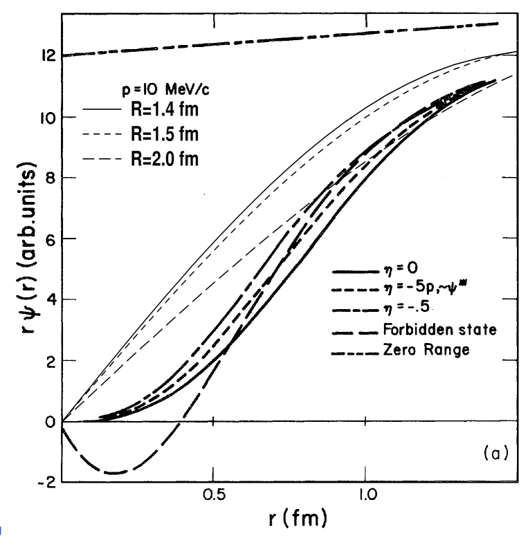
Figure 7: Our ${}^{1}S_{0}$ $nn$ scattering wave functions (thin lines) at $p=10$ MeV/c and for varying $R_{nn}$ as indicated. Here $a_{nn}=-16$ fm and $r_{0}=2.8$ fm. A comparison is made with the wave functions of the GGS model (thick lines). The latter are explained in GGS , from which reference the figure was adapted. Reprinted figure with permission from W. R. Gibbs, B. F. Gibson, and G. J. Stephenson, Jr., Phys Rev. C 11, 90 (1975). Copyright (1975) by the American Physical Society.

In Fig. 7 our $nn$ wave functions are plotted together with the wave functions used by GGS. The wave functions are quite similar in that they tend to the same asymptotic limit (the curve labeled Zero Range) for larger $r$. Thus they are very close to each other for $r\gtrsim 1.5$ fm. There are, however, a few important differences between the $nn$ wave functions in the two calculations: Firstly, the GGS wave functions have been derived using the Reid soft-core potential (RSC) (with the old larger value for the $\pi NN$ coupling constant) for the long-range part, while we used one-pion exchange only. This explains the slight difference in the size of $v(r)$ at $r=1.4$ fm. Secondly, GGS match at a fixed value of $R_{nn}=1.4$ fm, while we vary $R_{nn}$. Thirdly, our wave function uses a spherical well solution ($\sin\kappa r$) and GGS assume a polynomial of fifth order, where the magnitude and first two derivatives vanish at $r=0$ and are matched to the RSC solution at $r=R_{nn}$. The assumption of vanishing derivatives is equivalent to using a hard-core potential at short distances, while many chiral potentials have a softer behavior for small $r$ (see, e.g., Ref. Ep99 ). [The different shapes of the GGS wave functions were obtained by adding an extra term $\eta r^{3}(r-R_{nn})^{3}/pr$ to the short-range piece of their wave function.] The combined effect of all this is that our wave function has most variation around $r=1$ fm, while the GGS wave functions varies most around $\sim 0.7$ fm. As we will see later, these differences have a strong influence on the assessment of the size of the theoretical error in the extracted $a_{nn}$.

An obvious improvement of our calculation would be to use wave functions whose short-range behavior is constrained by other observables, thus reducing the uncertainty. We could also compare to wave functions of modern high-precision potentials, e.g., Refs. Wi95 ; nijmPot , or the recent N³LO chiral potentials EM03 ; Ep04 . Another extension would be to include higher partial waves.

In the actual calculations we subtract off the plane-wave $S$-wave contribution $j_{0}(pr)$ from the scattering wave function [$\tilde{v}_{0}=v_{0}-rj_{0}(pr)$] and then calculate the full plane-wave (QF or PW) contribution using $e^{i{\bf p}\cdot{\bf r}}$ without partial-wave decomposition.

III Results

III.1 Convergence

The calculated differential decay width is shown in Fig. 8 for the LO KR term only and with the NLO and NNLO one- and two-body amplitudes added in succession.

Figure 8: Time-of-flight distribution for the $\pi^{-}d\to nn\gamma$ decay rate. This and all following spectra are calculated assuming $a_{nn}=-18$ fm, $r_{0}=2.75$ fm, and $\theta_{3}=0.075$ rad, unless otherwise indicated. The plot shows the contributions from the LO KR (dotted line), NLO one-body (short-dashed line), NNLO one-body (long-dashed line), and NNLO one- and two-body (solid line) amplitudes. The two peaks are labeled QF and FSI from their dominant contributions.

The spectrum shows two separate peaks, labeled QF and FSI from the dominant contributions that give rise to them. It is clear that the LO curve is very similar to the full calculation and that the corrections of higher orders mainly affect the magnitude, but do have some impact on the shape. The evolution is most easily assessed by forming the QF to FSI peak ratio at the various orders. At LO the ratio is 2.58, at NLO 2.59, at NNLO one-body 2.60, and at full NNLO 2.71. Thus the LO, NLO, and NNLO one-body results are very close to each other, but do not contain the full dynamics that the NNLO two-body amplitudes provide. For a good quantitative result it is important to include the full NNLO amplitude—using only one-body amplitudes would give a wrong answer at this order.

III.2 Sensitivity to $a_{nn}$

In Fig. 9 the decay rate is plotted for various choices of $a_{nn}$. The curves have been rescaled to coincide at the QF peak, to facilitate comparison of the relative height of the QF and FSI peak. This is done since in the LAMPF experiment LAMPF the scattering length is extracted by fitting the shape of the spectrum, not the magnitude of the decay rate.

Figure 9: Time-of-flight distribution for the $\pi^{-}d\to nn\gamma$ decay rate. The spectrum is calculated for different choices of $a_{nn}$ as indicated. The curves for $a_{nn}=-20$ and -16 fm have been (slightly) rescaled to coincide with the QF peak of the $a_{nn}=-18$ fm curve.

Note that only the height of the FSI peak changes, the valley between the two peaks is largely unaffected by the value of $a_{nn}$.

The theoretical error in the extraction of the scattering length has several sources and they will be investigated and estimated in the following paragraphs. The error in the extracted $a_{nn}$ can be related to the error in the decay rate $\Gamma$ by

$$\frac{\Delta\Gamma}{\Gamma}=\frac{d\Gamma}{da_{nn}}\frac{a_{nn}}{\Gamma}\frac{\Delta a_{nn}}{a_{nn}},$$ (43)

where the actual calculations (Fig. 9) give that $\frac{d\Gamma}{da_{nn}}\frac{a_{nn}}{\Gamma}=1.21$ at $a_{nn}=-18$ fm. Thus

$$\frac{\Delta a_{nn}}{a_{nn}}=0.83\frac{\Delta\Gamma}{\Gamma},$$ (44)

a result we shall use repeatedly in what follows.

III.3 Theoretical error bar

We estimate the theoretical error under the assumption that the entire time-of-flight spectrum is fitted. To the best of our knowledge, previous work have only considered fitting the FSI peak, which limits the kinematics GGS ; deTeramond ; Gabioudetal . Because of the large relative momentum in the QF region, this extended analysis will have significant importance for the size of the error. We will use a nominal value of $a_{nn}=-18$ fm in our estimate of the error.

III.3.1 Neglected higher orders in the $\pi^{-}p\rightarrow\gamma n$ amplitude

The present calculation ignore pieces of the $\pi^{-}p\to\gamma n$ amplitude of $O(Q^{4})$ or higher, which is thus three orders down from the leading piece of $O(Q)$. One might think that the error would then be of the order $(\omega/\Delta)^{3}$, since the first dynamical effects not explicitly included in our Lagrangian are associated with $\Delta$-isobar excitation and so the ‘high’-energy scale is $\Delta$, the $\Delta$-nucleon mass difference, rather than $\Lambda_{\chi}$. This is supported by the results of Ref. Fearing where the fitted counter terms had unnaturally large coefficients when expressed in units of ${\rm GeV}^{-2}$. However, in Ref. Fearing the $O(Q^{3})$ one-body (single-nucleon pion photo-production) amplitude was fitted to actual data for $\omega_{0}=142$ MeV and higher (roughly 10 MeV above threshold). The error in our calculation is thus introduced only in our extrapolation of the amplitude to a subthreshold energy, denoted by $\omega^{\ast}$. Compared to the leading $O(Q)$ term, this gives a correction $(\omega_{0}^{3}-{\omega^{\ast}}^{3})/\Delta^{3}\sim 4\%$. This is a special, very beneficial feature of the pion absorption process: since the pion momentum is vanishing there is no angular dependence and the amplitudes depend only on the photon energy. This error should include the errors due to uncertainties in the LECs fitted in Fearing . A simple calculation based on the LEC fit errors and the formulas for the CGLN amplitudes gives corrections of the order 3% or smaller, which is in line with the above 4%.

Since the extrapolation photon energy is roughly the same at the QF and the FSI peak, this error should add roughly equally to both peaks, which reduces the error on the neutron time-of-flight spectrum to less than the $\sim 4\%$ estimated above, since now only the shape is fitted. The actual calculations confirm this: the spectrum using extrapolated amplitudes (see Sec. II.2.1) differs by only 1.1% in the FSI peak from the spectrum with amplitudes evaluated at threshold. The corresponding error in $a_{nn}$ is thus 0.95% or 0.17 fm for $a_{nn}=-18$ fm.

III.3.2 Boost corrections

The contribution of the boost corrections [Eqs.(20) and (21)] is of the order $\mu^{2}/2M^{2}\sim 1\%$, but the change occurs in the same direction in both peaks. Thus the relative change is much reduced ($0.14\%$ in $\Gamma_{\rm FSI}/\Gamma_{\rm QF}$, i.e., 0.11% or 0.02 fm in $a_{nn}$) and can be completely neglected for the present purposes. After rescaling, the boosted curve cannot be distinguished from the original one. We use the calculated $O(Q^{3})$ boost correction of 0.14% as a conservative estimate of the boost error introduced at higher orders. The boost correction is included in all plots.

III.3.3 Off-shellness

In calculating the one-body amplitudes we tacitly assumed that both nucleons were on-shell. This introduces an “off-shellness” error that should be estimated. It is well known that field transformations can be employed to trade dependence of the one-body amplitude on the “off-shellness” of the nucleon, $p^{0}-\frac{{\bf p}^{2}}{2M}$, for a two-body amplitude Haag ; FH . This is done as follows: using field transformations such as those employed in Refs. FS ; Fe the dependence of the $\gamma n\rightarrow\pi^{-}p$ amplitude on the nucleon energy $p^{0}$ is replaced by dependence on $\frac{{\bf p}^{2}}{2M}$ plus terms in ${\cal L}^{(3)}_{\pi N}$ and beyond. This means that the one-body amplitude for the photoproduction process now has no “off-shell ambiguity”, although we do acquire additional pieces of the two-body amplitude for the charged-pion photoproduction process. (This argument is shown graphically in the sequence of diagrams in Fig. 10.) The new contribution, depicted in Fig. 10(c), involves a $\gamma\pi\pi$ vertex from ${\cal L}_{\pi N}^{(3)}$, and so is $O(Q^{5})$. This two-body effect is thus $p^{2}/M^{2}\sim\mu^{2}/M^{2}\sim 2\%$ down from the NNLO two-body diagrams, which contribute $7.1\%$ to the rescaled decay rate (according to Fig. 8). Consequently the error in $a_{nn}$ from any potential “off-shell ambiguity” is approximately $0.02\times 0.071\times 0.83=0.12\%$ or 0.02 fm.

Figure 10: The off-shell nucleon in (a) can be taken care of by extracting a meson exchange from the deuteron wave function as in (b). The off-shell part absorbs the closest propagator and becomes the two-body diagram (c), splitting off the on-shell amplitude (d). The cross indicates an on-shell nucleon.

III.3.4 $O(Q^{4})$ two-body pieces of the amplitude

A larger effect comes from $O(Q^{4})$ two-body pieces of the $\gamma nn\rightarrow\pi^{-}d$ amplitude, such as the one depicted in Fig. 11.

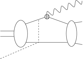
Figure 11: Typical two-body operator at $O(Q^{4})$. The sliced photo-nucleon vertex is from $\mathcal{L}_{\pi N}^{(2)}$.

A naive estimate indicates they should be $\sim p/\Lambda_{\chi}\sim\mu/\Lambda_{\chi}\sim 20$% of the $O(Q^{3})$ two-body diagrams. This estimate is supported by studies of pion photoproduction to $O(Q^{4})$ in $\chi$PT Be97 . This suggests that $O(Q^{4})$ two-body effects are roughly a 0.7% effect in $a_{nn}$.

III.3.5 Error from wave functions

Figure 12: Time-of-flight distribution for the $\pi^{-}d\to nn\gamma$ decay rate. The spectra are calculated for $a_{nn}=-18$ fm and different choices of $R_{nn}$ as indicated. The case of $R_{nn}=2.0$ fm and $a_{nn}=-18.6$ fm is also plotted.

By changing the matching points $R_{d}$ and $R_{nn}$ between 1.5 and 2.0 fm, we tested the error introduced by our ignorance of short-distance physics in the $NN$ wave functions. This change was significant for the $nn$ scattering wave functions, as shown in Fig. 12. The resulting error in $a_{nn}$ turns out to be $-0.6$ fm (3.3%) or smaller. A similar spread was obtained with wave functions calculated from “high-quality” $NN$ potentials, e.g. Nijm I and Nijm II nijmPot . We note that both these potentials have $\chi^{2}/{\rm d.o.f.}=1.03$ with respect to the 1993 Nijmegen database and identical $nn$ scattering lengths. They differ only in their treatment of the heavy mesons, indicating that our calculation is sensitive to truly short-range parts of the $NN$ interaction. Our results with the NijmI and NijmII potentials also suggest that this short-range sensitivity has a greater impact on the extracted $a_{nn}$ than does our neglect of two-pion exchange. We are confident that this uncertainty could be considerably reduced by finding other observables that constrain the wave function, in particular its short-range behavior. This will be pursued in future work. Note that the change in $R_{nn}$ not only changes the height of the FSI peak, but also the valley region. This feature could potentially be used in a fit procedure to distinguish the $R_{nn}$ dependence from a change in $a_{nn}$.

Indeed, if one focuses only on the FSI peak then the variation in the spectrum due to the use of different wave functions is significantly smaller than the one discussed in the previous paragraph. If we adjust both calculations to agree in the valley region we find that the FSI peak height only differs by 0.6%. (See Fig. 13.) This corresponds to an uncertainty in $a_{nn}$ of $\pm 0.1$ fm.

Figure 13: Time-of-flight distribution for the $\pi^{-}d\to nn\gamma$ decay rate in the region of the FSI peak. The spectra are calculated for $a_{nn}=-18$ fm and different choices of $R_{nn}$ as indicated.

Meanwhile, effects due to the bound-state wave function chosen are also small. Changing the deuteron wave function by varying $R_{d}$ from 2.0 fm to 1.5 fm would alter the extracted $a_{nn}$ by 0.55% or 0.10 fm. Using the Bonn B deuteron wave function instead of the EFT-motivated wave function yields a $\Delta a_{nn}$ of 0.56% or 0.10 fm.

III.3.6 Higher partial waves

The error from neglecting higher partial waves in the rescattering wave function can be estimated in the following way. The higher partial waves are only substantial for large relative energies and are thus negligible in the FSI peak region. In the QF peak, the relative $nn$ momentum is roughly 80 MeV/$c$, which means that the $S$-wave phase shift is $\delta_{0}\lesssim 60^{\circ}$, while the $P$-wave phase shifts are typically $\delta_{1}\lesssim 5^{\circ}$. The $P$- to $S$-wave amplitude ratio can then be estimated as $A_{1}/A_{0}\sim\sin\delta_{1}/\sin\delta_{0}=0.10$.

Figure 14: The decay rate separated into spin-0 and spin-1 contributions. The subtracted FSI ${}^{1}S_{0}$ partial wave is also distinguished.

From Fig. 14 the $S$-wave FSI amplitude at the QF peak is $A_{0}=\sqrt{0.030}=0.17$ and thus the $P$-wave FSI amplitude is $A_{1}\sim 0.10A_{0}=0.017$. However, since the $P$-waves are spin-1 and the $S$-waves spin-0 and the two do not interfere, the influence of the $P$-wave should be related to the QF spin-1 amplitude, which is $B_{1}=\sqrt{0.295}=0.543$. The error in the calculated QF peak is then $2|A_{1}||B_{1}||\cos\theta|$, where $\theta$ is the unknown phase angle between $A_{1}$ and $B_{1}$. Using the maximal possible error (setting $\cos\theta=1$) seems overly pessimistic, so we instead choose the average $\langle|\cos\theta|\rangle=2/\pi$. The relative error at the QF peak is then $\frac{4}{\pi}|A_{1}||B_{1}|/\Gamma_{\rm QF}\sim 2.9\%$, yielding an error in the extracted scattering length of 2.4% or 0.43 fm. This should be regarded as a conservative estimate of the error of neglecting $P$-waves for two reasons. Firstly, the $P$-waves could interfere destructively with each other. And secondly, we implicitly assume that the radial integral for $P$-waves is of the same magnitude as for $S$-waves, whereas it is probably smaller. Most importantly, it is possible to actually calculate and include the $P$-waves. This error can thus easily be pushed to higher partial waves and so made substantially smaller. This will be done in future work.

Note that this $P$-wave error is much larger than the one estimated by GGS GGS . The reason is that the $P$-waves only contribute at large relative energy, i.e., under the QF peak, where they can interfere with the QF amplitudes, thus changing the QF to FSI peak ratio and the extracted $a_{nn}$. The GGS error estimate assumes that the $nn$ opening angle is smaller than $30^{\circ}$, which restricts the kinematics to the FSI peak region only and thus does not apply to the entire range of neutron energies used in the LAMPF extraction. Also in the work of de Téramond et al. deTeramond as used by the PSI group Gabioudetal , only the FSI peak region is fitted, which gives a small $P$-wave contribution. Thus, as far as we can ascertain, our analysis is the first that estimates the interference of the FSI $P$-waves with the spin-1 QF amplitude.

If this effect was not included in the analysis of the data in Ref. LAMPF then the $\Delta a_{nn}$ of approximately 0.43 fm we have found here should be included in the theoretical uncertainty quoted in that work. However, correspondence with one of the authors of Ref. LAMPF suggests that FSI in $NN$ $P$-waves was included in the version of the GGS model used for the $a_{nn}$ extraction there Ben . This source of uncertainty would then not be present in Ref. LAMPF ’s value for $a_{nn}$.

III.3.7 Sensitivity to $r_{0}$

An estimate of a change in $r_{0}$ due to CSB can be obtained by assuming that the relative change in $r_{0}$ is similar to the relative change in $a_{NN}$. Thus $\frac{\Delta r_{0}}{r_{0}}\approx\frac{\Delta a}{a}$ so that $\Delta r_{0}=\frac{r_{0}}{a}\Delta a=\frac{2.75}{18}1.5=0.23$ fm. The sensitivity to the effective-range parameter $r_{0}$ was tested by varying it away from its nominal value $2.75$ fm, using a conservative spread of $\pm 0.25$ fm. This changes the FSI peak by $1.4\%$ (after rescaling to the QF peak) and thus indicates a change in the extracted $a_{nn}$ of 1.2% or 0.21 fm. On the other hand, the error suggested by analysis of different experimental determinations of $r_{0}$ is $\pm 0.11$ fm Slaus . If $r_{0}$ is instead varied over this narrower range the resultant $\Delta a_{nn}$ is only 0.5% or 0.09 fm. We will use the latter, smaller, error in our error budget.

III.4 Error budget

The errors are summarized in Table 1.

Table 1: Error budget for the extraction of $a_{nn}$ from the $\pi^{-}d\to nn\gamma$ reaction as it was performed in Ref. LAMPF . The calculation of the absolute errors assumes a scattering length of -18 fm. The total error is summed in quadrature.

Source	Relative error (%)	Absolute error (fm)
Off-shell	$0.07$	$0.01$
Boost	$<0.11$	$<0.02$
Subthreshold	$0.95$	$0.17$
$O(Q^{4})$ 2B	$0.7$	$0.12$
$r_{0}$	$0.5$	$0.09$
Dep. on $R_{d}$	$0.55$	$0.10$
$p$-wave in FSI	$<2.4$	$<0.43$
Dep. on $R_{nn}$	$<3.3$	$<0.60$
total	$<4.3$	$<0.78$

The first four errors are due to uncertainties in the amplitudes, while the last four are due to the wave functions . We consider the total error of $<4.3\%$ to be a very conservative estimate.

Note that if $a_{nn}$ is extracted only from data in the FSI region then the last two errors drop to 0.2% and 0.5% respectively, while a number of the other errors listed in Table 1 are also reduced. We find that an extraction performed using only data from this section of the neutron time-of-flight spectrum would have a theoretical uncertainty of $\pm 0.2$ fm. This confirms the conclusion of GGS from thirty years ago. The significantly reduced theoretical uncertainty comes at a price though: one must sacrifice the large number of counts acquired under the QF peak. We have argued above that the last two errors quoted in Table 1 can be decreased by additional theoretical work on radiative pion-capture on deuterium, and therefore we hold out hope that in future a $\chi$EFT extraction of $a_{nn}$ which has an accuracy of $\pm 0.3$ fm (or better) and uses the full neutron spectrum obtained in Ref. LAMPF can be performed.

One reason for this optimism is the convergence of the chiral expansion for this reaction, which can be made more explicit by computing the QF to FSI peak ratio for the different orders. From Fig. 8 we obtain

$$\frac{\Gamma_{\rm QF}}{\Gamma_{\rm FSI}}=(2.580+0.014+0.112\pm 0.039)(1\pm 0.05),$$ (45)

where the first parenthesis contains (in order) the contribution of the LO, NLO, NNLO, and the error in the chiral expansion. The second parenthesis shows the error due to effects in the wave functions. Note that modifying the wave functions by including two-pion exchanges, $P$-waves, or different short-distance dynamics would already change the LO calculation, which is why we choose to write this error as an overall factor. The smallness of the NLO and NNLO one-body terms can perhaps be an effect of the particular kinematics of the present problem, especially that the pion momentum is vanishing. On the other hand, the comparatively large NNLO two-body contribution is most likely a result of a combination of two effects: Firstly, the two-body currents allow for momentum sharing between the nucleons, which would be of importance in the QF region. Secondly, in the leading two-body diagram [Fig. 5(a)], the coulombic propagator was power-counted as $1/\mu^{2}$. However, because of the small deuteron binding energy, the typical momentum is instead of the order $\gamma=\sqrt{MB}=45.7$ MeV pid . Since $\gamma\ll\mu$ this further enhances this diagram.

IV Conclusions

In this paper we have calculated the $\pi^{-}d\to nn\gamma$ reaction, using $\chi$PT pion-photon amplitudes and EFT-inspired wave functions. The errors in the extracted scattering length from the operators are of the order 1%. These errors include effects that were not considered by Gibbs, Gibson, and Stephenson (GGS) GGS , e.g., errors from extrapolating the single-nucleon amplitudes sub-threshold, the boost of the $\gamma n\to\pi^{-}p$ amplitude from the $\gamma n$ rest frame to c.m., the effects of off-shell nucleons, and more complicated two-body mechanisms. A key improvement is that we have included the full two-body amplitude at third chiral order and have found that on the scale of the other errors it has a substantial influence on the extraction of the scattering length.

Nevertheless, if $a_{nn}$ is extracted from the FSI region alone our analysis within $\chi$EFT confirms GGS’s result for the theoretical uncertainties, putting them at $\pm 0.2$ fm. On the other hand, if—as was done in the most recent $a_{nn}$ extraction LAMPF —the entire shape of the neutron spectrum, including both the QF and FSI peaks, is used for the extraction, then the uncertainty in the scattering wave function at small distances and the neglect of higher partial waves is a potentially large source of errors, maybe as large as 4.3%. This might seem like a large uncertainty, since it is almost three times larger than the 1.5% estimated by GGS. But, as was argued in Sec. III.3.5, some of the assumptions behind their error estimate do not seem to apply for the entire kinematic range spanned by the data from the LAMPF experiment. This tempts us to suggest that the error estimate given in Ref. LAMPF is optimistic and should be increased.

We plan to improve our model in the near future by constraining the short-distance part of the $nn$ wave function using other observables and by incorporating higher partial waves. We will report these results in a future publication. We also plan to fold our model with the neutron detector acceptance and the experimental geometry in order to extract the $nn$ scattering length from the data of Ref. LAMPF .

Overall we conclude that the $\pi^{-}d\to nn\gamma$ reaction has some very desirable features that makes it extremely suitable for the extraction of the neutron-neutron scattering length. The vanishing pion momentum obviously favors a $\chi$PT calculation and also reduces the number of contributing terms dramatically, leading to the dominance of the Kroll-Ruderman term. The fact that the extraction is done by fitting the shape of time-of-flight spectra rather than an absolute decay rate reduces many errors further still.

The reaction $\gamma d\to nn\pi^{+}$ could be used as an alternative and complementary way to extract the neutron-neutron scattering length. This reaction has been considered before, see the review Laget and later papers, e.g., Ulla . A chiral calculation should be feasible for this reaction, and could benefit from the work of the present paper. With a threshold photon laboratory energy of $149$ MeV it should be accessible at existing experimental facilities, e.g., HI$\gamma$S@TUNL after the planned upgrade and MAX-lab in Lund, Sweden. After the submission of the manuscript, a calculation of $\gamma d\to nn\pi^{+}$ using chiral perturbation theory along lines similar to ours has become available Lensky:2005hb .

- (1) G. A. Miller, B. M. K. Nefkens, and I. Šlaus, Phys. Rep. 194, 1 (1990).
- (2) E. J. Stephenson et al., Phys. Rev. Lett. 91, 142302 (2003).
- (3) A. K. Opper et al., Phys. Rev. Lett. 91, 212302 (2003).
- (4) W. I. Furman et al., J. Phys. G: Nucl. Part. Phys. 28, 2627 (2002).
- (5) V. Huhn et al., Phys. Rev. Lett. 85, 1190 (2000).
- (6) D. E. González Trotter et al., Phys. Rev. Lett. 83, 3788 (1999).
- (7) I. Šlaus, Y. Akaishi, and H. Tanaka, Phys. Rep. 173, 257 (1989).
- (8) R. B. Wiringa, V. G. J. Stoks, and R. Schiavilla, Phys. Rev. C 51, 38 (1995).
- (9) S. C. Pieper and R. B. Wiringa, Annu. Rev. Nucl. Part. Sci. 51, 53 (2001).
- (10) C. R. Howell et al., Phys. Lett. B 444, 252 (1998).
- (11) W. R. Gibbs, B. F. Gibson, and G. J. Stephenson, Jr., Phys Rev. C 11, 90 (1975); 12 2130(E) (1975); 16, 322 (1977); 16, 327 (1977); 17, 856(E) (1978).
- (12) B. Gabioud et al., Phys. Rev. Lett. 42, 1508 (1979); Phys. Lett. 103B, 9 (1981); Nucl. Phys. A420, 496 (1984); O. Schori, B. Gabioud, C. Joseph, J. P. Perroud, D. Rüegger, M. T. Tran, P. Truöl, E. Winkelmann, and W. Dahme, Phys. Rev. C 35, 2252 (1987).
- (13) G. F. de Téramond, Phys. Rev. C 16, 1976 (1977); G. F. de Téramond, J. Páez, and C. W. Soto Vargas, ibid. 21, 2542 (1980); G. F. de Téramond and B. Gabioud, ibid. 36, 691 (1987).
- (14) T. Becher and H. Leutwyler, Eur. Phys. J. C 9, 643 (1999).
- (15) T. Fuchs, J. Gegelia, G. Japaridze and S. Scherer, Phys. Rev. D 68, 056005 (2003).
- (16) V. Bernard, N. Kaiser, and U.-G. Meißner, Int. J. Mod. Phys. E 4, 193 (1995).
- (17) G. Ecker and M. Mojžiš, Phys. Lett. B 365, 312 (1996).
- (18) H. W. Fearing, T. R. Hemmert, R. Lewis, and C. Unkmeir, Phys. Rev. C 62, 054006 (2000).
- (19) G. F. Chew, M. L. Goldberger, F. E. Low, and Y. Nambu, Phys. Rev. 106, 1345 (1957).
- (20) S. R. Beane, C. Y. Lee, and U. van Kolck, Phys. Rev. C 52, 2914 (1995).
- (21) V. Baru, C. Hanhart, A. E. Kudryavtsev and U. G. Meißner, Phys. Lett. B 589, 118 (2004).
- (22) S. R. Beane, V. Bernard, T.-S. H. Lee, U.-G. Meißner, and U. van Kolck, Nucl. Phys. A618, 381 (1997).
- (23) V. G. J. Stoks, R. A. M. Klomp, M. C. M. Rentmeester, and J. J. de Swart, Phys. Rev. C 48, 792 (1993); U. van Kolck, M. C. M. Rentmeester, J. L. Friar, T. Goldman, and J. J. de Swart, Phys. Rev. Lett. 80, 4386 (1998).
- (24) S. Weinberg, Phys. Lett., B251, 288 (1990); Nucl. Phys. B363, 3 (1991).
- (25) C. Ordonéz, L. Ray, and U. van Kolck, Phys. Rev. C 53, 2086 (1996).
- (26) N. Kaiser, R. Brockmann, and W. Weise, Nucl. Phys. A625, 758 (1997).
- (27) E. Epelbaum, W. Glöckle, and U.-G. Meißner, Nucl. Phys. A671, 295 (1999).
- (28) M. C. M. Rentmeester, R. G. E. Timmermans, J. L. Friar, and J. J. de Swart, Phys. Rev. Lett. 82, 4992 (1999).
- (29) J. J. de Swart, C. P. F. Terheggen, and V. G. J. Stoks, nucl-th/9509032.
- (30) D. R. Phillips and T. D. Cohen, Nucl. Phys. A668, 45 (2000).
- (31) V. Stoks, R. Timmermans, and J. J. de Swart, Phys. Rev. C 47, 512 (1993).
- (32) G. P. Lepage, arXiv:nucl-th/9706029.
- (33) V. G. J. Stoks, R. A. M. Klomp, C. P. F. Terheggen, and J. J. de Swart, Phys. Rev. C 49, 2950 (1994).
- (34) S. R. Beane, P. F. Bedaque, M. J. Savage, and U. van Kolck, Nucl. Phys. A700, 377 (2002).
- (35) D. R. Entem and R. Machleidt, Phys. Rev. C 68, 041001(R) (2003).
- (36) E. Epelbaum, W. Glöckle, and U.-G. Meißner, arXiv:nucl-th/0405048.
- (37) R. Haag, Phys. Rev. 112, 669 (1958).
- (38) R. J. Furnstahl and H. W. Hammer, Phys. Lett. B 531, 203 (2002).
- (39) S. Scherer and H. W. Fearing, Phys. Rev. D 52, 6445 (1995).
- (40) S. Scherer and H. W. Fearing, Phys. Rev. C 51, 359 (1995); H. W. Fearing, Phys. Rev. Lett. 81, 758 (1998); H. W. Fearing and S. Scherer, Phys. Rev. C 62, 034003 (2000).
- (41) B. F. Gibson, private communication (2005).
- (42) S. R. Beane, V. Bernard, E. Epelbaum, U.-G. Meißner, and D. R. Phillips, Nucl. Phys. A720, 399 (2003).
- (43) J. M. Laget, Phys. Rep. 69, 1 (1981).
- (44) G. Fäldt and U. Tengblad, Physica Scripta 34, 742 (1986); U. Tengblad, Ph.D. Thesis, Uppsala University, (1987).
- (45) V. Lensky, V. Baru, J. Haidenbauer, C. Hanhart, A. E. Kudryavtsev, and U.-G. Meißner, arXiv:nucl-th/0505039.