Solar Hydrogen Burning and Neutrinos

Abstract

We summarize the current status of laboratory measurements of nuclear cross sections of the pp chain and CN cycle. We discuss the connections between such measurements, predictions of solar neutrino fluxes, and the conclusion that solar neutrinos oscillate before reaching earth.

1 Introduction

The probable role of thermonuclear reactions in generating energy within the solar interior was recognized as early as the 1920s by astrophysicists such as Eddington [1]. This deduction came about by default, rather than by any direct laboratory observation of the reactions. Once the earth’s age was established to be at least a few billion years old (see Burchfield [2] for an interesting history of the development of this idea), it became apparent that gravitational and chemical energy sources could not sustain solar evolution, given the known mass, radius, and luminosity of the sun. In contrast, newly discovered nuclear reactions and decays could readily supply the required energy over the requisite time. A key step was taken by Gamow [3], who recognized that tunnelling under the Coulomb barrier could enable nuclear reactions to occur at the low energies typical of the solar interior, where kT $\sim$ a few keV (e.g., Atkinson $\&$ Houtermans [4]). This idea and subsequent investigations led to descriptions of possible reaction chains for stellar energy generation. By the end of the 1930s Weizsacker [5, 6], Bethe $\&$ Critchfield [7], and Bethe [8] had described the essential features of the carbon-nitrogen cycle and the proton–proton chain, the processes by which the sun and similar stars convert hydrogen to helium.

The neutrino has a similar vintage, and was connected early on to stellar reactions. In December 1930 Wolfgang Pauli proposed that the emission of an unobserved spin–1/2 neutral particle – the electron neutrino ($\nu_{e}$) – might explain the apparent lack of energy conservation in nuclear beta decay

$$(A,Z)\to(A,Z-1)+e^{+}+\nu_{e}$$

Enrico Fermi was present at a number of Pauli’s presentations and discussed the neutrino with him on these occasions. In 1934, following closely Chadwick’s discovery of the neutron, Fermi proposed a theory of beta decay based on Dirac’s description of electromagnetic interactions, but with weak currents interacting at a point, rather than at long distance through the electromagnetic field. He described beta decay as a proton decaying to a neutron, a phenomenon energetically possible because of nuclear binding energies, with the emission of a positron and neutrino. Apart from the absence of parity violation, which would not be discovered until 1957, Fermi’s description is a correct low-energy approximation to our current standard model of weak interactions.

Thus, as nuclear astrophysicists unravelled the stellar processes for hydrogen burning, stars were recognized to be copious sources of neutrinos

$$4p\to{}^{4}\rm{He}+2e^{+}+2\nu_{e}$$

This observation led Ray Davis to construct the chlorine experiment to measure the flux of solar neutrinos. The resulting solar neutrino puzzle was ultimately traced to new physics (neutrino oscillations) requiring the mixing of massive neutrinos, a phenomenon beyond the standard electroweak model. This discovery depended critically on the reliability of solar model neutrino flux predictions, and thus on the quality of our understanding of the nuclear reaction rates governing the pp and CN cycles.

The goal of this paper is to summarize our understanding of solar hydrogen burning, with special emphasis on the connections between laboratory astrophysics—measurement of nuclear cross sections at or near energies characteristic of the solar core—and the predictions of solar neutrino fluxes.

2 Hydrogen Burning

Observations of stars reveal a wide variety of stellar conditions, with luminosities relative to solar spanning a range $L\sim$ 10^-4 to 10⁶ $L_{\odot}$ and surface temperatures $T_{s}\sim$2000–50000 K. The simplest relation one could propose between luminosity $L$ and $T_{s}$ is that for a blackbody

$$L\,=\,4\pi R^{2}\sigma\,T_{s}^{4}\Rightarrow L/L_{\odot}\,=\,(R/R_{\odot})^{2}\,(T_{s}/T_{\odot})^{4}$$ (1)

which suggests that stars of a similar structure might lie along a one–parameter path (corresponding to $R/R_{\odot}$ above) in the luminosity (or magnitude) vs. temperature (or color) plane. In fact, there is a dominant path in the Hertzsprung–Russell color–magnitude diagram along which roughly 80$\%$ of the stars reside. This is the main sequence, those stars supporting themselves by hydrogen burning through the pp chain or CN cycles.

As one such star, the sun is an important test of our theory of main sequence stellar evolution: its properties – age, mass, surface composition, luminosity, and helioseismology – are by far the most accurately known among the stars. The standard solar model (SSM) traces the evolution of the sun over the past 4.6 billion years of main sequence burning, thereby predicting the present–day temperature and composition profiles, the relative strengths of competing nuclear reaction chains, and the neutrino fluxes resulting from those chains. Standard solar models share four basic assumptions:

• The sun evolves in hydrostatic equilibrium, maintaining a local balance between the gravitational force and the pressure gradient. To describe this condition in detail, one must specify the equation of state as a function of temperature, density, and composition.

• Energy is transported by radiation and convection. While the solar envelope is convective, radiative transport dominates in the core region where thermonuclear reactions take place. The opacity depends sensitively on the solar composition, particularly the abundances of heavier elements.

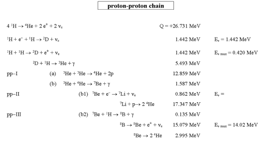
Figure 1: The pp–chain, showing the three terminations: ppI, ppII, and ppIII.

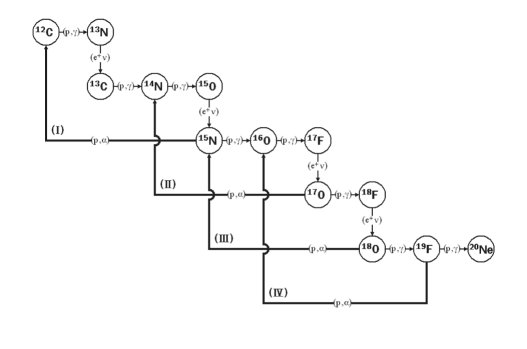
Figure 2: The primary CN–cycle, together with three subsidiary cycles which can bypass the ¹⁵N(p,$\alpha)^{12}$C termination to extend this processing as far as ²⁰Ne.

• Thermonuclear reaction chains generate solar energy. The standard model predicts that over 98$\%$ of this energy is produced from the pp chain conversion of four protons into ⁴He (see Fig. 1), with proton burning through the CN cycle contributing the remaining 2$\%$ (Fig. 2). The Sun is a large but slow reactor: the core temperature, $T_{c}\sim$1.5 $\times$ 10⁷ K, results in typical center-of-mass energies for reacting particles of $\sim$ 10 keV, much less than the Coulomb barriers inhibiting charged particle nuclear reactions. Thus reaction cross sections are small: in most cases, laboratory measurements are only possible at higher energies, so that cross section data must be extrapolated to the solar energies of interest.

• The model is constrained to produce today’s solar radius, mass, and luminosity. An important assumption of the standard model is that the Sun was highly convective, and therefore uniform in composition, when it first entered the main sequence. It is furthermore assumed that the surface abundances of metals (nuclei with A $>$ 5) were undisturbed by the subsequent evolution, and thus provide a record of the initial solar metalicity. The remaining parameter is the ⁴He/H ratio, which is adjusted until the model reproduces the present solar luminosity after 4.6 billion years of evolution. The resulting ⁴He/H mass fraction ratio is typically 0.27 $\pm$ 0.01, which can be compared to the big–bang value of 0.23 $\pm$ 0.01. Note that the Sun was formed from previously processed material.

The model that emerges is an evolving Sun. As the core’s chemical composition changes, the opacity and core temperature rise, producing a 44$\%$ luminosity increase since its arrival on the main sequence. The temperature rise governs the competition between the three cycles of the pp chain: the ppI cycle dominates below about 1.6 $\times$ 10⁷ K; the ppII cycle between (1.7–2.3) $\times$ 10⁷ K; and the ppIII above 2.4 $\times$ 10⁷ K. The central core temperature of today is about 1.55 $\times$ 10⁷ K.

This competition between the cycles determines the pattern of neutrino fluxes. One consequence of the thermal evolution of our sun is the relatively recent appearance of a significant ⁸B neutrino flux, the species that dominated the Davis experiment. As this flux is produced in the ppIII cycle, it is a very sensitive function of the solar core. The SSM predicts an exponential increase in this flux with a doubling period of about 0.9 billion years.

A final aspect of SSM evolution is the formation of composition gradients on nuclear burning timescales. Clearly there is a gradual enrichment of the solar core in ⁴He, the ashes of the pp–chain. Another element, ³He, is produced and then consumed in the pp chain, eventually reaching some equilibrium abundance. The time–scale for equilibrium to be established as well as the eventual equilibrium abundance are both sharply decreasing functions of temperature, and thus increasing functions of the distance from the center of the core. Thus a steep ³He density gradient is established over time.

The SSM has had some notable successes. From helioseismology the sound speed profile $c(r)$ has been very accurately determined for the outer 90$\%$ of the Sun, and is in good agreement with the SSM. (However, this conclusion depends in part on inputs to the SSM: recent calculations employing one set of revised opacities do show some significant discrepancies, as we will discuss later.) Helioseismology probes important predictions of the SSM, such as the depth of the convective zone. The SSM is not a complete model in that it does not attempt to describe from first principles aspects such as convection that extend beyond 1D descriptions. For this reason certain features of solar structure, such as the depletion of surface Li by two orders of magnitude, are not reproduced. Li destruction is often attributed to convective processes that operated at some epoch in our sun’s history, dredging Li to a depth where burning takes place.

3 Reaction Rate Formalism

3.1 Nuclear rates and S-factors

Perhaps the key step that allowed quantitative modelling of the sun and other main–sequence stars was the description of the relevant nuclear reaction chains. This required both the development of a theory for sub–barrier fusion reactions and careful laboratory measurements to constraint the rates of these reactions at stellar temperatures.

At the temperatures and densities in the solar interior (e.g., $T_{c}\sim$ 15 $\times$ 10⁶ K and $\rho_{c}\sim$ 153 g/cm³ [9]), interacting nuclei reach a Maxwellian equilibrium distribution in a time that is infinitesimal compared to nuclear reaction time scales. Therefore, the reaction rate between two nuclei can written as (e.g., Burbidge et al., [10]; Clayton [11]; Rolfs $\&$ Rodney [12]):

$$r_{12}\,=\,\frac{n_{1}\,n_{2}}{1+\delta_{12}}\,\langle{\sigma v}\rangle_{12}.$$ (2)

Here the Kronecker delta prevents double counting in the case of identical particles, $n_{1}$ and $n_{2}$ are the number densities of nuclei of type 1 and type 2 (with atomic number $Z_{1}$ and $Z_{2}$, and atomic mass $A_{1}$ and $A_{2})$, and $\left\langle{\sigma v}\right\rangle_{12}$ denotes the product of the reaction cross–section and the relative velocity $v$ of the interacting nuclei, averaged over the collisions in the stellar gas,

$$\langle\sigma v\rangle_{12}\,=\,\int_{0}^{\infty}\,[\,\sigma\,(v)\,\cdot\,v]\,\Phi\,(v)\,\mbox{d}v.$$ (3)

Under solar conditions nuclear velocities are very well approximated by a Maxwell–Boltzmann distribution. It follows that the relative velocity distribution is also a Maxwell–Boltzmann, governed by the reduced mass $\mu$ of the colliding nuclei,

$$\Phi\,(v)\mbox{ d}v=(\frac{\mu}{2\pi kT})^{3/2}\mbox{ exp}(-\frac{\mu v^{2}}{2kT})4\pi v^{2}\mbox{ d}v.$$ (4)

Therefore,

$$\langle{\sigma v}\rangle_{12}\,=\,[\,\frac{8}{\pi\mu(kT)^{3}}\,]^{1/2}\,\int_{0}^{\infty}\,E\,\sigma\,(E)\mbox{ exp}\,(\,-\frac{E}{kT}\,)\mbox{ d}E,$$ (5)

where $E$ is the relative kinetic energy in the center–of–mass system. In order to evaluate $\left\langle{\sigma v}\right\rangle$ the energy dependence of the reaction cross-section must be determined. (In Fowler et al. [13] and more recently in Angulo et al. [14], the appropriate expressions for $\left\langle{\sigma v}\right\rangle$ are tabulated for a variety of specific reactions, including both non-resonant and resonant neutron-induced and charged-particle-induced reactions.)

Almost all of the nuclear reactions relevant to solar energy generation are nonresonant and charged–particle induced. For such reactions, as the energy dependence at low energies is dominated by the Coulomb barrier, cross sections are typically expressed in terms of the S–factor,

$$\sigma\left(E\right)\;=\;\frac{S\left(E\right)}{E}\;\;\mathrm{exp}\left({-2\pi\eta}\right),$$ (6)

where the 1/$E$ term comes from the $\lambda^{2}$ geometrical factor, exp$\left({-2\pi\eta}\right)$ is the usual Gamow barrier penetration term with $\eta$ = $Z_{1}Z_{2}$ $\alpha$/$v$, $v$ is the relative velocity, and $\alpha\sim$ 1/137 is the fine structure constant. (We take $\hbar$ = c = 1.) That is, the sharp energy dependence associated with s–wave interactions of point nuclei has been removed from $\sigma(E)$, leaving a quantity $S(E)$ that contains the nontrivial nuclear physics, yet is simpler to model over an energy range spanning both solar reactions and terrestrial laboratory measurements. For nonresonant reactions $S(E)$ will be a slowly varying function of $E$.

One must take into account differences in the atomic environments to correctly relate laboratory measurements of $\sigma$$(E)$ and $S(E)$ to the corresponding quantities in the solar interior. As light nuclei in the solar core are almost completely ionized, the solar electron screening correction $f_{0}$ can be treated in a weak–screening approximation [15]. The correction depends on the ratio of the Coulomb potential at the Debye radius $R_{D}$ to the temperature,

$$f_{0}=\;\mathrm{exp}\left({Z_{1}\,Z_{2}\;\alpha\over R_{D}kT}\right)=\;\mathrm{exp}\left({0.188\,Z_{1}\,Z_{2}\;\zeta\;\rho_{0}^{1/2}\;T_{6}^{-3/2}}\right),$$ (7)

where $\zeta R_{D}=\left({kT\over 4\pi\alpha\rho}\right)^{1/2}$, $\rho$ is the number density of nucleons, $\rho_{0}$ is a dimensionless density measured in g/cm³, $\zeta$ = [$\sum\limits_{i}$ ($X_{i}\,\frac{Z_{i}^{2}}{A_{i}}$ + $X_{i}$; $\frac{Z_{i}}{A_{i}}$) ] ^1/2, $X_{i}$ is the mass fraction of nuclei of type $i$, and $T_{6}$ is the dimensionless temperature in units of 10⁶ K. Note that the screening factor enhances solar cross sections.

Substituting (4) into (1) yields

$$\left\langle{\sigma v}\right\rangle_{12}=\;\left[{\frac{8}{\pi\mu(kT)^{3}}}\right]^{1/2}f_{0}\;\int\limits_{0}^{\infty}{\;S\left(E\right)}\;\exp\left({-2\pi\eta}\right)\;\exp\left({-E/kT}\right)\;\mathrm{d}E.$$ (8)

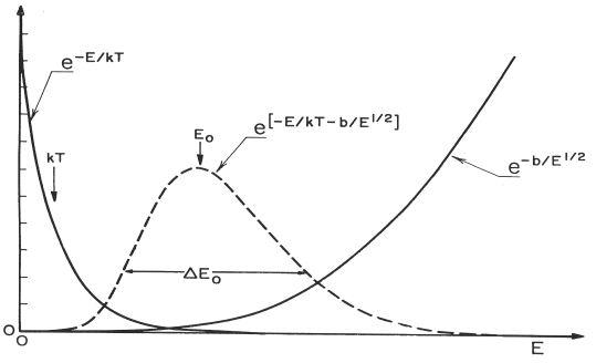
Figure 3: The energy dependence of the integrand in Eq. (6), defining the parameters of the Gamow peak.

The energy dependence of this integrand is shown schematically in Fig. 3. In order to evaluate this integral we expand $S(E)$ in a Taylor series,

$$S(E)=S(0)+ES^{\prime}(0)+\frac{1}{2}E^{2}S^{\prime\prime}(0)+.......$$ (9)

Substituting this into (6) yields (Bahcall [16]),

$$\left\langle{\sigma v}\right\rangle_{12}=\;\left({\frac{2}{\mu kT}}\right)^{1/2}\left({\Delta\,E_{0}/kT}\right)\left({f_{0}\,S_{eff}}\right)\;\exp\left({-3E_{0}/kT}\right)\hskip 42.67912pt$$ (10)

$$=1.301\times 10^{-14}\mathrm{cm}^{3}/\mathrm{s}\left({\frac{Z_{1}\,Z_{2}}{A}}\right)^{1/3}f_{0}\;{S_{eff}\over MeV-b}\;T_{9}^{-2/3}\exp\left({-3E_{0}/kT}\right)$$

where

$$E_{0}/kT=(\pi Z_{1}Z_{2}\alpha/\sqrt{2})^{2/3}(\mu c^{2}/kT)^{1/3},$$

$$\Delta E_{0}/kT=4[E_{0}/3kT]^{1/2},~{}~{}~{}~{}~{}~{}~{}A={A_{1}A_{2}\over A_{1}+A_{2}},$$

and

$$S_{eff}=S(0)[1+\frac{5kT}{36E_{0}}]+S^{\prime}(0)E_{0}[1+\frac{35kT}{36E_{0}}]+\frac{1}{2}S^{{}^{\prime\prime}}(0)E_{0}^{2}[1+\frac{89kT}{36E_{0}}].$$

$E_{0}$ corresponds to the maximum of the integrand, the Gamow peak, and is thus the most probable energy of reacting nuclei (see Fig. 3). $\Delta E_{0}$ corresponds to the full width of the integrand at 1/$e$ of its maximum value. (For example, for a typical solar core temperature of $T_{6}$ = 16, $E_{0}$ = 23.4 keV and $\Delta E_{0}$= 13.1 keV for the ³He($\alpha$,$\gamma)^{7}$Be reaction in the proton-proton chain.)

Numerous laboratory measurements have been carried out to determine $S$(0), $S^{\prime}$(0), and $S^{\prime\prime}$(0) for the various nuclear reactions contributing to the proton–proton chain and the CN cycle. At the present time it is not technically feasible to measure the cross sections for most of these reactions in the region of $E_{0}$, as the cross sections are severely suppressed by the Coulomb barrier. (Clearly, as the basic timescale is the solar age, the sun is a very slow reactor operating at a temperature where many reactions are highly suppressed.) Therefore $S_{eff}$ often must be determined from extrapolations from laboratory measurements at higher energies, typically $E\mathrel{\hbox to0.0pt{\lower 4.0pt\hbox{\hskip 1.0pt$\sim$}\hss}\raise 1.0pt\hbox{$>$}}$ 100 to 200 keV.

So far, the one significant reaction for which it has been possible to measure the cross section down to $E_{0}$ is the ³He(³He,2p)⁴He reaction – see Section 4.3, below. At the sun’s center, $E_{0}\sim$ 22 keV for this reaction. The measured cross section is $\sigma(E_{0})\sim$1.5 pb. This can be compared with the cross sections for the (p,$\gamma)$ and ($\alpha$,$\gamma)$ capture reactions that contribute in the pp chain or CN cycle, e.g.,

³He($\alpha$,$\gamma)^{7}$Be $\rightarrow E_{0}$ $\sim$ 23 keV $\rightarrow\sigma(E_{0})$ $\sim$ 3 $\times$ 10^-5 pb

⁷Be(p,$\gamma)^{8}$B $\rightarrow E_{0}$ $\sim$ 18.4 keV $\rightarrow\sigma$($E_{0})\sim$ 1.5 $\times$ 10^-3 pb

¹⁴N(p,$\gamma)^{15}$O $\rightarrow E_{0}$ $\sim$ 27.2 keV $\rightarrow\sigma(E_{0})\sim$ 2.2 $\times$ 10^-7 pb

Direct measurements of these much smaller capture cross sections at $E_{0}$ are not anticipated without orders of magnitude improvements in sensitivity.

For completeness we can also evaluate Eq. (5) for the case of a reaction dominated by a narrow, isolated resonance,

$$\int\limits_{0}^{\infty}{E\,\sigma\left(E\right)}\,\exp\left({-E/kT}\right)\,\mathrm{d}E=E_{res}\exp\left({-E_{res}/kT}\right)\int\limits_{0}^{\infty}\sigma\left(E\right)\,\mathrm{d}E$$ (11)

Assuming a Breit–Wigner line shape $\sigma\left(E\right)=\sigma_{BW}\left(E\right)=\pi\mathchar 22\relax\mkern-10.0mu\lambda^{2}\omega\,\,\frac{\Gamma_{1}\Gamma_{2}}{\left({E_{res}-E}\right)^{2}+{\Gamma^{2}}\mathord{\left/{\vphantom{{\Gamma^{2}}4}}\right.\kern-1.2pt}4}$ with the proper statistical factor $\omega={\left({2j+1}\right)}\mathord{\left/{\vphantom{{\left({2j+1}\right)}{\left({\left({2s_{1}+1}\right)\left({2s_{2}+1}\right)}\right)}}}\right.\kern-1.2pt}{\left({\left({2s_{1}+1}\right)\left({2s_{2}+1}\right)}\right)}$ yields

$$\int\limits_{0}^{\infty}{\sigma_{BW}\left(E\right)\,\rm{d}E}=\;\;\frac{\lambda_{res}^{2}}{2}\;\omega\;\frac{\Gamma_{1}\Gamma_{2}}{\Gamma}\equiv\;\;\frac{\lambda_{res}^{2}}{2}\;\omega\;\gamma.$$

Expressing $T$ in units of 10⁹ K and generalizing for a series of isolated resonances yields

$$\left\langle{\sigma v}\right\rangle_{12}=\;\;2.53\times 10^{-13}\mathrm{cm}^{3}/\mathrm{s}\left({AT_{9}}\right)^{-3/2}\sum\limits_{i}{\left({\omega\gamma}\right)_{i}\over\mathrm{MeV}}\times\,\,\exp\left(-E_{i}/kT\right).$$ (12)

For intermediate cases, between the limits of narrow, isolated resonances and non–resonant reactions, one must directly integrate Eq. (5).

3.2 Tests of electron shielding

In the above treatments, it is assumed that the Coulomb potential of the target nucleus and projectile is that resulting from bare nuclei. However, for nuclear reactions studied in the laboratory, the target nuclei and the projectiles are usually in the form of neutral atoms or molecules and ions, respectively. The electron clouds surrounding the interacting nuclides act as a screening potential: the projectile effectively sees a reduced Coulomb barrier, both in height and radial extension. This, in turn, leads to a higher cross section for the screened nuclei, $\sigma_{s}(E)$, than would be the case for bare nuclei, $\sigma_{b}(E)$. There is an enhancement factor (Assenbaum et al. [17])

$$f_{lab}(E)=\sigma_{s}(E)/\sigma_{b}(E)\sim\mathrm{exp}(\pi\eta U_{e}/E)\geq 1\quad\mathrm{for}~{}~{}U_{e}<<E,$$ (13)

where $U_{e}$ is an electron–screening potential energy. This energy can be calculated, for example, from the difference in atomic binding energies between the compound atom and the projectile plus target atoms of the entrance channel. Note that for a stellar plasma, the value of the bare cross section $\sigma_{b}(E)$ must be known because the screening in the plasma will be quite different from that in the laboratory nuclear-reaction studies, i.e., $\sigma_{plasma}(E)$ = $f_{plasma}(E)$ $\sigma_{b}(E)$, where the plasma enhancement factor $f_{plasma}(E)$ must be explicitly included for each situation. The later factor involves the Debye radius of the electrons around the ions in the plasma, as discussed earlier. Similarly, a good understanding of electron–screening effects in the laboratory is needed to extract a reliable $\sigma_{b}(E)$ from low-energy data taken with terrestrial atomic targets. A great deal can be done experimentally to test our understanding of electron screening. Thus, while nuclear reactions are not measured under the conditions found in stellar interiors, we can test of understanding of the screening corrections needed to determine $\sigma_{b}(E)$ from laboratory data.

Experimental studies of reactions involving light nuclides (Engstler et al. [18]; Strieder et al. [19] and references therein) have shown the expected exponential screening enhancement of the cross section at low energies. For example, the cross section of the ³He(d,p)⁴He reaction was studied over a wide range of energies (Aliotta et al. [20]) where new energy loss information at the relevant low energies was available for the analysis of the data: the results led to $U_{e}$ = 219$\pm$15 eV, significantly larger than the adiabatic limit from atomic physics, $U_{ad}$ = 119 eV. A weak point in the analysis is the assumption of the energy dependence of the bare cross section $\sigma_{b}(E)$. A direct measurement of $\sigma_{b}(E)$ using bare nuclides (e.g., a crossed ion-beam set-up) appears difficult if not impossible due to luminosity problems. However, a new experimental method for an indirect $\sigma_{b}(E)$ determination has been developed, the Trojan Horse Method (Strieder et al. [19] and references therein). Although it is not yet clear whether all relevant components of this method have been included in current analyses, the available data demonstrate how well the indirect method and the direct measurements complement one another.

There exist various surrogate environments that have allowed experimentalists to test our understanding of plasma screening effects. Recently, screening in d(d,p)t has been studied for deuterated metals, insulators, and semiconductors, i.e. 58 samples in total (Raiola et al. [21], Raiola et al. [22] and references therein). As compared to measurements performed with a gaseous D₂ target ($U_{e}$ = 25 eV), a large effect has been observed in all metals (of order $U_{e}$ = 300 eV), while a small (gaseous) effect is found for the insulators and semiconductors. For the metals, the hydrogen-solubilities are small (a few percent) leaving the metallic character of the samples essentially unchanged. An explanation of the large effects in metals was suggested by the classical plasma screening of Debye applied to the quasi–free metallic electrons. The electron Debye radius around the deuterons in the lattice is given by

$$R_{D}=(\varepsilon_{o}kT/\alpha n_{eff}\rho_{a})^{1/2}=69(T/n_{eff}\rho_{a})^{1/2}\quad[m]$$ (14)

with the temperature of the free electrons $T$ (in units of K), $n_{eff}$ the number of valence electrons per metallic atom, and the atomic density $\rho_{a}$ (in units of m${}^{-3})$. With the Coulomb energy between two deuterons at $R_{D}$ set equal to $U_{e}$, one obtains $U_{e}$ = (4$\pi\varepsilon_{o})^{-1}$ $\alpha$/$R_{D}$. A comparison of the calculated and observed $U_{e}$ values determines $n_{eff}$, which is for most metals of the order of one. The acceleration mechanism of the incident positive ions leading to the high observed $U_{e}$ values is thus the Debye electron cloud at the rather small radius $R_{D}$, about one tenth of the Bohr radius. The $n_{eff}$ values have been compared with those deduced from the known Hall coefficient: within 2 standard deviations the two quantities agree for most metals. A critical test of the Debye model is the predicted temperature dependence $U_{e}(T)\propto T^{-1/2}$, which was also confirmed experimentally. Thus, metals appear to form a “plasma for the poor man,” allowing terrestrial testing of screening effects very similar to those found in stellar plasmas.

In the next sections we discuss the present status of the experimental measurements and extrapolations for each of the various nuclear reactions in the proton-proton chain and the CN cycle.

4 The Proton–Proton Chain and The Carbon–Nitrogen Cycle

4.1 The pp and pep reactions

Unlike the typical stellar nuclear reactions for which rates are determined by extrapolating laboratory measurements to the needed $E_{0}$, the weak rates for the pp beta-decay and pep electron capture reactions are too small to be measured directly in the laboratory. (More correctly, the Sudbury Neutrino Observatory experimentalists measured the charged-current breakup reaction on the deuteron, the inverse of the pp reaction, which has been used to place some direct constraints on the size of the pp rate.) Instead the SSM values for these rates are based on model calculations that take into account the measured values of G${}_{F}\cos{\theta_{c}}$ and of the axial–vector coupling constant g_A (determined from the neutron half–life and from superallowed 0${}^{+}\to$0⁺ beta-decay in nuclei), the nuclear structure governing the formation of deuterium, exchange current contributions to the weak amplitude, and weak radiative corrections to that amplitude.

One approach follows in spirit of early estimates of the pp rate (e.g., Salpeter [23] and Bahcall and May [24]), and is based on a potential-model description of the deuteron. Modern treatments employ realistic NN potentials that are derived from phase-shift analyses of scattering data. Perhaps the primary nuclear structure uncertainty comes from two–body exchange currents, which are dominated by short–ranged exchanges involving poorly known couplings. However these are tightly constrained by the known strength of tritium beta decay. As the nonrelativistic two– and three–nucleon problems can be solved exactly (and assuming there are no important three-body exchange currents), a very precise rate estimate can be obtained.

More recently an approach has been taken based on pionless effective field theory that illustrates nicely the functional dependence of the pp rate on model–dependent short–range physics. In these studies [25, 26, 27] the S–factor is expressed as

$$S_{pp}(0)=3.93\times 10^{-25}\mbox{MeV}\,\mbox{b}\;\left(\frac{\Lambda^{2}}{6.91}\right)\;\left(\frac{G_{A}/G_{V}}{1.2670}\right)^{2}\;\left(\frac{ft(0^{+}\to 0^{+})}{3073s}\right)^{-1},$$ (15)

where $\Lambda$ is proportional to the hadronic axial matrix element connecting the pp and deuteron states, including the consequence of short–range two–nucleon physics. Effective field theory determines the functional form of $\Lambda$,

$$\Lambda=2.58+0.011\left({\frac{L_{1,A}}{1\mbox{fm}^{3}}}\right)-0.0003\left({\frac{K_{1,A}}{1\mbox{fm}^{5}}}\right)$$ (16)

where $L_{1,A}$ and $K_{1,A}$ parameterize the two–nucleon physics at next–to–leading order (NLO) and next–to–next–to–next–to–leading order (NNNLO), respectively. As the correction due to $K_{1,A}$ is expected to be much less than 1$\%$, it follows that the model dependence is embodied in $L_{1,A}$, a single parameter that determines both S(0) and its energy dependence. From the work of Schiavilla et al. [28], this is fixed as 4.2 $\pm$ 2.4 fm³ from tritium beta decay. It follows that

$S_{pp}$ (0)=(3.92$\pm$ 0.08)$\times$ 10^-25 MeVb

The central value is 1$\%$ smaller than that recommended by a 1997 INT working group [29]. The uncertainty encompasses that earlier result.

A small contribution to pp fusion comes from electron capture on correlated protons in the solar plasma. To the accuracy required, the rate for p + e^- + p $\to$ d + $\nu_{e}$ is proportional to that for pp beta-decay, $R_{pp}$. Bahcall and May [24] found

$$R_{pep}=5.51\times 10^{-5}\,\rho\,\,\left({1+X_{H}}\right)T_{6}^{-1/2}\left({1+0.02\,T_{6}}\right)\,R_{pp}$$ (17)

where $X_{H}$ is the mass fraction of hydrogen. In the solar interior $R_{pep}$ $\sim$ 2.4 $\times$ 10^-3 $R_{pp}$.

4.2 The d(p, $\gamma$)³He reaction

Early measurements (Griffiths et al. [30] and Schmid et al. [31]), utilizing D₂O ice targets sufficiently thick to stop the incident protons, were used to extract d(p,$\gamma)$ cross sections down to center–of–mass energies as low as 10 keV. More recently, using a differentially pumped gas target in an underground laboratory (LUNA—See Section 4.3), Casella et al. [32] have measured the D(p,$\gamma)^{3}$He reaction down to $E_{cm}$ = 2.5 keV, well below the Gamow peak for this reaction. Across the Gamow peak, their measured data can be characterized by

$S$(0) = 0.216 $\pm$ .006 eV–barns

$S^{\prime}$(0) = 0.0059 $\pm$ .0004 barns.

The rate of this reaction in the solar interior is so much faster than that for the pp reaction, that deuterium is effectively instantaneously converted to ³He, and any uncertainty in this reaction rate has essentially no impact on the pp–chain.

Other d-burning reactions: The d(d,n)³He and d(d,p)³H reactions have cross–section factors, $S(0)$, which are $\sim$10⁵ times larger than for the d(p,$\gamma)^{3}$He reaction. However, because the relative deuterium-to-proton abundance ratio is $\mathrel{\hbox to0.0pt{\lower 4.0pt\hbox{\hskip 1.0pt$\sim$}\hss}\raise 1.0pt\hbox{$<$}}$ 10^-17 in the solar interior, these other reactions do not play a significant role. The S-factor for d(³He,p)⁴He reaction is more than 10⁶ times larger than that for the d(p,$\gamma)^{3}$He reaction, but this is more than counterbalanced by the small ³He/p abundance ratio ($\mathrel{\hbox to0.0pt{\lower 4.0pt\hbox{\hskip 1.0pt$\sim$}\hss}\raise 1.0pt\hbox{$<$}}$ 10${}^{-5})$ and the higher d+³He Coulomb barrier, so that this reaction accounts for less than 10^-3 of deuterium burning in the solar interior (e.g., [33]).

4.3 The ³He(³He,2p) ⁴He reaction

In a main-sequence star burning hydrogen via the pp–chain, the energy spectrum of the neutrinos emitted from the core is determined by the relative rates of the various ³He–burning reactions (and the relative burning rates of any subsequent ⁷Be-burning reactions). This spectrum determines both the fraction of the pp-chain energy (26.73 MeV) which is removed from star’s energy budget (escaping in the form of neutrinos)—and the counting rates for various solar neutrino with differing thresholds and response functions. The rates of the ³He(³He,2p)⁴He, ³He($\alpha,\gamma)^{7}$Be, ³He(d,p)⁴He, and ³He(p,e${}^{+}\nu_{e})^{4}$He reactions are discussed below.

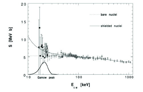
Figure 4: The measured energy dependence of the astrophysical S(E) factor for the ³He(³He,2p)⁴He reaction [35]. The solid curve is a fit to the data including the electron shielding parameters deduced by Aliotta et al. [20] from a study of the ³He(d,p)⁴He reaction; the dotted curve represents $S(E)$ for the bare nuclear interaction, extracted from the solid curve by removing the effects of the electron shielding.

Studies conducted in laboratories at the earth’s surface of very low energy thermonuclear reactions are limited predominantly by background effects of cosmic rays in the detectors, leading typically to more than 10 background events per hour. Conventional passive or active shielding around the detectors can only partially reduce the problem of cosmic-ray background. The best solution is to install an accelerator facility in a laboratory deep underground. As a pilot project, a 50 kV accelerator facility has been installed in the underground laboratory at Gran Sasso, where the flux of cosmic–ray muons is reduced by a factor 10⁶ compared with the flux at the surface (Fiorentini et al. [34]). This unique project, called LUNA (Laboratory for Underground Nuclear Astrophysics), was designed primarily for a renewed study of the reaction ³He(³He,2p)⁴He at low energies, aiming to reach the solar Gamow peak at $E_{0}\pm\Delta$/2 = 21$\pm$5 keV. This goal has been reached (Bonetti et al. [35]) with a detected reaction rate of about 1 event per month at the lowest energy, $E$ = 16 keV, with $\sigma$ = 20 fb or 2 $\times$ 10^-38 cm². Thus, the cross section of an important fusion reaction of the hydrogen-burning proton-proton chain has been directly measured for the first time at solar thermonuclear energies (Fig. 4): extrapolation is no longer needed in this reaction. Across the Gamow peak, after correction for electron shielding (see Eq. (6) and its associated text) their measured data can be characterized by [35]

$S$(0) = 5.32 $\pm$ 0.08 MeV–barns

$S^{\prime}$(0) = -3.7 $\pm$ 0.6 barns.

4.4 The ³He ($\alpha,\gamma$) ⁷Be reaction

The relative rates of the ³He(³He,2p)⁴He and ³He($\alpha,\gamma$)⁷Be reactions determine the branching ratio between the ppI and ppII+ppIII terminations of the pp–chain (see Figure 1). The former produces only the low energy p+p$\to$d+e${}^{+}+\nu_{e}$ neutrinos ($E_{\nu}\leq$ 420 keV), while the latter produce ⁷Be electron capture neutrinos and the high–energy ⁸B neutrinos ($E_{\nu}^{max}\sim$ 14.02 MeV), the neutrinos measured in the Homestake, SNO and Super-Kamiokande experiments.

Measurements of the ³He($\alpha,\gamma$)⁷Be reaction (six via measurements of the direct–capture gamma rays and three via measurements of the residual ⁷Be activity) were reviewed by a study group at the INT in 1997 (Section V in Ref. [29]), with the result that –

$S(0)_{DirectCapture}$= 0.507 $\pm$ .016 keV–b

$S(0)_{ResidualActivity}$= 0.572 $\pm$ .026 keV–b

$S(0)_{TotalDataSet}$= 0.533 $\pm$ .013 keV–b.

This study group concluded [29] that the grouping of the two data sets (direct vs. activity) around two different centroids “suggests the possible presence of a systematic error in one or both of the techniques. An approach that gives a somewhat more conservative evaluation of the uncertainty is to … determine the weighted mean of those two results (the direct–capture and residual-activity data sets). In the absence of information about the source and magnitude of the excess systematic error, if any, an arbitrary but standard prescription can be adopted in which the uncertainties of the means of the two groups (and hence of the overall mean) are increased by a common factor of 3.7 (in this case) to make $\chi^{2}$=0.46 for one degree of freedom, equivalent to making the estimator of the weighted population variance equal to the weighted sample variance. The uncertainty in the extrapolation is common to all the experiments and is likely to be only a relatively minor contribution to the overall uncertainty. The result is our recommended value for an overall weighted mean:

$S_{34}$(0) = 0.53 $\pm$ .05 keV–b.”

Now that the ⁷Be(p,$\gamma$)⁸B reaction rate seems to be on a firmer footing (see Section 4.5 below), the ³He($\alpha,\gamma$)⁷Be reaction rate, because of the inconsistency of the direct–capture and ⁷Be activity results, has become the most important nuclear uncertainty in the solar neutrino problem. To try to resolve this issue, at least four new studies of the ³He($\alpha,\gamma$)⁷Be reaction rate are currently underway. The approaches include new direct-capture and activity measurements, as well as a Coulomb-dissociation experiment. A recent series of ⁷Be–activity measurements [36] at four energies in the range 420 $<$ $E_{cm}<$ 950 keV determines an extrapolated intercept of $S_{34}$(0) = 0.53 $\pm$ .02 $\pm$ .01 keV–b.

It should be noted that the ³He($\alpha,\gamma$)⁷Be reaction exhibits a particularly simple, non–resonant behavior from its threshold to $E_{cm}$ $\sim$ 2.5 MeV, and its entrance-channel phase shifts are well determined over this energy range. Thus its energy dependence provides a good test of nuclear models. Section V of Ref. [29] provides a good review of theoretical work on this reaction.

4.5 The ³He(p,e${}^{+}\nu_{e}$)⁴He reaction

The “hep” reaction proceeds through the same weak–interaction as the pp reaction (Section 4.1, above), and as such its cross section factor would be expected to be orders of magnitude smaller than for the ³He(³He,2p)⁴He and ³He($\alpha,\gamma$)⁷Be reactions and of no interest as a significant termination for the pp–chain. However this weak branch produces energetic neutrinos ($E_{\nu}^{max}$ = 18.77 MeV) that extend beyond the endpoint of the ⁸B neutrino spectrum, so that in principle a weak flux could be detected. Both SNO and Super–Kamiokande have placed interesting limits on this flux; see Section 5, below.

The nuclear physics of this reaction is rather subtle: in a naive shell–model description, the incident proton would, by the Pauli exclusion principle, occupy a state orthogonal to the two s–shell protons in ³He. In the allowed approximation, the conversion of the proton to a neutron by the weak interaction would then produce a state orthogonal to the naïve s–shell ⁴He ground state. This suggests that smaller components in the nuclear wave function and corrections such as exchange currents might be unusually important in determining the cross section. For this reason theoretical uncertainties in estimating the rate are considerably larger than in pp beta–decay, despite modern few-body techniques that can be applied to the continuum four–body problem [37]. The most recent evaluation of the rate of this weak-interaction reaction [27] gives an S–factor of

$S_{hep}$(0) = (8.6 $\pm$ 1.3)$\times$10^-20 keV b,

corresponding to a hep termination branch for the pp–chain of 2.5$\times$10^-7 and a hep neutrino flux of $\Phi_{hep}$ = 7.9$\times$ 10³ cm^-2 s^-1 in BP04 [9].

Other ³He–burning reactions: The S–factor $S(0)$ for ³He(d,p)⁴He is comparable in magnitude to that for ³He(³He,2p)⁴He reaction, while the much smaller relative abundance of deuterium compared to ³He (d/³He $\mathrel{\hbox to0.0pt{\lower 4.0pt\hbox{\hskip 1.0pt$\sim$}\hss}\raise 1.0pt\hbox{$<$}}$ 10${}^{-12})$ more than compensates for the higher ³He+³He Coulomb barrier. (Deuterium has a very short lifetime $\sim$ 1 sec in the solar core. The ³He lifetime increases sharply with decreasing temperature, but is typically $\sim$10⁶ years in the hotter central core of the sun [33].) The net result is that the ³He(d,p)⁴He reaction accounts for less than 0.1$\%$ of ³He–burning in the solar interior.

4.6 The ⁷Be (e^-, $\nu$)⁷Li reaction

The neutral–atom lifetime and the branching ratio (the ratio of the transition rate to the first excited state ⁷Li^∗ to the total ⁷Li${}^{\ast}+^{7}$Li_gs rate) for the electron–capture decay of ⁷Be is well determined (see Table 7.6 in ref. [38]):

$\tau_{1/2}$ = 53.22 $\pm$ 0.06 days

$\omega$(⁷Li^∗)/ $\omega$(total) = (10.44 $\pm$ 0.06) $\%$.

However, one does not want the neutral–atom lifetime, but the lifetime for the conditions of the temperature and density in the solar interior – which determine the ionization state and the electron density governing this electron–capture decay rate.

Bahcall and Moeller [39] evaluated the rate for capture of a continuum electron as well as the contribution from bound–state capture in Be ions that are not totally ionized. While continuum capture dominates, inclusion of bound–state capture increases the rate by about 22$\%$. They found

$$\begin{array}[]{ll}R(^{7}Be+e^{-})=5.60\times 10^{-9}(\rho/2)(1+X_{H})T_{6}^{-1/2}\\ \hskip 65.44142pt\times[1+0.004(T_{6}-16)]s^{-1}.\end{array}$$ (18)

Gruzinov and Bahcall [40] used the density matrix formalism (e.g., Feynman [41]) in an alternative calculation of the rate. The result from this approach, which does not separate bound–state capture from continuum capture, agrees with Eq. (18) to better than 1$\%$.

4.7 The ⁷Be (p,$\gamma$)⁸B reaction

While the pp–III branch plays only a very minor role (0.013 $\%$) in solar energy production, the decay of the ⁸B produced in the⁷Be(p,$\gamma$) reaction is directly responsible for the production of essentially all of the solar neutrinos of interest to the SNO and Super-Kamiokande detectors. Motivated by interest in quantitatively understanding the solar neutrino fluxes measured in these detectors, experimentalist have mounted five new direct measurements of the ⁷Be(p,$\gamma$) reaction in the last decade, as well as a number of indirect measurements in which the rate is deduced either via the strength of a proton–transfer reaction or via Coulomb dissociation of a ⁸B beam.

Except for the original Kavanagh measurement of the high–energy positrons [42], the direct ⁷Be(p,$\gamma$) experiments have measured the reaction cross section by detecting the delayed alpha-particles, emitted following the $\beta$–decay of ⁸B ($\tau_{1/2}$ = 0.77 s) to ⁸Be. The five modern, low–energy ($E_{cm}<$ 425 keV) measurements [43, 44, 45, 46, 47] are consistent with each other, and when each is fit with the same theoretical model (e.g., DB94 [48]) they generate a weighted average of 21.4 $\pm$ 0.5 eV b [47]. However, there is an additional uncertainty introduced by the variations between models that can be fit to the data and then used to perform the extrapolation to $S_{17}$(0). Junghans et al. [47] compare 12 model calculations (their Fig. 16) all of which cluster around a central value of $\sim$22 $\pm$ 0.8 eV b. (See also Jennings et al. [49].) Junghans et al. combine these experimental and theoretical uncertainties as

$S_{17}$(0) = 21.4 $\pm$ 0.5 (exp) $\pm$ 0.6 (theory) eV b.

An important systematic uncertainty in these direct experiments has been the thickness and composition of the ⁷Be targets. To circumvent this issue an experiment is currently in its final planning stages at ORNL, which will utilize a ⁷Be beam incident on a hydrogen gas target [50]. (Of course, this will introduce other, but different, systematic issues, such as the distribution of the hydrogen gas in the windowless target and the charge-state distribution of the recoiling ⁸B nucleus in the recoil separator.) Two other proposed methods for avoiding the ⁷Be–target issues are indirect measurements of the reaction rate by (a) proton–transfer reactions or (b) the Coulomb dissociation (CD) of accelerated ⁸B ions:

(a) Transfer–reaction experiments [51] have been used to extract the asymptotic normalization coefficients (ANCs) from the reactions ¹⁰B(⁷Be,⁸B)⁹Be and ¹⁴N(⁷Be,⁸B)¹³C coupled with measurements of the ANCs for the ¹³C(p,$\gamma)$ and ⁹Be(p,$\gamma)$ reactions. The ANCs from these reactions determine the behavior of the tail of the ⁷Be+p wave function in the peripheral region that dominates capture reactions in such loosely bound nuclei. This method has been checked by comparing an ANC measurement of the ¹⁶O(³He,d)¹⁷F reaction with direct ¹⁶O(p,$\gamma)^{17}$F measurements, yielding agreement at the level of 9$\%$ [52]. The ANC analysis of the ¹⁰B(⁷Be,⁸B)⁹Be and ¹⁴N(⁷Be,⁸B)¹³C reactions by Azhari et al. [51] gave $S_{17}$(0) = 17.3 $\pm$ 1.8 eV b. An ANC analysis [53] of a number of ⁸B break–up studies (involving a variety of energies and targets) yielded a value of $S_{17}$(0) = 17.4 $\pm$ 1.5 eV b. However, it should be noted that a different, separate analysis [54, 55] of the ¹²C(⁸B,⁷Be)¹³N break–up reaction gave $S_{17}$(0) = 21.2 $\pm$ 1.3 eV b, indicating that substantial uncertainties remain in the interpretation of the measurements.

(b) Several ⁸B Coulomb–dissociation experiments (in which the break–up products are measured at very forward angles, corresponding to very large impact parameters and hence very small nuclear contributions) have been carried out for ⁸B beam energies from 52 to 254 MeV/nucleon. The four most recent Coulomb dissociation experiments [56, 57, 58, 59] deduce $S_{17}$(0) values in the range from 17.8 to 20.6 eV b. In the absence of a separate calibration of the CD method, at this time the comparison of the these ⁸B CD measurements with the direct ⁷Be(p,$\gamma)$ cross section measurements may be more important as a check on the level of validity of the CD method for determining (p,$\gamma)$ S–factors. Such a check is important in assessing CD for other cases where direct measurements may not be possible.

4.8 The Carbon–Nitrogen Cycle

Hydrogen burning via the CN–cycle (Fig. 2) accounts for less than 2$\%$ of the ⁴He produced in the sun. In their analysis of the status of the various nuclear reactions in this cycle, the 1997 INT study group [29] concluded that by far the most significant uncertainty in this cycle was the poorly defined role of the subthreshold resonance ($E_{cm}$ = -504 keV) in the extrapolation of the measured rate of the ¹⁴N(p,$\gamma)^{15}$O reaction. This reaction is $\sim$100 times slower than the other reactions in the CN–cycle and therefore determines the overall rate of this cycle. Based on their analysis of the data of Lamb $\&$ Hester [60] and Schröder et al. [61], the INT workshop participants recommended $S_{tot}$(0) = $3.5_{-2.0}^{+1.0}$ keV b, and emphasized the need for new experiments to improve our understanding of the ¹⁴N(p,$\gamma)^{15}$O reaction. Subsequently, in a further R–matrix reanalysis of the Schröder data, Angulo and Descouvement [62] extracted a reduced proton width for the subthreshold resonance corresponding to the 6.79–MeV state that was much smaller than the one used in the original Schröder analysis. This smaller reduced proton width resulted in a value of $S_{tot}$(0) = 1.77 $\pm$ 0.20 keV b for this reaction [62].

Recently, preliminary results have become available from two new, independent measurements of the rates for each of the gamma–ray transitions for the ¹⁴N(p,$\gamma)^{15}$O reaction, at the LENA (UNC–TUNL) facility and at the LUNA (Bochum–GranSasso) facility. The LENA measurements [63] utilized an implanted target (¹⁴N atoms implanted in 0.5–mm thick Ta backings) and were carried out down to $E_{cm}$ = 145 keV. The LUNA measurements [64] utilized both a solid target (for $E_{cm}\geq$ 130 keV) and a differentially–pumped N₂ gas target (for $E_{cm}\geq$ 70 keV). These LENA and LUNA data sets are in good agreement, well within their statistical uncertainties, and when combined with a remeasurement [65] of the lifetime of the subthreshold state at $E_{x}$ = 6.79 MeV, these new measurements indicate a factor of $\sim$2 reduction in the $S_{tot}$(0) value for this reaction, to 1.67 keV b, compared to the Schröder value of 3.5 keV b [61, 29]. (Preliminary reports for these two data sets indicate statistical uncertainties of $\sim$ 5$\%$ and systematic uncertainties of $\sim$ 9$\%$ in their determination of $S_{tot}$(0). However, it should be noted that the analysis of the 70–keV LUNA data point is not yet complete.)

A preliminary examination [63, 64] of the consequences of this factor of $\sim$2 reduction in the rate of the ¹⁴N(p,$\gamma)^{15}$O reaction finds (a) a corresponding factor of $\sim$2 reduction in the CN component of the solar neutrino flux and (b) an increase of $\sim$1 Gyr in globular cluster ages based on turn–off points from the main–sequence. When the data are final, the effects on detailed SSM neutrino flux predictions can be evaluated more quantitatively.

5 Solar Neutrino Fluxes: Theory and Experiment

The nuclear cross sections discussed here, together with other solar model parameters (e.g., abundances, the solar age), can be incorporated into solar model calculations, leading to predictions that can be verified in helioseismology or neutrino flux measurements. The principal neutrino fluxes from the pp chain are the pp and ⁸B beta–decay sources and the line sources (broadened by about 2 keV from thermal effects) from electron capture on ⁷Be. As seen from Figure 1, one of the reasons for the importance of these fluxes is that they provide a direct test of the competition among the ppI, ppII, and ppIII cycles that comprise the pp chain: the ⁷Be and ⁸B neutrinos tag the ppII and ppIII cycles, respectively, while the pp neutrinos then determine the total rate of fusion in the sun. This competition is an important check on the SSM, specifically its prediction of the sun’s central core $T_{c}$. For example, the ⁸B flux is found to vary as $\sim$ $T_{c}^{24}$ when solar model input parameters are varied (while conserving the luminosity), while the flux ratio $\phi(^{7}$Be)/$\phi(^{8}$B) $\sim$ $T_{c}^{-12}$. The precision with which these fluxes can be predicted in the SSM is also crucial to current efforts to better determine the parameters governing solar neutrino oscillations.

Results from the most recent Bahcall and Pinsonneault SSM (BP04) [9] are summarized below, where E10 = 10¹⁰:

Source	BP04 (cm${}^{-2}s^{-1})$	BP04+ (cm${}^{-2}s^{-1})$
pp	5.94(1$\pm$0.01) E10	5.99 E10
pep	1.40(1$\pm$0.02) E8	1.42 E8
hep	7.88(1$\pm$0.16) E3	8.04 E3
7Be	4.86(1$\pm$0.12) E9	4.65 E9
8B	5.79(1$\pm$0.23) E6	5.26 E6
13N	5.71(1$\pm$0.36) E8	4.06 E8
15O	5.03(1$\pm$0.41) E8	3.54 E8
17F	5.91(1$\pm$0.44) E6	3.97 E6

These results reflect the dominance of the ppI cycle in the pp–chain for present–day solar conditions: $\sim$ 85$\%$ of the sun’s energy in generated via this path. The ppII ($\sim$15$\%$) and ppIII ($\sim$0.02$\%$) account for the remainder. Approximately 1.7$\%$ of ⁴He synthesis occurs via the CNO cycle. Cross section uncertainties lead to substantial ranges in the predicted fluxes.

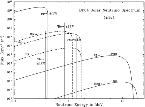
Figure 5: The solar neutrino spectrum of BP04 [9].

The cross section uncertainties discussed in this paper are included in the overall model uncertainties quoted for BP04, which uses older element abundances from Grevesse and Sauval [66]. Also shown are the results for BP04+, a calculation identical to BP04, but using more recent analyses of the solar surface abundances (C, N, O, Ne, Ar) of Allende Prieto et al. [67]. Contributing to the uncertainties in extracting solar surface abundances are systematics due to blending of atomic lines and uncertainties in modelling the solar atmosphere. The Allende Prieto et al. abundances substantially lower the surface heavy element to hydrogen ratio (from 0.0229 to 0.0176), which leads to a shallower convective zone and discrepancies with helioseismology. The BP04+ neutrino fluxes reflect a shift in the pp chain toward the ppI cycle because the lower metalicity produces a somewhat cooler sun. Because of its temperature sensitivity, the ⁸B flux shows the largest change among pp fluxes, a 10$\%$ decrease. The lower abundances for C, N, and O directly influence CN–cycle neutrino fluxes, as does the lower value for $T_{c}$, leading to changes on the order of 40$\%$. BP04 neutrino spectrum is shown in Fig. 5. The ⁸B neutrino spectrum deviates slightly from an allowed shape because the final ⁸Be state is a broad resonance.

The prospect of directly probing the thermonuclear reactions occurring in the solar core helped to motivate Ray Davis and his colleagues [68] to mount their pioneering chlorine solar neutrino experiment. Sited nearly a mile underground in the Homestake Mine to avoid cosmic ray–induced backgrounds, this radiochemical detector operated almost continuously from its construction in 1967 until 2002. The experiment exploited a reaction, ³⁷Cl($\nu_{e}$,e${}^{-})^{37}$Ar, that had been first suggested by Pontecorvo [69] and by Alvarez [70]. The technique involved the collection of the product ³⁷Ar ($\tau_{1/2}\sim$ 35 d) from a tank containing 0.61 kiloton of perchloroethylene (C₂Cl${}_{4})$. Gas was removed from the tank about every two months by a helium purge, then circulated through a condenser, a molecular sieve, and a charcoal trap cooled to the temperature of liquid nitrogen. The resulting efficiency for collecting the ³⁷Ar was high, typically greater than 95$\%$, as was demonstrated by the recovery of known amounts of the carrier gases ³⁶Ar or ³⁸Ar that were introduced at the start of each run. After extraction, the trap was heated and swept by helium. The extracted gas was passed through a hot titanium filter to remove reactive gases, and the argon was then separated from other noble gases by gas chromatography. The purified argon was loaded into a miniaturized gas proportional counter, where the subsequent electron capture on ³⁷Ar was measured through the 2.82 keV of energy that is released as the atomic electrons in ³⁷Cl adjust to fill the K–shell vacancy. The counting typically continued for about a year ($\sim$ 10 half lives).

After accounting for small contributions from neutron– and comic–ray–induced backgrounds, Davis determined a solar neutrino production rate of $\sim$ 0.5 ³⁷Ar atoms/day in the tank. Despite the low counting rate, the final results for the experiment achieved an impressive accuracy, 2.56 $\pm$ 0.16 (stat) $\pm$ 0.16 (syst) SNU, where a Solar Neutrino Unit (SNU) is 10^-36captures/³⁷Cl atom/s [71]. The chlorine experiment is primarily sensitive to ⁸B neutrinos ($\sim$ 76$\%$), which can induce the strong super–allowed transition to the 4.99 MeV state in ³⁷Ar, and ⁷Be neutrinos ($\sim$16$\%$), which are sufficiently energetic to overcome the 814 keV threshold of the ground–state transition. The discrepancy between the chlorine results and the SSM predictions (8.5 $\pm$ 1.8 SNU for BP04) was the genesis of the solar neutrino problem.

Two similar radiochemical experiments, SAGE and GALLEX, began solar neutrino measurements in January 1990 and May 1991, respectively. These exploited the reaction ⁷¹Ga($\nu_{e}$,e${}^{-})^{71}$Ge which, because of the strength and low Q–value for the ground–state transition, is primarily sensitive to the low–energy pp neutrinos. SAGE, which employed 60 tons of liquid Ga metal, continues to operate in the Baksan Neutrino Observatory, under 4700 mwe of shielding provided by Mount Andyrchi in the Caucasus. GALLEX and its successor GNO, which used 30.3 tons of Ga as GaCl₃ in a hydrochloric acid solution, operated until very recently in the Gran Sasso Laboratory in Italy (3300 mwe).

The primary challenge in both experiments is the more complicated chemistry of Ge extraction, which is done about every three weeks. In SAGE the Ge is separated by vigorously mixing into the gallium a mixture of hydrogen peroxide and dilute hydrochloric acid. This produces an emulsion, with the Ge migrating to the surface of the emulsion droplets where it is oxidized and dissolved by hydrochloric acid. The Ge is extracted as GeCl₄, purified and concentrated, synthesized into GeH₄, and further purified by gas chromatography. The overall efficiency, determined by introducing a Ge carrier, is typically 80$\%$. In GALLEX/GNO the Ge is recovered as GeCl₄ by bubbling nitrogen through the solution and then scrubbing the gas through a water absorber. The Ge is further concentrated and purified, and finally converted into GeH₄. The overall extraction efficiency is typically 99$\%$.

In both experiments the GeH₄ is inserted into miniaturized gas proportional counters, carefully designed for radiopurity, and the ⁷¹Ge is counted as it decays back to ⁷¹Ga ($\tau_{1/2}$ = 11.43 d). As in the case of ³⁷Ar, the only signal is the energy deposited by Auger electrons and X rays that accompany atomic rearrangement in Ga. Both K and L captures can be detected. Intense ⁵¹Cr neutrino sources were used to calibrate both detectors [72]. SAGE is currently conducting a test calibration with a ³⁷Ar source, in preparation for an anticipated repeat of this experiment with $\sim$ 2 MCi of ³⁷Ar [73].

The most recent results of SAGE give a counting rate of 66.9 $\pm$ 3.9 (stat) $\pm$ 3.6 (syst) SNU [74], while the GALLEX/GNO result is 69.3 $\pm$ 4.1 (stat) $\pm$ 3.6 (syst) SNU [75]. The rates are in good agreement, but well below the SSM prediction (131 $\pm$ 11 SNU in BP04).

Two types of direct–counting experiments have also been done, using the water Cerenkov detectors Kamiokande and Super–Kamiokande and the heavy-water detector SNO (Sudbury Neutrino Observatory). Kamiokande, a 4.5–kiloton cylindrical imaging water Cerenkov detector, was originally designed for proton decay but was later reinstrumented to detect ⁸B solar neutrinos. (The improvements included sealing the detector against radon inleakage and recirculating the water through ion exchange columns.) It operated for nearly a decade (1987–95) detecting solar neutrinos by the Cerenkov light produced by recoiling electrons in the reaction $\nu_{x}$ + e $\to\nu_{x}^{\prime}$ + e^′. Both electron and heavy–flavor neutrinos contribute to the scattering, with $\sigma(\nu_{e})$/$\sigma(\nu_{\mu})\sim$ 7. The threshold of the detector was initially 9.5 MeV but was ultimately lowered to 7 MeV, due to Kamiokande III improvements in electronics and the addition of wavelength shifters to improve PMT light collection. The inner 2.14 kilotons of water was viewed by 948 50–cm photomultiplier tubes (PMTs), which provided 20$\%$ photocathode coverage. An additional 123 PMTs viewed the surrounding 1.5m of water, which served as an anticounter. The fiducial volume employed for solar neutrino measurements was the central 0.68 kilotons, the region most isolated from the high–energy gamma rays generated in the surrounding rock walls of the Kamioka mine. Kamiokande found a ⁸B neutrino flux of (2.80 $\pm$ 0.19 $\pm$ 0.33) $\times$ 10⁶/cm²s [76], 48$\%$ of the BP04 SSM prediction of (5.79 $\pm$ 1.33) $\times$ 10⁶/cm²s.

The experiment was remarkable in several respects. It was the first to measure solar neutrinos in real time. It exploited the sharp forward peaking of the scattered electrons, in the direction of the incident neutrino, to extract solar neutrino events from a significant but isotropic background. The “pointing” of events back to the sun provided the first direct evidence that neutrinos originated from the sun.

Super–Kamiokande, the massive 50–kton successor to Kamiokande, collected 1496 days of solar neutrino data over its first run, from May 1996 through July 2001. With its high PMT coverage (40$\%$), lower threshold ($\sim$ 5 MeV), and much larger fiducial volume (22.5 ktons), Super–Kamiokande collected data at a rate $\sim$ 100 times faster than that of its predecessor, Kamiokande. The result was an extraordinary set of precise measurements of the flux, recoil electron spectrum, and seasonal (earth’s orbital eccentricity) and day/night (earth regeneration of neutrinos) time variations of the solar neutrinos. The experiment placed a significant constraint on the hep flux ($<$ 7.3 $\times$ 10⁴/cm²s, a limit about 10 times the BP04 prediction) and on various exotic neutrino properties, such as magnetic moments. Super–Kamiokande’s ⁸B neutrino flux result is (2.35 $\pm$ 0.19 $\pm$ 0.33) $\times$ 10⁶/cm²s [77], 41$\%$ of the BP04 prediction.

The SNO detector was built deep in the Creighton $\#$9 nickel mine in Sudbury, Ontario, for the purpose of determining the flavor content of the ⁸B solar neutrino flux. A central acrylic vessel containing one kiloton of heavy water is surrounded by 5m (7 ktons) of light water to shield the inner volume from neutrons and gammas. The detector is viewed by 9500 20–cm PMTs, providing 56$\%$ coverage.

The heavy water allows the experimenters to exploit three reactions with varying flavor sensitivities

$\nu_{e}$ + d $\to$ p + p + e^-  (CC: charged current)

$\nu_{x}$ + d $\to\nu_{x}^{\prime}$ + n + p   (NC: neutral current)

$\nu_{x}$ + e^- $\to\nu_{x}^{\prime}$ + e^-′     (ES: elastic scattering)

As the Gamow–Teller threshold for the CC reaction is concentrated close to the p + p threshold of 1.44 MeV, most of the neutrino energy is transferred to the electron. Thus the CC electron spectrum provides a better probe of $\nu_{e}$ spectral distortions than does the ES electron spectrum.

The NC reaction, which is observed through the produced neutron, provides no spectral information, but does measure the total solar neutrino flux, independent of flavor. The SNO experiment has used two techniques for measuring the neutrons. In the initial SNO pure D₂O phase the neutron signal was capture on deuterium, which produces 6.25 MeV gammas. In a second phase 2.7 tons of salt was added to the heavy water so that Cl would be present to enhance the capture, producing 8.6 MeV gammas. The NC and CC events can be separated reasonably well because of the modest backward peaking ($\sim$1 – cos($\theta)$/3) in the angular distribution of the latter. This allowed the experimenters to determine the total and electron neutrino fraction of the solar neutrino flux. A third phase has begun in which direct neutron detection is provided in pure D₂O by an array of ³He–filled proportional counters.

The ES, which we noted previously measures electron and heavy-flavor neutrinos, but with reduced sensitivity to the latter, is the same reaction exploited by Super–Kamiokande. Because the SNO volume is smaller, the SNO ES statistics are reduced. However, the lower SNO backgrounds lead to a smaller systematic error, so that the overall the SNO and Super–Kamiokande sensitivities are comparable. Because the ES and CC scattered electrons are measured in the same detector, the ES reaction provides an important cross check on the consistency of the results from the CC and NC channel.

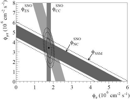
Figure 6: The flux of ⁸B solar neutrinos which have either $\mu$ or $\tau$ flavor vs. the corresponding flux of electron neutrinos, as deduced from the charge–current (CC), neutral–current (NC), and elastic–scattering (ES) reactions in the SNO heavy–water detector [78].

The SNO results are presented in Fig. 6. The deduced fluxes are [78]

$\phi_{CC}$ = (1.59 $\pm$ 0.08 $\pm$ 0.07) $\times$ 10⁶/cm²s

$\phi_{ES}$ = (2.21 $\pm$ 0.28 $\pm$ 0.10) $\times$ 10⁶/cm²s

$\phi_{NC}$ = (5.21 $\pm$ 0.27 $\pm$ 0.38) $\times$ 10⁶/cm²s

The total flux (NC) is in agreement with the SSM prediction, but the CC results indicate that almost 70$\%$ of the solar neutrinos arrive on earth as heavy–flavor neutrinos. The ES results are in excellent accord with this conclusion, as Fig. 6 shows, as well as with the Super-Kamiokande results. The data rule out the hypothesis of no flavor change at greater than 7$\sigma$.

6 Conclusions

This paper has reviewed two problems. The first was the 70–year effort to understand solar energy generation and stellar evolution as a consequence of the thermonuclear reactions occurring in the interiors of stars. It led to collaborations between solar modelers, who constructed codes to describe the evolution of our sun and to predict its helioseismology and neutrino production, and laboratory experimentalists, who provided the nuclear reaction data essential to the SSM. The second was the nearly 40–year program to measure the flux, flavor, and spectrum of solar neutrinos. This effort began with the pioneering experiment of Ray Davis, Jr. and his collaborators at Homestake, and led to the current generation of sophisticated active detectors, SNO and Super–Kamiokande.

Both programs required great patience—years of effort to refine the SSM and to develop better solar neutrino detection techniques—before it became clear that the resolution of the solar neutrino problem had to be new physics. That resolution included a new phenomenon, matter enhancement of neutrino oscillations, which altered our view of neutrino oscillations and opened up new experimental tests, such as spectral distortions and day–night effects. This further motivated the development of robust detectors like SNO and Super–Kamiokande.

The conclusion that was reached after decades of work is quite profound: the solar neutrino discrepancy first identified by Davis is due to new particle physics, neutrino oscillations. This phenomenon lies outside the minimal standard model, requiring massive neutrinos and a nontrivial relationship between mass and weak–interaction eigenstates. Analyses that take into account not only the solar neutrino data described above, but also the KamLAND reactor neutrino data [79], conclude [80]

$\delta$m${}_{21}^{2}$ = m${}_{2}^{2}$-m${}_{1}^{2}\quad\sim$ (8.2 $\pm$ 0.3 $\pm$ 0.9) $\times$ 10^-5 eV²

tan${}^{2}\theta_{12}\quad\sim$ 0.39 $\pm$ 0.05 $\pm$ 0.15,

where $\theta_{12}$ is the neutrino mixing angle and m₁ and m₂ the mass eigenvalues. The KamLAND data are very important in further constraining the mass difference and thus the vacuum oscillation length.

This explanation of the solar neutrino puzzle raises new questions. What accounts for the scale of neutrino masses, a scale so different from other standard-model fermion masses? Why are neutrino mixing angles large? (The corresponding atmospheric–neutrino mixing angle $\theta_{23}$ is maximal, to within measurement uncertainties.) There are many parameters in the neutrino mixing matrix not yet determined. These include the absolute scale of neutrino mass, the hierarchy (where the nearly degenerate pair of neutrinos that participate in solar neutrino oscillations are lighter than or heavier than the third neutrino), the size of the third mixing angle $\theta_{13}$, the charge conjugation properties of neutrinos (that is, whether the masses are generated from Majorana or Dirac mass terms), and the size of the CP–violating phases that appear in the mixing matrix. The answers to these questions could help point the way to important extensions of the standard model.

One of the most remarkable outcomes of the solar (and atmospheric) neutrino problems is that the neutrino mass differences that emerged are in a range accessible to terrestrial experiments with accelerator and reactor neutrinos, such as KamLAND. Despite the importance of future terrestrial experiments—such as double beta decay searches for Majorana masses and long-baseline neutrino experiments to look for CP violation—solar neutrinos still have an important role to play. For the foreseeable future (e.g., until beta beams are developed), solar neutrinos will remain our only intense source of electron neutrinos. Some future goals that might be reached by exploiting these neutrinos include [81]:

* A low–energy solar neutrino measurement to test the consequences of a large $\theta_{12}.$ One feature of the accepted LMA (Large Mixing Angle) neutrino oscillation explanation of current data is that the survival probability for low energy neutrinos is substantially higher than that for the ⁸B electron neutrinos measured in SNO’s CC channel. Verifying this prediction is important.

* Future high–statistics pp solar neutrino experiments to improve our knowledge of $\theta_{12}.$ Solar neutrino experiments are the primary source of information on $\delta$m${}_{12}^{2}$ and $\theta_{12}$. While KamLAND has helped to narrow the LMA solution region in $\delta$m${}_{12}^{2}$, neither it nor Borexino will appreciably improve our knowledge of the mixing angle. A pp solar neutrino measurement with an uncertainty of 3$\%$ would constrain $\theta_{12}$ with an accuracy comparable to that possible with the entire existing set of solar neutrino data. Thus a goal of next–generation pp solar neutrino experiments is to achieve 1$\%$ uncertainty, thus substantially tightening the constraints on $\theta_{12}$.

* Precise flux measurements of the low–energy (pp and⁷Be) solar neutrinos to improve limits on sterile neutrinos coupling to the electron neutrino. Sterile neutrinos with even small couplings to active species can have profound cosmological effects. The coupling of $\nu_{e}$s to sterile states can be limited by CC and NC measurements with an accurately known neutrino source. KamLAND (together with the SNO CC and NC data) should ultimately limit the sterile component of ⁸B neutrinos to $\sim$ 13$\%$. This bound can be improved by measuring the NC and CC interactions of pp and ⁷Be neutrinos to accuracies of a few percent. In general one expects the sterile component of solar neutrino fluxes to be energy dependent. Thus low–energy solar neutrino experiments are an important part of such searches.

* Preliminary estimates indicate that limits on the neutrino magnetic moment could be improved by an order of magnitude in future pp neutrino ES experiments. A neutrino magnetic moment will generate an electromagnetic contribution to neutrino ES, distorting the spectrum of scattered electrons. The effect, relative to the usual weak amplitude, is larger at lower energies, making a high-precision pp solar neutrino experiment an attractive testing ground for the magnetic moment. The strongest existing laboratory limit, $\mu(\nu_{e})<$ 1.5 $\times$ 10^-10 Bohr magnetons, could be improved by an order of magnitude in a 1$\%$ experiment.

* Future pp solar neutrino experiments to probe CPT violation with an order of magnitude more sensitivity than has been achieved in the neutral kaon system. As neutrinos are chargeless, they provide an important testing ground for CPT violation. If CPT is violated, the neutrino mass scale and mass splittings will differ between neutrinos and antineutrinos. (This has been offered as a possible explanation of the LSND neutrino oscillation results.) A high precision measurement of the pp $\nu_{e}$survival probability is an important component of CPT violation searches. In some models this will test CPT violation at a scale $<$ 10^-20 GeV, which can be compared to the present bound from the neutral kaon system, $<$ 4.4 $\times$ 10^-19 GeV.

* Solar neutrino detectors are superb supernova detectors. Many of the most interesting features in the supernova neutrino “light curve” are flavor specific and occur at late times, 10 or more seconds after core collapse. Because of their low thresholds, flavor specificity, large masses, and low backgrounds, solar neutrino detectors are ideal for following the neutrino emission out to late times. Solar neutrino detectors will likely be the only detectors capable of isolating the supernova $\nu_{e}$ flux during the next supernova. The 3 ms deleptonization burst, important in kinematic tests of neutrino mass, is mostly of this flavor. Electron–flavor neutrinos also control the isospin of the nucleon gas—the so called “hot bubble”—that expands off the neutron star. The hot bubble is the likely site of the r–process. Currently we lack a robust model of supernova explosions. The open questions include the nature of the explosion mechanism, the possibility of kaon or other phase transitions in the high density protoneutron star matter, the effects of mixed phases on neutrino opacities and cooling, possible signatures of such phenomena in the neutrino light curve, and signals for black hole formation. Supernovae are ideal laboratories for neutrino oscillation studies. One expects an MSW crossing governed by $\theta_{13}$, opening opportunities to probe this unknown mixing angle. The MSW potential of a supernova is different from any we have explored thus far because of neutrino–neutrino scattering contributions. Oscillation effects can be unravelled because the different neutrino flavors have somewhat different average temperatures. All of this makes studies of supernova neutrino arrival times, energy and time spectra, and flavor composition critically important. Finally, the detection of the neutrino burst from a galactic supernova will provide an early warning to optical astronomers: the shock wave takes from hours to a day to reach the star’s surface.

* Future solar neutrino experiments could provide crucial tests of the SSM. The delicate competition between the ppI, ppII, and ppIII cycles comprising the pp chain is sensitive to many details of solar physics, including the core temperature, the sun’s radial temperature profile, the opacity, and the metalicity. We have noted that this competition can be probed experimentally by measuring the ⁷Be flux (which tags the ppII cycle), the ⁸B flux (which tags the ppIII cycle), and the pp flux (which effectively tags the sum of ppI, ppII, and ppIII). Precise measurements of the pp and ⁷Be neutrino fluxes, combined with further improvements in nuclear cross section determinations, could significantly improve our understanding of current conditions in the solar core.

$\ast$ The CN neutrino flux is an important test of stellar evolution. The CN cycle is thought to control the early evolution of the sun, as out–of–equilibrium burning of C, N, and O powers an initial convective solar stage, thought to last about 10⁸ years. Furthermore, one of the key SSM assumptions equates the initial core metalicity to today’s surface abundances. A measurement of CN cycle neutrinos would quantitatively test this assumption. The recent controversy about surface elemental abundances provides additional motivation.

This work was supported in part by the US Department of Energy under grants DE-FG02-00ER-41132, DE-FC02-01ER-41187 (SciDAC), and DE-FG02-91ER-40609.

.

References

- [1] A.S. Eddington, Internal Structure of Stars (Cambridge Univ. Press, 1926) Chapter XI.
- [2] J.D. Burchfield, Lord Kelvin and the Age of the Earth (Science History Publications, 1975).
- [3] G. Gamow, Z. Phys. 52 (1928) 510.
- [4] R. d’E.Atkinson, F.G. Houtermans, Z. Phys. 54 (1928) 656.
- [5] C.F. vonWeizsãcker, Physik. Z. 38 (1937) 176.
- [6] C.F. vonWeizsãcker, Physik. Z. 39 (1938) 663.
- [7] H.A. Bethe, C.L. Critchfield, Phys. Rev. 54 (1938) 248.
- [8] H.A. Bethe, Phys. Rev. 55 (1939) 434.
- [9] J.N. Bahcall, M.H. Pinsoneault, Phys. Rev. Letts. 92 (2004) 121301.
- [10] E.M. Burbidge, G.R. Burbidge, W.A. Fowler, F. Hoyle, Rev. Mod. Phys. 29 (1957) 547.
- [11] D.D. Clayton, Principles of Stellar Evolution and Nuclear Synthesis, (McGraw–Hill, 1968).
- [12] C.E. Rolfs, W.S. Rodney, Cauldrons in the Cosmos, (University of Chicago Press, 1988).
- [13] W.A. Fowler, G.R. Caughlin, B.A. Zimmerman, Ann. Rev. Astron. Astrophys. 5 (1967) 525.
- [14] C. Angulo et al. (the NACRE collaboration), Nucl. Phys. A 656 (1999) 3.
- [15] E.E. Salpeter, Austral. J. Phys. 7 (1954) 373.
- [16] J.N. Bahcall, Ap. J. 143 (1966) 259.
- [17] H.J.K. Assenbaum, K. Langanke, C. Rolfs, Z. Phys. A327 (1987) 461.
- [18] S.A. Engstler et al., Phys. Lett. B202 (1988) 179.
- [19] F. Strieder et al., Naturwissenschraften 88 (2001) 461.
- [20] M. Aliotta et al., Nucl. Phys. A690 (2001) 790.
- [21] F. Raiola et al., Eur. Phys. J. A19 (2004) 283.
- [22] F. Raiola et al., (to be submitted).
- [23] E.E. Salpeter, Phys. Rev. 88 (1952) 547.
- [24] J.N. Bahcall and R.M. May, Ap. J. 155 (1969) 501.
- [25] X. Kong and F. Ravndal, Nucl. Phys. A 656 (1999) 421.
- [26] K.I.T. Brown, M.N. Butler, and D.B. Guenther, nucl–th/0207008/.
- [27] T.–S. Park et al., Phys. Rev. C 67 (2003) 055206.
- [28] R. Schiavilla et al., Phys. Rev. C 58 (1998) 1263.
- [29] E.G. Adelberger et al., Rev. Mod. Phys. 70 (1998) 1265.
- [30] G.M. Griffiths, M. Lal, C.D. Scarfe, Can. J. Phys. 41 (1963) 724.
- [31] G.J. Schmid et al., Phys. Rev. C 52 (1995) R1732.
- [32] C. Casella et al., Nucl. Phys. A706 (2002) 203.
- [33] P.D. Parker, J.N. Bahcall, W.A. Fowler, Ap. J. 139 (1964) 602.
- [34] G. Fiorentini et al., Z. Phys. A350 (1995) 289.
- [35] R. Bonetti et al., Phys. Rev. Lett. 82 (1999) 5205.
- [36] B.S. Nara Singh et al., Phys. Rev. Lett. (in press).
- [37] L.E. Marcucci et al., Phys. Rev. Lett. 84 (2000) 5959.
- [38] D.R. Tilley et al., Nucl. Phys. A708 (2002) 3.
- [39] J.N. Bahcall and C.P. Moeller, Ap. J. 155 (1969) 511.
- [40] A.V. Gruzinov and J.N. Bahcall, Ap. J. 490 (1997) 437.
- [41] R.P. Feynman, Statistical Mechanics, (Addison–Wesley, 1990) Chap. 2
- [42] R.W. Kavanagh, Nucl. Phys. 15 (1960) 411.
- [43] B.W. Filippone et al., Phys. Rev. Lett. 50 (1983) 412; Phys. Rev. C 28 (1983) 2222.
- [44] F. Hammache et al., Phys. Rev. Lett. 80 (1998) 928; Phys. Rev. Lett. 86 (2001) 3985.
- [45] F. Strieder et al., Nucl. Phys. A696 (2001) 219.
- [46] L.T. Baby et al., Phys. Rev. Lett. 90 (2003) 022501; Phys. Rev. C 67 (2003) 065805
- [47] A.R. Junghans et al., Phys. Rev. Lett. 88 (2002) 041101; Phys. Rev. C 68 (2003) 065803.
- [48] P. Descouvement and D. Baye, Nucl. Phys. A567 (1994) 341.
- [49] B.K. Jennings et al., Phys. Rev. C 58 (1998) 3711.
- [50] A.E. Champagne et al., ORNL-RIB No. 049.
- [51] A. Azhari et al., Phys. Rev. C 63 (2001) 055803.
- [52] C.A. Gagliardi et al., Phys. Rev. C 59 (1999) 1149.
- [53] L. Trache et al., Phys. Rev. Lett. 87 (2001) 271102.
- [54] B.A. Brown et al., Phys. Rev. C 65 (2002) 061601.
- [55] J. Enders et al., Phys. Rev. C 67 (2003) 064301.
- [56] T. Kikuchi et al., Phys. Lett. B391 (1997) 261; Eur. Phys. J. A 3 (1998) 213.
- [57] N. Iwasa et al., Phys. Rev. Lett. 83 (1999) 2910.
- [58] B. Davids et al., Phys. Rev. Lett. 86 (2001) 2750.
- [59] F. Schümann et al., Phys. Rev. Lett. 90 (2003) 232541.
- [60] W.A.S. Lamb and R.E. Hester, Phys. Rev. 108 (1957) 1304.
- [61] U. Schröder et al., Nucl. Phys. A467 (1987) 240.
- [62] C. Angulo and P. Descouvement, Nucl. Phys. A690 (2001) 755.
- [63] R. Runkle et al., (submitted to Phys. Rev. Lett.).
- [64] D. Bemmerer et al., (private communication).
- [65] P.F. Bertone et al., Phys. Rev. Lett. 87 (2001) 152501.
- [66] N. Grevesse and A.J. Sauval, SpaceSci. Rev. 85 (1998) 161.
- [67] C. Allende Prieto, D.L. Lambert and M. Asplund, Ap. J. 573 (2002) L137 and Ap. J. 556 (2001) L63.
- [68] R. Davis, Jr., D.S. Harmer, K.C. Hoffman, Phys. Rev. Lett. 20 (1968) 1205.
- [69] B. Pontecorvo, Chalk River Rep. PD–205 (1946) (unpublished).
- [70] L.W. Alvarez, Univ. Calif. Rad. Lab. Rep. UCRL–328 (1949) (unpublished).
- [71] B.T. Cleveland et al., Ap. J. 496 (1998) 505.
- [72] P. Anselmann et al., Phys. Lett. B342 (1995) 440; J.N. Abdurashitov et al., Phys. Rev. Lett. 77 (1996) 4708; W. Hampel et al., Phys. Lett. B420 (1998) 14.
- [73] V.N. Gavrin, private communication.
- [74] V.N. Gavrin et al., Nucl. Phys. B118 (2003) 39; and talk presented at the 8th Int. Conf. on Topics in Astroparticle and Underground Physics, Seattle, Sept. 2003.
- [75] T. Kirsten et al., Nucl. Phys. B118 (2003) 33; E. Bellotti, talk presented at the 8th Int. Conf. on Topics in Astroparticle and Underground Physics, Seattle, Sept. 2003.
- [76] Y. Fukuda et al., Phys. Rev. D 44 (1996) 1683.
- [77] S. Fukuda et al., Phys. Rev. Lett. 86 (2001) 5651; and Phys. Lett. B539 (2002) 179.
- [78] Q.R. Ahmad et al., Phys. Rev. Lett. 87 (2001) 071301; 89 (2002) 011301; and 89 (2002) 011302.
- [79] The KamLAND Collaboration, hep–ex/0406035/ and submitted to Phys. Rev. Lett.
- [80] J.N. Bahcall, M.C. Gonzalez–Garcia, and Carlos Pena–Garay, JHEP 0408 (2004) 016.
- [81] The Homestake Collaboration, W. C. Haxton et al., nucl-ex/0308018/.
.