Time-Dependent Response Calculations of Nuclear Resonances

Abstract

A new alternate method for evaluating linear response theory is formally developed, and results are presented. This method involves the time-evolution of the system using TDHF and is constructed directly on top of a static Hartree-Fock calculation. By Fourier transforming the time-dependent result the response function and the total probability amplitude are extracted. This method allows for a coherent description of static properties of nuclei, such as binding energies and deformations, while also providing a method for calculating collective modes and reaction rates. A full 3-D Cartesian Basis-Spline collocation representation is used with several Skyrme interactions. Sample results are presented for the giant multipole resonances of ¹⁶O, ⁴⁰Ca, and ³²S and compared to other calculations.

I Introduction

Typically, linear response theory equations are derived by adding a specific time-dependent perturbing function to the Hamiltonian, which is usually harmonic in time, resulting in a set of RPA-like equations. These equations are then solved, for a given energy, using several methods (see for example Refs. bertsch ; krewald ; liu ; SgII ) to give the response of the system to a specific collective excitation mode.

In this paper, a new alternate method is presented to calculate response theory. A specific time-dependent perturbing external piece is added to the static Hamiltonian to give a time-dependent total Hamiltonian, $H_{tot}(t)$. A static Hartree-Fock solution is then time-evolved using this $H_{tot}(t)$ in a time-dependent Hartree-Fock (TDHF) calculation. The time-dependent result is then Fourier transformed to give the response of the system for all energies. In this scheme one recovers both the response spectrum as well as the total transition probability amplitude corresponding to a given specific collective mode. Similar analyses of the long-time evolution of TDHF equations to study collective vibrations have been utilized in the past BF79 ; umar1 ; umar2 ; SCF01 ; SC03 , as well as extensions to study the damping of giant resonances BCT92 ; TU02 . The main advantage of this approach is that the dynamical response calculation is constructed directly on top of a static Hartree-Fock calculation and hence the static and dynamical calculations are calculated using the same Hamiltonian description. Therefore there is a complete consistency between the static ground state of the system and the response calculations. One can then provide a coherent description of static properties of nuclei and of dynamical properties. This is important for example in $\beta-$decay calculations of exotic nuclei, where reliable predictions are very sensitive to the deformation properties of the nucleus sorlin . Hence in this formalism consistent predictions of both the deformation and reaction rate properties are possible.

The static and dynamical Hartree-Fock calculations are performed using a 3-D Cartesian Basis-Spline collocation expansion umar3 ; umar4 . Properties of Basis-Splines include the practicality associated with coordinate-space lattice grids, while also providing accurate representations of the gradient operator and a good description of the continuum.

In Section II, the time-dependent evaluation of the response theory is discussed and shown to give the total transition probability. Numerical details and sample results are presented in Section III.

II Time-Dependent Response Theory

The response equations can be derived from a specific time-dependent perturbation functional of the TDHF equations fetter . To begin the proof a solution to the static Schrödinger equation is written as follows:

$${\widehat{H}}|\psi_{s}(0)\rangle=E|\psi_{s}(0)\rangle.$$ (1)

A time-dependent perturbing function is added to the static Hamiltonian:

$${\widehat{H}}_{tot}={\widehat{H}}+{\widehat{H}}_{ex}(t).$$ (2)

The external piece is defined as:

$${\widehat{H}}_{ex}(t) = {\widehat{F}}f(t)$$ (3)

$$= \left[\int d^{3}x\;{\widehat{n}}(\bm{x},t)F(\bm{x})\right]f(t),$$

where ${\widehat{n}}(\bm{x},t)$ is the number density operator and $F(\bm{x})$ corresponds to a one-body operator to excite a particular collective mode. The functions, $F(\bm{x})$ and $f(t)$ will be chosen later.

At some time $t=t_{0}$ the external piece of the Hamiltonian is turned on where $|{\bar{\psi}}_{s}(t)\rangle$ is the solution to the time-dependent Schrödinger equation:

$$\imath\hbar\frac{\partial}{\partial t}|{\bar{\psi}}_{s}(t)\rangle=\left[{\widehat{H}}+{\widehat{H}}_{ex}(t)\right]|{\bar{\psi}}_{s}(t)\rangle.$$ (4)

Here the subscript “$s$” refers to the Schrödinger picture. A solution of the following form is then constructed:

$$|{\bar{\psi}}_{s}(t)\rangle=e^{-\imath{\widehat{H}}t/\hbar}{\widehat{A}}(t)|\psi_{s}(0)\rangle,$$ (5)

where for $t\leq t_{0}$, ${\widehat{A}}(t)=1$. Using Eq. (4), the function ${\widehat{A}}(t)$ can be shown to be a solution to:

$$\imath\hbar\frac{\partial}{\partial t}{\widehat{A}}(t)={\widehat{H}}_{ex}^{I}(t){\widehat{A}}(t),$$ (6)

where the superscript “$I$” refers to the interaction picture, which reduces to the Heisenberg picture when ${\widehat{H}}_{ex}(t)=0$. The solution to Eq. (6) can be written iteratively as:

$${\widehat{A}}(t)=1-\frac{\imath}{\hbar}\int_{t_{0}}^{t}dt^{\prime}{\widehat{H}}_{ex}^{I}(t^{\prime})+...,$$ (7)

where the state vector is then given by:

$$|{\bar{\psi}}_{s}(t)\rangle=e^{-\imath{\widehat{H}}t/\hbar}|\psi_{s}(0)\rangle-\frac{\imath}{\hbar}e^{-\imath{\widehat{H}}t/\hbar}\int_{t_{0}}^{t}dt^{\prime}{\widehat{H}}_{ex}^{I}(t^{\prime})|\psi_{s}(0)\rangle+...~{}.$$ (8)

The expectation value of any operator, ${\widehat{O}}(t)$, is equal to

$$\langle{\bar{\psi}}_{s}(t)|{\widehat{O}}_{S}(t)|{\bar{\psi}}_{s}(t)\rangle = \langle{\psi}_{s}(0)|{\widehat{O}}_{I}(t)|{\psi}_{s}(0)\rangle+$$

$$+\langle{\psi}_{s}(0)|\frac{\imath}{\hbar}\int_{t_{0}}^{t}dt^{\prime}\left[{\widehat{H}}_{ex}^{I}(t^{\prime}),{\widehat{O}}_{I}(t)\right]|{\psi}_{s}(0)\rangle+...~{}.$$

The linear approximation is made such that terms beyond first order in ${\widehat{H}}_{ex}^{I}$ are neglected. The first term in the expansion is trivially the unperturbed expectation value of the operator in the Schrödinger picture. If we choose the operator ${\widehat{O}}(t)$ to be the number density operator, then using Eq. (3), the fluctuation in the density can be defined as:

$$\delta\langle{\widehat{n}}(\bm{x},t)\rangle = \langle{\bar{\psi}}_{s}(t)|{\widehat{n}}_{S}(t)|{\bar{\psi}}_{s}(t)\rangle-\langle{\psi}_{s}(0)|{\widehat{n}}_{S}(0)|{\psi}_{s}(0)\rangle$$ (10)

$$= \langle{\psi}_{s}(0)|\frac{\imath}{\hbar}\int_{t_{0}}^{t}dt^{\prime}\int d^{3}x^{\prime}F(\bm{x}^{\prime})f(t^{\prime})\left[{\widehat{n}}_{I}(\bm{x}^{\prime},t^{\prime}),{\widehat{n}}_{I}(\bm{x},t)\right]|{\psi}_{s}(0)\rangle\;.$$

The retarded density correlation function is defined as:

$$\imath D^{R}(\bm{x},t;\bm{x}^{\prime},t^{\prime})=\theta(t-t^{\prime})\frac{\langle\psi_{0}|\left[{\widetilde{n}}_{H}(\bm{x}),{\widetilde{n}}_{H}(\bm{x}^{\prime})\right]|\psi_{0}\rangle}{\langle\psi_{0}|\psi_{0}\rangle},$$ (11)

where ${\widetilde{n}}_{H}={\widehat{n}}_{H}-\langle{\widehat{n}}_{H}\rangle$ is the deviation of the number operator in the Heisenberg picture. The density fluctuation can be written as:

$$\delta\langle{\widehat{n}}(\bm{x},t)\rangle=\frac{1}{\hbar}\int_{-\infty}^{\infty}dt^{\prime}\int d^{3}x^{\prime}D^{R}(\bm{x},t;\bm{x}^{\prime},t^{\prime})F(\bm{x}^{\prime})f(t^{\prime}).$$ (12)

Using the Fourier representation of $\theta(t-t^{\prime})$, the Fourier transform of the density correlation function is:

$$\imath D^{R}(\bm{x},\bm{x}^{\prime};\omega) = \int_{-\infty}^{\infty}d(t-t^{\prime})e^{\imath\omega(t-t^{\prime})}\imath D^{R}(\bm{x},t;\bm{x}^{\prime},t^{\prime})$$ (13)

$$= \sum_{n}\left\{\frac{\langle\psi_{0}|{\widetilde{n}}_{S}(\bm{x})|\psi_{n}\rangle\langle\psi_{n}|{\widetilde{n}}_{S}(\bm{x}^{\prime})|\psi_{0}\rangle}{\omega-\frac{E_{n}-E_{0}}{\hbar}+\imath\eta}-\frac{\langle\psi_{0}|{\widetilde{n}}_{S}(\bm{x}^{\prime})|\psi_{n}\rangle\langle\psi_{n}|{\widetilde{n}}_{S}(\bm{x})|\psi_{0}\rangle}{\omega+\frac{E_{n}-E_{0}}{\hbar}+\imath\eta}\right\},$$

where $|\psi_{n}\rangle$ represents the full spectrum of the excited many-body states of $\widehat{H}$. The Fourier transform of the density fluctuation then becomes:

$$\delta\langle{\widehat{n}}(\bm{x},\omega)\rangle = \int_{-\infty}^{\infty}dte^{\imath\omega t}\delta\langle n(\bm{x},t)\rangle$$

$$= \frac{1}{\hbar}\int d^{3}x^{\prime}D^{R}(\bm{x},\bm{x}^{\prime};\omega)F(\bm{x}^{\prime})f(\omega),$$

where

$$f(\omega)=\int_{-\infty}^{\infty}dt^{\prime}e^{\imath\omega t^{\prime}}f(t^{\prime})\;.$$

The linear response structure function, $S(\omega)$ is derived to be:

$$f(\omega)S(\omega) = \int d^{3}x\delta\langle F^{\dagger}(\bm{x})n(\bm{x},\omega)\rangle$$ (15)

$$= \frac{1}{\hbar}\int d^{3}x\int d^{3}x^{\prime}F^{\dagger}(\bm{x})D^{R}(\bm{x},\bm{x}^{\prime};\omega)F(\bm{x}^{\prime})f(\omega).$$

Combining Eqs. (13) and (15) the imaginary part of the structure function then gives the total transition probability associated with $F(\bm{x})$

$${\it Im}\left[S(\omega)\right]=-\frac{\pi}{\hbar}\sum_{n}\left|\int d^{3}x^{\prime}\langle\psi_{n}|{\widetilde{n}}_{x}(\bm{x}^{\prime})|\psi_{0}\rangle F(\bm{x}^{\prime})\right|^{2}\delta\left(\omega-\frac{E_{n}-E_{0}}{\hbar}\right),~{}~{}~{}~{}~{}E_{n}\geq E_{0}.$$ (16)

Note that this quantity is negative definite; this feature can be used as a measure of the convergence of the solution. At this point instead of using the standard route of letting $f(t)\rightarrow 0$ to recover the linear response equations, we choose an alternate technique to calculate the response. In this case we evolve the system in time and then Fourier transform the result, where $H_{ex}(t)$ is a perturbing function. We choose $f(t)$ to be a Gaussian of the following form,

$$f(t) = \varepsilon e^{-\frac{\alpha}{2}(t-t_{0})^{2}},~{}~{}~{}~{}~{}t\geq t_{0}$$

$$f(\omega) = \varepsilon\sqrt{\frac{2\pi}{\alpha}}e^{-\frac{\omega^{2}}{2\alpha}},$$ (17)

where $\varepsilon$ is some small number $(\sim 10^{-6})$, chosen such that we are in the linear regime. The parameter, $\alpha$, is set to be $1.0~{}{\rm c^{2}/fm^{2}}$, which allows for a reasonable perturbation of collective energies up to $\approx 150$ MeV.

In practice, our numerical calculations proceed as follows: First, we generate highly accurate static HF wave functions on the 3-D lattice. Then the external time-dependent perturbation, Eq. (3), is set up by choosing a particular form for $F(\bm{x})$, and using Eq. (17) for $f(t)$. Next, we solve the TDHF equations utilizing the time-evolution operator

$$U(t,t_{0})=T\left[e^{-\frac{\imath}{\hbar}\int_{t_{0}}^{t}dt^{\prime}{\widehat{H}}_{tot}(t^{\prime})}\right],$$ (18)

where $T\left[~{}...~{}\right]$ denotes time-ordering. Using infinitesimal time increments, the time-evolution operator is approximated by

$$U(t_{n+1},t_{n}) = e^{-\frac{\imath}{\hbar}\int_{t_{n}}^{t_{n+1}}dt^{\prime}{\widehat{H}}_{tot}(t^{\prime})}$$

$$\approx e^{-\frac{\imath}{\hbar}\Delta t{\widehat{H}}_{tot}(t_{n}+\frac{\Delta t}{2})}$$

$$\approx 1+\sum_{k=1}^{N}\left[\frac{\left(-\frac{\imath}{\hbar}\Delta t{\widehat{H}}_{tot}\right)^{k}}{k!}\right],$$

where the quantity ${\widehat{H}}_{tot}^{k}$ is evaluated by repeated operations of ${\widehat{H}}_{tot}$ upon the wave functions.

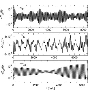
Figure 1: The fluctuations in the isoscalar axial quadrupole moment as a function of time are shown for ¹⁶O, ³²S, and ⁴⁰Ca using the SkM^∗ interaction. The size of the time step is $0.4$ fm/c. A grid of $24^{3}$ with a Cartesian box dimensioned $(-12,+12~{}{\rm fm})^{3}$ is used.

From the numerical solution of the TDHF equations, we obtain the density fluctuation as a function of time, Eq. (12). After Fourier transforming this quantity and folding with the function $F(\bm{x})$, we obtain $f(\omega)S(\omega)$ in Eq. (15), from which the linear response structure function of the system is extracted.

III Numerical Details and Results

The static and time-dependent Hartree-Fock calculations are performed using a collocation spline basis in a three-dimensional lattice configuration. Basis-Splines allow for the use of a lattice grid representation of the nucleus, which is much easier to use than alternate basis techniques, such as multi-dimensional harmonic oscillators. Also, for studies of exotic nuclei, because of weak binding, the density distributions tend to extend to large distances and hence one finds a large sensitivity to a harmonic oscillator basis due to the unphysical description of continuum states, while for a lattice grid representation one needs to simply increase the size of the box. Traditional grid representations typically use finite difference techniques to represent the gradient operator. Collocation Basis-Splines allow for the gradient operator to be represented by its action upon a basis function in a matrix form. Thus the collocation method gives a much more accurate representation of the gradient, while maintaining the convenience of a lattice grid and hence provides a much more accurate calculation in the end umar4 .

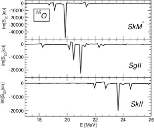
Figure 2: The imaginary part of the response function corresponding to the isoscalar quadrupole moment is shown for ¹⁶O using three different Skyrme force parametrizations, where the SkM^∗, SgII and SkII versions are shown in the upper, middle and lower panels, respectively. The experimentally measured giant quadrupole resonance is around 20.7 MeV.

We have performed the usual tests for assuring convergence with respect to the numerical box size and the number of collocation points. Typically a 7th order B-spline is used in a $(12~{}{\rm fm})^{3}$ box with $20^{3}-24^{3}$ grid points. The calculation can be performed with or without assuming time-reversal symmetry. The collective linear response may involve particle-hole interactions which are spin-dependent and not time-reversal symmetric. Therefore, for the correct collective content to be included one should not impose time-reversal symmetry in the linear response calculations krewald . In the results presented in this paper time-reversal symmetry is not imposed. In a comparison it is found that imposing time-reversal symmetry causes small shifts in the position of the collective modes on the order of $\approx 0.3$ MeV.

Calculations of isovector dipole; isovector and isoscalar octupole; and isoscalar quadrupole collective modes are performed for ¹⁶O, ³²S, and ⁴⁰Ca using several parameterizations of the Skyrme interaction. Here the parameterizations known as SkII SkII , SkM^∗ skm and SgII SgII are used for comparisons. The exponent of the density in the density-dependent term in SkII is $\alpha=1$, while for SkM^∗ and SgII this exponent is $\alpha=\frac{1}{6}$. This causes the SkII force to produce a rather large nuclear matter incompressibility, while the SkM^∗ and SgII forces produce more realistic compression properties. Also the SkM^∗ and SgII forces allow for more stable static Hartree-Fock and TDHF computations. The static Hartree-Fock calculations converge more easily and rapidly for SkM^∗ and SgII than for SkI, SkII or SkIII. A time step of $\Delta t=0.4$ fm/c is used for the calculation. It is found that one can perform the time evolution for up to 32768 time steps without appreciable dissipation. The results shown here use 16384 time steps for a maximum time of $\approx 6550$ fm/c.

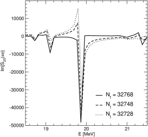
Figure 3: FFT results for ¹⁶O using three different numbers of time steps. The case when the number of time steps equals an exact power of two (32768) is clearly the better converged result, showing almost no positive values.

Reasonable results are obtained if the parameter $\varepsilon$ in Eq. (17) is chosen to fall in the range $2.0\times 10^{-4}\leq\varepsilon\leq 2\times 10^{-7}$. By varying the value of $\varepsilon$, the amplitude of the time-dependent density fluctuation then scales proportionally to $\varepsilon$, thus indicating that we are well within the linear regime of the theory.

The linear response calculations require well converged initial static HF solutions. To test for the convergence of the static HF calculation the energy fluctuation, which is the variance of $\widehat{H}$, is minimized. The energy fluctuation is defined as

$$\sqrt{\left|\langle{\widehat{H}}^{2}\rangle-\langle{\widehat{H}}\rangle^{2}\right|},$$ (20)

which measures how close the wave functions are to being eigenstates of $\widehat{H}$. This measure of convergence is very sensitive to the eigensolutions and is independent of the iteration step size. For ¹⁶O it was found that static HF solutions with energy fluctuation less than about $1.0\times 10^{-5}$ provided adequate starting points for the dynamic calculation, although the smaller the energy fluctuation the better.

The dynamic calculations involve using Eq. (II) to evolve the system. Since $U(t,t^{\prime})$ is an unitary operator, the orthonormality of the system is preserved, therefore it is not necessary to re-orthogonalize the solutions after every time-step. The stability of the calculation is checked by testing the preservation of the norm of each wave function. The number of terms in the expansion of the exponent in Eq. (II) is determined by requiring the norm to be preserved to a certain accuracy (typically to $\leq 1.0\times 10^{-8}-5.0\times 10^{-10}$).

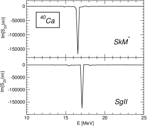
Figure 4: The imaginary part of the response function corresponding to the isoscalar quadrupole moment is shown for ⁴⁰Ca using two different Skyrme force parametrizations, SkM^∗ and SgII.

The time-dependent perturbing part of the Hamiltonian is evaluated when the exponential term in Eq. (17) is greater than some small number, $\varepsilon_{cut}$. Since it is not difficult to evaluate the action of the external part of the Hamiltonian on the wave function, $\varepsilon_{cut}$ is chosen to be very small, ($1.0\times 10^{-10}$). To allow the Fourier transform of $f(t)$ to be evaluated easily, it is necessary to integrate $t$ from $-\infty$ to $\infty$ and hence we would like the entire Gaussian of the perturbing function, $f(t)$, to be included into the time evolution to the desired accuracy. The parameter $t_{0}$ is therefore chosen such that the complete nonzero contribution of the time-dependent perturbation is included

$$t_{0}=-\left(2\Delta t+\sqrt{\left|\frac{2\log{\varepsilon_{cut}}}{\alpha}\right|}\right)\;.$$ (21)

III.1 Quadrupole Excitation Modes

For the study of the isoscalar quadrupole moment, the perturbing function $F(\bm{x})$, introduced in Eq. (3), is chosen to be the mass quadrupole moment, $Q_{20}=2z^{2}-(x^{2}+y^{2})$. It turns out that other even multipole modes are also excited at the same time (i.e. $Q_{40}$, $Q_{60}$, …). One can therefore study the effect of the coupling between the different excitation modes. The same holds true for the odd multipoles. This is due to the nonlinear response effects present in the TDHF time evolution SC03 .

The quadrupole collective resonances are calculated for ¹⁶O using three different Skyrme force parameterizations for comparisons. Two different size grids ($22^{3},24^{3}$) were used inside a ($-12,+12$ fm)³ Cartesian box along with periodic boundary conditions.

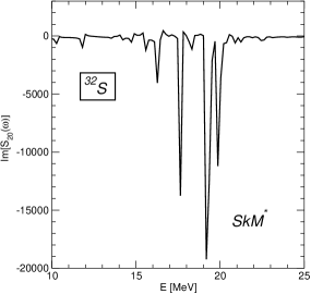
Figure 5: The imaginary part of the response function corresponding to the isoscalar quadrupole moment is shown for ³²S using the SkM^∗ force.

In Fig. 1 the time-dependent evolution of the multipole moment defined as:

$$\langle{\widehat{Q}}_{20}(t)\rangle=\int d^{3}x\delta\langle{\widehat{n}}(\bm{x},t)\rangle Q_{20}(\bm{x})\;,$$ (22)

is shown for ¹⁶O, ³²S, and ⁴⁰Ca using the SkM^∗ interaction. This figure illustrates the periodic character of the calculations with almost no damping. In this case the smallest oscillation is about $65$ fm/c.

A fast Fourier transform (FFT) is used to calculate the Fourier transform of $\langle{\widehat{Q}}_{20}(t)\rangle$ to give $\langle{\widehat{Q}}_{20}(\omega)\rangle=f(\omega)S_{20}(\omega)$. The time-dependent perturbation function, $f(\omega)$ can then be easily factored out using Eq. (15). One can use the analytic expression for $f(\omega)$ or use a numerical FFT calculation, where the difference between the two methods ends up being negligible.

In Fig. 2 the quadrupole responses for ¹⁶O are shown for the three different Skyrme cases. The imaginary part of Eq. (22) is Fourier transformed and divided by $f(\omega)$. Recalling Eq. (16), this quantity is derived to be a negative definite quantity. The SkM^∗ results for ¹⁶O reflect this property very well in Fig. 2. We observe a sharp peak at about $20$ MeV and a response which is almost purely negative. The side peaks, which are much less prominent, may not represent physical effects, but may be due to the construction of the continuum. In performing FFT transformations we find it to be important to have the number of points to be a power of two. In Fig. 3 we demonstrate this by plotting the response function for three different choices for the total number of time steps which differ from each other by only 20 points each. As one can see the case for 32768 points results in almost no positive values, indicating good convergence. The three cases give similar pole structures, which are near the experimental isoscalar quadrupole giant resonance. The experimental peak is centered at an energy of $20.7$ MeV with a width of about $7.5\pm 1$ MeV data . The resonance calculated with the SgII Skyrme parametrization is closest to the experimental result, although SkM^∗ is also fairly close. The SkII parametrization poorly represents the data, but this force is known to give a bad representation of the collective nuclear properties. However, for the SkII parametrization we were able to compare our results for ¹⁶O to the continuum RPA calculations of krewald . We find that the difference between the two calculations is less than 2% for the L=2, 3, and 4 modes. The difference may be due to the omission of the spin-orbit term in the continuum RPA calculations. We find the closest agreement for the hexadecupole mode, where both calculations give a peak energy of 28.2 MeV. The widths of resonances are not accurately reproduced, because the continuum is included into the calculation in an approximate fashion and higher order correlations are missing in the TDHF approach. Since the calculations are performed in a box, the continuum is represented in terms of discrete pseudo-continuum states, whose density is sensitive to the size of the box. A larger box size is expected to better represent the continuum with a higher density of pseudo-continuum states.

The property represented in Eq. (16) of being purely negative is not strictly reflected by the SgII nor the SkII results. One can see that this property is approximately reflected, but it is clear the convergence of the solution for these two cases is not nearly as good as for the SkM^∗ case.

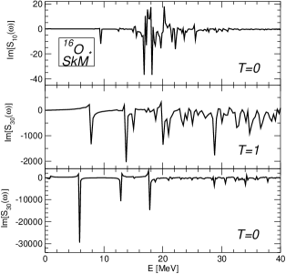
Figure 6: The imaginary part of the response function corresponding to the isoscalar and isovector octupole, and isovector dipole are shown for ¹⁶O using the SkM^∗ force.

An alternate check of the calculation is the energy-weighted sum rule (EWSR). This provides a stringent test of the normalization and is derivable from the static Hamiltonian. The SkM^∗ result gives $92\%$ of the EWSR, indicating excellent convergence. For SgII and SkII the linear response results give $66\%$ and $36\%$ of the EWSR, respectively, indicating a lack of convergence for these results.

The result for the SgII calculation is particular puzzling, since it is expected that the SkM^∗ and SgII interactions should be similar in behavior. The violations of the two convergence tests may be due to coupling to other collective modes, or may be due to numerical inconsistencies. We have investigated the SgII result by varying the size of the box, while keeping the grid spacing the same. We have found that a slightly larger box, (-14,+14) fm, seems to be closer to being purely negative.

In Fig. 4 we show the quadrupole strength function for ⁴⁰Ca using two different Skyrme parameterizations. In this case SkM^∗ and SgII show a peak at about 17 MeV. We also note the strength of the peak. In this case the resonance consumes all of the EWSR. In Fig. 5 we show the same quantity for ³²S using the Skyrme M^∗ force. In this case we observe multiple structures in the giant quadrupole resonance; the energy splitting arises from the prolate quadrupole deformation of the nuclear ground state in this system.

The resonant structure of the hexadecupole moment, $Q_{40}$, can also be calculated at the same time as the quadrupole moment. This corresponds to the coupling between the quadrupole and the hexadecupole collective modes. In this case if one were to include both $Q_{20}$ and $Q_{40}$ into the external time-perturbing piece of the total Hamiltonian, then this result corresponds to the coupling term:

$$f(\omega)S(\omega)=\frac{1}{\hbar}\int d^{3}x\int d^{3}x^{\prime}F^{\dagger}_{1}(\bm{x})D^{R}(\bm{x},\bm{x}^{\prime};\omega)F_{2}(\bm{x}^{\prime})f(\omega).$$ (23)

Here $F_{1}(\bm{x})\equiv Q_{40}(\bm{x})$ and $F_{2}(\bm{x}^{\prime})\equiv Q_{20}(\bm{x}^{\prime})$. For the pure hexadecupole giant resonance both $F_{1}$ and $F_{2}$ must be made equal to $Q_{40}$. In general, mixed mode analysis produces strength functions with less pronounced peaks and can be used when computational time saving is necessary.

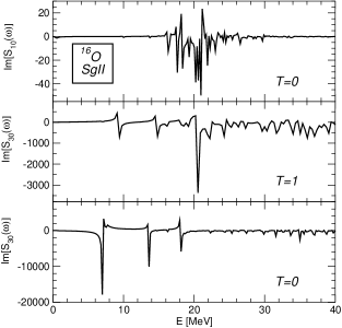
Figure 7: The imaginary part of the response function corresponding to the isoscalar and isovector octupole, and isovector dipole are shown for ¹⁶O using the SgII force.

III.2 Octupole and Dipole Modes

The octupole and dipole giant resonances are not symmetric about the $z=0$ plane and hence these nodes do not couple with the symmetric quadrupole and hexadecupole modes. The isovector octupole moment is defined as:

$$Q_{30}=\frac{1}{2}\left(1+\tau_{(3)}\right)\left[z^{3}-\frac{3}{2}z\left(x^{2}+y^{2}\right)\right].$$ (24)

In Fig. 6 the isoscalar dipole, isovector octupole, and isoscalar octupole responses are shown for ¹⁶O using the SkM^∗ interaction. In Fig. 7 the same quantities are again plotted using the SgII force. The isoscalar octupole mode shows three sharp resonance structures at about $6-7$ MeV, $13-14$ MeV, and $18$ MeV, for the SkM^∗ force, whereas the SgII resonances are at the slightly higher energies. These three peaks are also found in a spherical RPA calculation using the same effective interactions PG92 . The spherical calculation finds an additional broad peak for SkM^∗ and SgII centered at an energy of about $27-28$ MeV. This peak is weaker than the 3 peaks at lower energies and is not observed in the three-dimensional linear response calculation. In Fig. 6 one can see that the response is approximately purely negative, but that there are some violations of this feature.

The isovector octupole response is less clear than the other collective modes. It is also possible that resonances seen in the isoscalar octupole response may also appear in the isovector response due to couplings. In this case the strength of the peak is expected to be most prominent in its primary channel. This is most easily observed in Fig. 7 for the SgII force. In this case the lowest resonances at about $8-9$ MeV and at $14$ MeV are very close to the lowest peaks in the isoscalar case but with substantially reduced strength, whereas the most prominent isovector peak is at about $20$ MeV. The sorting of the isoscalar versus isovector mode is more complicated for the SkM^∗ force.

The isovector dipole response resulting from the linear response calculations is not as prominent as the isoscalar responses. This is most likely due to the absence of a strong collective dipole resonance for this nucleus. For the SkM^∗ case, there are some peaks centered around $17-18$ MeV, while for SgII the peaks range about $18-21$ MeV.

IV Summary and Conclusions

A method for evaluating the linear response theory using TDHF is formally developed and implemented. This method allows one to construct the dynamic calculation directly on top of the static Hartree-Fock calculation. Therefore, by performing a sophisticated and accurate three dimensional static Hartree-Fock calculation, we have a correspondingly accurate and consistent dynamic calculation. A coherent description of static ground state properties, such as binding energies and deformations is given along with a description of the collective modes of nuclei.

A three-dimensional collocation Basis-Spline lattice representation is used, which allows for a much more accurate representation of the gradient operator and hence a correspondingly accurate overall calculation. Example calculations of two spherical systems (¹⁶O, ⁴⁰Ca) and of a system with prolate quadrupole deformation (³²S) are presented for the response functions corresponding to various isoscalar and isovector multipole moments. The SkM^∗ case for the axial isoscalar quadrupole mode gives excellent results, obeying expectations from the theory and also satisfying the energy weighted sum rule.

- (1) G. F. Bertsch and S. F. Tsai, Phys. Reports 18, 125 (1975).
- (2) S. Krewald, V. Klemt, J. Speth, and A. Faessler, Nucl. Phys. A281, 166 (1977).
- (3) K. F. Liu and G. E. Brown, Nucl. Phys. A265, 385 (1976).
- (4) N. Van Giai and H. Sagawa, Nucl. Phys. A371, 1 (1981).
- (5) J. Blocki and H. Flocard, Phys. Lett. 85B, 163 (1979).
- (6) A. S. Umar, M. R. Strayer, R. Y. Cusson, P.-G. Reinhard, and D. A. Bromley, Phys. Rev. C 32, 172 (1985).
- (7) A.S. Umar and M.R. Strayer, Phys. Lett. 171B, 353 (1986).
- (8) C. Simenel, Ph. Chomaz, and G. de France, Phys. Rev. Lett. 86, 2971 (2001).
- (9) C. Simenel and Ph. Chomaz, Phys. Rev. C 68, 024302-1 (2003).
- (10) F.V. De Blasio, W. Cassing, M. Tohyama, P.F. Bortignon, and R.A. Broglia, Phys. Rev. Lett. 68, 1663 (1992).
- (11) M. Tohyama and A.S. Umar, Phys. Lett. B 549, 72 (2002).
- (12) O. Sorlin el. al, Phys. Rev. C 47, 2941 (1993).
- (13) A. S. Umar, J. Wu, M. R. Strayer and C. Bottcher, J. of Comp. Phys. 93, 426 (1991).
- (14) A. S. Umar, M. R. Strayer, J.-S. Wu, D. J. Dean and M. C. Güçlü, Phys. Rev. C 44, 2512 (1991).
- (15) A. L. Fetter and J. D. Walecka, Quantum Theory of Many-Particle Systems, (St. Louis: McGraw-Hill Book Co., 1971).
- (16) D. Vautherin and D. M. Brink, Phys. Rev. C 5, 626 (1972).
- (17) J. Bartel, P. Quentin, M. Brack, C. Guet, and H. B. Hankansson, Nucl. Phys. A 386, 79 (1982).
- (18) K. T. Knöpfle, G. J. Wagner, H. Breuer, M. Rogge, C. Mayer-Böricke, Phys. Rev. Lett. 35, 779 (1975).
- (19) P.-G. Reinhard and Y. Gambhir, Ann. Phys. (Leipzig) 1, 598 (1992); and private communication.