Analysis of Low-Momentum Correlations with Cartesian Harmonics

Abstract

Exploiting final-state interactions and/or identity interference, analysis of anisotropic correlations of particles at low-relative velocities yields information on the anisotropy of emission sources in heavy-ion reactions. We show that the use of cartesian surface-spherical harmonics in such analysis allows for a systematic expansion of the correlations in terms of real angular-moment coefficients dependent on relative momentum. The coefficients are directly related to the analogous coefficients for emission sources. We illustrate the analysis with an example of correlations generated by classical Coulomb interaction.

Correlations of particles at low relative velocities are commonly used for assessing geometric features of emission zones in nuclear reactions with multiparticle final states [1, 2]. At low relative momentum, the correlations exhibit structures, due to final-state interactions and/or identity interference, that are more pronounced for tighter emission zones. When particle emission zones are deformed, corresponding shape anisotropies are observed in the correlation function which can be studied as a function of the orientation of the relative momentum. Measured anisotropies in the correlation functions thus provide insight into the shape of the emission zone which is intimately connected to such aspects of the emission as reaction geometry, collective expansion, emission duration and differences in emission times for different species [3, 4, 5].

Final-state interactions and identity interference link the measured correlation function, ${\mathcal{R}}_{\bf P}({\bf q})$ (or alternatively ${\mathcal{C}}_{\bf P}({\bf q})$), to the source function, ${\mathcal{S}}_{\bf P}({\bf r})$, which provides the probability that two particles of the same velocity, whose total momentum is ${\bf P}$, are separated by a distance ${\bf r}$ at emission [6, 7]:

$${\mathcal{R}}_{\bf P}({\bf q})\equiv{\mathcal{C}}_{\bf P}({\bf q})-1\equiv\frac{\frac{{\rm d}^{6}N^{ab}}{{\rm d}^{3}p_{a}\,{\rm d}^{3}p_{b}}}{\frac{{\rm d}N^{a}}{{\rm d}^{3}p_{a}}\,\frac{{\rm d}N^{b}}{{\rm d}^{3}p_{b}}}-1=\int{\rm d}^{3}r\,\left[|\phi_{\bf q}^{(-)}({\bf r})|^{2}-1\right]\,{\mathcal{S}}^{ab}_{\bf P}({\bf r})\,.$$ (1)

Here, ${\bf q}$ and ${\bf r}$ are the relative momentum and relative spatial separation as determined by an observer in the two-particle rest frame and $\phi^{(-)}$ is the relative wave function for the asymptotic momentum ${\bf q}$. For particles with intrinsic spins, the square $|\phi^{(-)}|^{2}$ is averaged over spins, ensuring its dependence only on $q$, $r$ and the angle between the vectors, $\theta_{{\bf q}\,{\bf r}}$.

Various means have been employed to analyze anisotropies in correlations to provide quantitative measurement of the anisotropies in a source function. When analyzing identical pion correlations, the most common means has been to present projections of the correlation function along fixed directions of the relative momentum while constraining the remaining momentum components. Such projections often neglect regions of the data outside of the employed cuts and they can be clumsy if one is unaware of the best directions to orient the coordinate system. A second means for analyzing anisotropies involves fitting to three-dimensional parameterizations, such as for gaussian or blast-wave models [8]. Since source parameterizations typically employ on the order of 10 parameters, it can be difficult to determine the confidence of the fits due to the inherent complexity of cross correlations.

A third class of approaches involves applying tesseral spherical harmonics $Y_{\ell m}$ (regarding terminology for harmonics see [9]), to express the directional information in the correlation function and in the source function [10],

$${\mathcal{R}}_{\ell m}(q) = (4\pi)^{-1/2}\int{\rm d}\Omega_{\bf q}\,Y_{\ell m}^{*}(\Omega_{\bf q})\,{\mathcal{R}}({\bf q})\,,$$

$${\mathcal{S}}_{\ell m}(r) = (4\pi)^{-1/2}\int{\rm d}\Omega_{\bf r}\,Y_{\ell m}^{*}(\Omega_{\bf r})\,{\mathcal{S}}({\bf r}).$$ (2)

Here, the labels indicating the total momentum ${\bf P}$ and the particle types are suppressed. In terms of the projections, Eq. (1) can be re-expressed [10] as

$${\mathcal{R}}_{\ell m}(q)=4\pi\int{\rm d}r\,r^{2}\,K_{\ell}(q,r)\,{\mathcal{S}}_{\ell m}(r)\,,$$ (3)

where

$$K_{\ell}(q,r)=\frac{1}{2}\int{\rm d}\cos\theta_{\bf qr}\,P_{\ell}(\cos\theta_{\bf qr})\,\left[|\phi^{(-)}(q,r,\cos\theta_{\bf qr})|^{2}-1\right]\,.$$ (4)

Since a given $\ell m$ projection of ${\mathcal{R}}$ is only related to the same $\ell m$ projection of ${\mathcal{S}}$, the complexity of deconvoluting the shape information present in ${\mathcal{R}}$ is enormously simplified.

The disadvantage of expansion in the tesseral harmonics $Y_{\ell m}$ is that the connection between the geometric features of the real source function ${\mathcal{S}}({\bf r})$ and the complex valued projections ${\mathcal{S}}_{\ell m}(r)$ is not transparent. The $Y_{\ell m}$ harmonics are convenient for analyzing quantum angular momentum, but are clumsy for expressing anisotropies of real-valued functions. To rectify the shortcoming we propose performing a similar analysis using real-valued cartesian surface-spherical harmonics [11, 9] that directly address moments of the analyzed anisotropic functions. Cartesian harmonics are based on the products of unit vector components, $n_{\alpha_{1}}\,n_{\alpha_{2}}\cdots n_{\alpha_{\ell}}$. Due to the normalization identity $n_{x}^{2}+n_{y}^{2}+n_{z}^{2}=1$, at a given $\ell\geq 2$, the different component products are not linearly independent as functions of spherical angle; at a given $\ell$, the products are spanned by tesseral harmonics of rank $\ell^{\prime}\leq\ell$, with $\ell^{\prime}$ of the same evenness as $\ell$. Projecting away the lower-rank tesseral components, $\ell^{\prime}<\ell$, is a linear operation in the cartesian rank-$\ell$ space, represented by a rank-$2\ell$ tensor ${\mathcal{P}}^{(2\ell)}$ that produces cartesian rank-$\ell$ harmonics ${\mathcal{A}}^{(\ell)}_{\alpha_{1}\cdots\alpha_{\ell}}(\Omega)$:

$${\mathcal{A}}_{\alpha_{1}\cdots\alpha_{\ell}}^{(\ell)}=\sum_{\alpha_{1}^{\prime}\ldots\alpha_{\ell}^{\prime}}{\mathcal{P}}^{(2\ell)}_{\alpha_{1}\ldots\alpha_{\ell},\alpha_{1}^{\prime}\ldots\alpha_{\ell}^{\prime}}\,n_{\alpha_{1}^{\prime}}\cdots n_{\alpha_{\ell}^{\prime}}\,.$$ (5)

Tesseral harmonics of rank $\ell$, are, conversely, expressible in terms of the powers of unit-vector components of the order $\ell^{\prime}\leq\ell$, with $\ell^{\prime}$ of the same evenness as $\ell$. In the end, the harmonic ${\mathcal{A}}^{(\ell)}$ from (5) may be expressed as a combination of the powers of $n_{\alpha}$ of order $\ell^{\prime}\leq\ell$, where $\ell^{\prime}$ is of the same evenness as $\ell$, as shown in Table 1. The leading term is a simple product of unit vectors with the same indices as ${\mathcal{A}}$. Since cartesian harmonics ${\mathcal{A}}^{(\ell)}$ are linear combinations of tesseral harmonics of rank $\ell$, the product $r^{\ell}\,{\mathcal{A}}^{(\ell)}$ satisfies the Laplace equation.

Table 1: Cartesian surface-spherical harmonics of rank $\ell\leq 4$. Other harmonics can be found by permuting indices or switching indices, i.e., $x\leftrightarrow y$, $x\leftrightarrow z$ or $y\leftrightarrow z$.

${\mathcal{A}}^{(1)}_{x}=n_{x}$	${\mathcal{A}}^{(3)}_{xyz}=n_{x}\,n_{y}\,n_{z}$
${\mathcal{A}}^{(2)}_{xx}=n_{x}^{2}-1/3$	$A^{(4)}_{xxxx}=n_{x}^{4}-(6/7)n_{x}^{2}+3/35$
${\mathcal{A}}^{(2)}_{xy}=n_{x}\,n_{y}$	${\mathcal{A}}^{(4)}_{xxxy}=n_{x}^{3}\,n_{y}-(3/7)n_{x}\,n_{y}$
$A^{(3)}_{xxx}=n_{x}^{3}-(3/5)n_{x}$	${\mathcal{A}}^{(4)}_{xxyy}=n_{x}^{2}\,n_{y}^{2}-(1/7)n_{x}^{2}-(1/7)n_{y}^{2}+1/35$
${\mathcal{A}}^{(3)}_{xxy}=n_{x}^{2}\,n_{y}-(1/5)n_{y}$	${\mathcal{A}}^{(4)}_{xxyz}=n_{x}^{2}\,n_{y}\,n_{z}-(1/7)n_{y}\,n_{z}$

Because ${\mathcal{A}}^{(\ell)}$ is a linear combination of the tesseral harmonics of rank $\ell$, and because the kernel in Eq. (3) depends only on $\ell$ (and not $m$), an analogous equation to (3) can be derived for cartesian harmonic coefficients:

$${\mathcal{R}}^{(\ell)}_{\alpha_{1}\cdots\alpha_{\ell}}(q)=4\pi\int{\rm d}r\,r^{2}\,K_{\ell}(q,r)\,{\mathcal{S}}^{(\ell)}_{\alpha_{1}\cdots\alpha_{\ell}}(r)\,,$$ (6)

where the coefficients are defined as

$${\mathcal{R}}^{(\ell)}_{\alpha_{1}\ldots\alpha_{\ell}}(q) = \frac{(2\ell+1)!!}{\ell!}\int\frac{{\rm d}\Omega_{\bf q}}{4\pi}\,{\mathcal{A}}^{(\ell)}_{\alpha_{1}\ldots\alpha_{\ell}}(\Omega_{\bf q)}\,{\mathcal{R}}({\bf q})\,,$$

$${\mathcal{S}}^{(\ell)}_{\alpha_{1}\ldots\alpha_{\ell}}(r) = \frac{(2\ell+1)!!}{\ell!}\int\frac{{\rm d}\Omega_{\bf r}}{4\pi}\,{\mathcal{A}}^{(\ell)}_{\alpha_{1}\ldots\alpha_{\ell}}(\Omega_{\bf r})\,{\mathcal{S}}({\bf r})\,.$$ (7)

Cartesian harmonics satisfy the completeness relations:

$$\delta(\Omega^{\prime}-\Omega) = \frac{1}{4\pi}\sum_{\ell}\frac{(2\ell+1)!!}{\ell!}\sum_{\alpha_{1}\ldots\alpha_{\ell}}{\mathcal{A}}_{\alpha_{1}\ldots\alpha_{\ell}}^{(\ell)}(\Omega^{\prime})\,{\mathcal{A}}_{\alpha_{1}\ldots\alpha_{\ell}}^{(\ell)}(\Omega)$$ (8)

$$= \frac{1}{4\pi}\sum_{\ell}\frac{(2\ell+1)!!}{\ell!}\sum_{\alpha_{1}\ldots\alpha_{\ell}}{\mathcal{A}}^{(\ell)}_{\alpha_{1}\ldots\alpha_{\ell}}(\Omega^{\prime})\,n_{\alpha_{1}}\cdots n_{\alpha_{\ell}}\,.$$

Replacing ${\mathcal{A}}^{(\ell)}(\Omega)$ with the product $n_{\alpha_{1}}\cdots n_{\alpha_{\ell}}$ was justified by the fact that the projection operator is employed in ${\mathcal{A}}^{(\ell)}(\Omega^{\prime})$. Equation (8) allows one to restore ${\mathcal{R}}({\bf q})$ and ${\mathcal{S}}({\bf r})$ from the cartesian coefficients,

$${\mathcal{R}}({\bf q}) = \sum_{\ell}\sum_{\alpha_{1}\ldots\alpha_{\ell}}{\mathcal{R}}_{\alpha_{1}\ldots\alpha_{\ell}}^{(\ell)}\,\hat{q}_{\alpha_{1}}\cdots\hat{q}_{\alpha_{\ell}}\,,$$

$${\mathcal{S}}({\bf r}) = \sum_{\ell}\sum_{\alpha_{1}\ldots\alpha_{\ell}}{\mathcal{S}}_{\alpha_{1}\ldots\alpha_{\ell}}^{(\ell)}\,\hat{r}_{\alpha_{1}}\cdots\hat{r}_{\alpha_{\ell}}\,,$$ (9)

where $\hat{\bf q}$ and $\hat{\bf r}$ are unit vectors in the directions of ${\bf q}$ and ${\bf r}$.

Cartesian harmonics have other important properties. They are symmetric and traceless, i.e., if one sums ${\mathcal{A}}^{(\ell)}_{\alpha_{1}\cdots\alpha_{\ell}}$ over any two equated indices, the result is zero. In fact, the projection operator ${\mathcal{P}}$ in Eq. (5) is also referred to as a de-tracing operator. Tracelessness ensures, on its own, that $r^{\ell}\,{\mathcal{A}}^{(\ell)}$ satisfies the Laplace equation. While the $z$ axis is singled out in the construction of tesseral harmonics, the axes are treated symmetrically in the construction of cartesian harmonics, and different components can be obtained from each other by interchanging the $x$, $y$ and $z$ axes. For instance, the expression for ${\mathcal{A}}_{yzz}^{(\ell=3)}$ can be found by replacing replacing $n_{x}$ with $n_{z}$ in the expression for ${\mathcal{A}}_{xxy}^{(\ell=3)}$ in Table 1. Cartesian harmonics can be also generated recursively, beginning with ${\mathcal{A}}^{(\ell=0)}=1$,

$${\mathcal{A}}_{\alpha_{1}\ldots\alpha_{\ell}}^{(\ell)}(\Omega) = \frac{1}{\ell}\sum_{i}n_{\alpha_{i}}\,{\mathcal{A}}_{\alpha_{1}\ldots\alpha_{i-1}\,\alpha_{i+1}\ldots\alpha_{\ell}}^{(\ell-1)}(\Omega)-\frac{2}{\ell(2\ell-1)}$$ (10)

$$\times\sum_{i<j}\sum_{\alpha}\delta_{\alpha_{i}\,\alpha_{j}}\,n_{\alpha}\,{\mathcal{A}}_{\alpha\,\alpha_{1}\ldots\alpha_{i-1}\,\alpha_{i+1}\ldots\alpha_{j-1}\,\alpha_{j+1}\ldots\alpha_{\ell}}^{(\ell-1)}(\Omega)\,.$$

The above recursion can be used to obtain the coefficients for expanding the cartesian harmonics in terms of unit vector components [9]. The strategy of recursion, carried out in the other direction, leads to the coefficients of expansion of the products in terms of harmonics:

$$n_{x}^{\ell_{x}}\,n_{y}^{\ell_{y}}\,n_{z}^{\ell_{z}} = \sum_{m_{\alpha}\leq\ell_{\alpha}/2}\chi_{m_{x}\,m_{y}\,m_{z}}^{\ell_{x}\,\ell_{y}\,\ell_{z}}\,{\mathcal{A}}_{[\ell_{x}-2m_{x},\ell_{y}-2m_{y},\ell_{z}-2m_{z}]}^{(\ell-2m)}\,,$$ (11)

$$\chi_{m_{x}\,m_{y}\,m_{z}}^{\ell_{x}\,\ell_{y}\,\ell_{z}} \equiv \frac{(2\ell-4m+1)!!}{2^{m}\,(2\ell-2m+1)!!}\,\prod_{\alpha=x,y,z}\frac{\ell_{\alpha}!}{m_{\alpha}!\,(\ell_{\alpha}-2m_{\alpha})!}\,.$$

Here, $(-1)!!=1$, $m=m_{x}+m_{y}+m_{z}$, $\ell=\ell_{x}+\ell_{y}+\ell_{z}$ and $[\ell_{x},\ell_{y},\ell_{z}]$ is any set of indices where $x$ occurs $\ell_{x}$ times, $y$ occurs $\ell_{y}$ times and $z$ occurs $\ell_{z}$ times.

The expansion (11) is useful for calculating moments of ${\mathcal{S}}({\bf r})$,

$$\int{\rm d}^{3}r\,x^{\ell_{x}}\,y^{\ell_{y}}\,z^{\ell_{z}}\,{\mathcal{S}}({\bf r})\left/\int{\rm d}^{3}r\,{\mathcal{S}}({\bf r})\right. = \sum_{m_{\alpha}\leq\ell_{\alpha}/2}\frac{(\ell-2m)!}{(2\ell-4m+1)!!}\,\chi_{m_{x},m_{y},m_{z}}^{\ell_{x},\ell_{y},\ell_{z}}$$ (12)

$$\times\int{\rm d}r\,r^{\ell+2}\,{\mathcal{S}}_{[\ell_{x}-2m_{x},\ell_{y}-2m_{y},\ell_{z}-2m_{z}]}^{(\ell-2m)}(r)\left/\int{\rm d}r\,r^{2}\,{\mathcal{S}}^{(0)}(r)\right.\,.$$

In expansion in terms of cartesian harmonics, reflection symmetries with respect to the coordinate axes manifest themselves explicitly. Thus, if e.g. the source function is symmetric under the $y\rightarrow-y$ transformation, all odd-$\ell_{y}$ coefficients of ${\mathcal{S}}$ vanish.

Since rank-$\ell$ cartesian harmonics are linear combinations of rank-$\ell$ tesseral harmonics, cartesian harmonics of different $\ell$ are orthogonal to one another. Within a given rank, though, there are $(\ell+1)(\ell+2)/2$ combinations of $[\ell_{x},\ell_{y},\ell_{z}]$, while only $(2\ell+1)$ components can be independent. As an independent set, one can choose the components characterized by $\ell_{\alpha}=0,1$, for a selected coordinate $\alpha$, and the remaining harmonics within the rank can be generated via the traceleness property. For example, given harmonics for $\ell_{x}=0,1$, the application of ${\mathcal{A}}_{[\ell_{x}+2,\ell_{y},\ell_{z}]}=-{\mathcal{A}}_{[\ell_{x},\ell_{y}+2,\ell_{z}]}-{\mathcal{A}}_{[\ell_{x},\ell_{y},\ell_{z}+2]}$ yields the other harmonics. As for scalar product values within a rank, they can be found in [9].

For weak physical anisotropies it is likely that only the few lowest terms of angular expansion can be ascribed to the correlation functions or the source. For $\ell\leq 2$, the results can be summarized in terms of amplitudes and direction vectors as a function of $q$ and $r$, as illustrated here with the case of ${\mathcal{R}}$:

$${\mathcal{R}}({\bf q})={\mathcal{R}}^{(0)}(q)+\sum_{\alpha}\,{\mathcal{R}}^{(1)}_{\alpha}(q)\,\hat{q}_{\alpha}+\sum_{\alpha_{1}\,\alpha_{2}}{\mathcal{R}}^{(2)}_{\alpha_{1}\alpha_{2}}(q)\,\hat{q}_{\alpha_{1}}\,\hat{q}_{\alpha_{2}}+\ldots\,.$$ (13)

The function ${\mathcal{R}}^{(0)}$ is the correlation averaged over angles. The ${\mathcal{R}}^{(1)}$ components describe the dipole anisotropy and can be summarized in terms of the direction ${\bf e}^{(1)}(q)$ and magnitude $R^{(1)}(q)$, ${\mathcal{R}}^{(1)}_{\alpha}(q)=R^{(1)}\,e^{(1)}_{\alpha}$. The ${\mathcal{R}}^{(2)}$ components describe the quadrupole anisotropy and can be summarized in terms of three orthogonal principal direction vectors $\{{\bf e}_{k}^{(2)}(q)\}_{k=1,2,3}$ and three distortions that sum up to zero due to tracelessness: ${\mathcal{R}}^{(2)}_{\alpha\beta}(q)=R_{1}^{(2)}\,e_{1\alpha}^{(2)}\,e_{1\beta}^{(2)}+R_{3}^{(2)}\,e_{3\alpha}^{(2)}\,e_{3\beta}^{(2)}-\left(R_{1}^{(2)}+R_{3}^{(2)}\right)\,e_{2\alpha}^{(2)}\,e_{2\beta}^{(2)}$. For higher-order distortions, the direction of maximal distortion ${\bf e}_{3}^{(\ell)}$ may be defined as one maximizing the $\ell$’th cartesian harmonic projected in the direction of ${\bf e}_{3}$: $\sum_{\alpha_{1}\ldots\alpha_{\ell}}{\mathcal{R}}_{\alpha_{1}\ldots\alpha_{\ell}}^{(\ell)}\,{\bf e}_{3\alpha_{1}}^{(\ell)}\cdots{\bf e}_{3\alpha_{\ell}}^{(\ell)}$. The condition of maximum implies $\sum_{\alpha_{1}\ldots\alpha_{\ell}}{\mathcal{R}}_{\alpha_{1}\,\alpha_{2}\ldots\alpha_{\ell}}^{(\ell)}\,e_{k\,\alpha_{1}}^{(\ell)}\,e_{3\,\alpha_{2}}^{(\ell)}\cdots e_{3\,\alpha_{n}}^{(\ell)}$ $=0$, where $k=1,2$ and ${\bf e}_{1}^{(\ell)}$ and ${\bf e}_{2}^{(\ell)}$ span the space of directions perpendicular to ${\bf e}_{3}^{(\ell)}$. The direction of ${\bf e}_{1}^{(\ell)}$ may be chosen to minimize the projection of ${\mathcal{R}}^{(\ell)}$ in the plane perpendicular to ${\bf e}_{3}^{(\ell)}$.

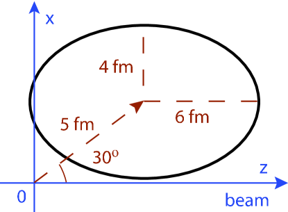
Figure 1: Characteristics of the sample source. The ellipse represents the contour of constant density within $x$-$z$ plane, at half the maximum density.

We next illustrate with an example how the correlation functions and source can be quantified following the cartesian coefficients. We choose a coordinate system with the $z$-axis along the beam direction and $x$-axis along the pair transverse momentum ${\bf P}^{\perp}$. We take a sample relative source for the particles, in a gaussian form with a larger 6 fm width in the beam direction and lower 4 fm widths in the transverse directions, cf. Fig. 1. The source is displaced from the origin by 5 fm, along ${\bf P}$ in system cm, assumed to point at 30^∘ relative to the beam axis. The cartesian coefficients are calculated for the source according to Eq. (9) and expressed in terms of amplitudes and angles shown in Figs. 2 and 3. The displayed dipole characteristics result then from: ${S}^{(1)}\,\sin{\theta_{S}^{(1)}}={\mathcal{S}}_{x}^{1}=3\int\frac{{\rm d}\Omega}{4\pi}\,{\mathcal{S}}({\bf r})\sin{\theta}$ and $S^{(1)}\,\cos{\theta_{S}^{(1)}}={\mathcal{S}}_{z}^{(1)}=3\int\frac{{\rm d}\Omega}{4\pi}\,{\mathcal{S}}({\bf r})\cos{\theta}$, and quadrupole from: ${\mathcal{S}}_{xx}^{(2)}=S_{1}^{(2)}\cos^{2}{\theta_{S}^{(2)}}+S_{3}^{(2)}\sin^{2}{\theta_{S}^{(2)}}$, ${\mathcal{S}}_{zz}^{(2)}=S_{1}^{(2)}\sin^{2}{\theta_{S}^{(2)}}+S_{3}^{(2)}\cos^{2}{\theta_{S}^{(2)}}$ and ${\mathcal{S}}_{xz}^{(2)}=\left(S_{3}^{(2)}-S_{1}^{(2)}\right)\sin^{2}{\theta_{S}^{(2)}}$, where ${\mathcal{S}}_{xx}^{(2)}=\frac{15}{2}\int\frac{{\rm d}\Omega}{4\pi}\,{\mathcal{S}}({\bf r})\left(\sin^{2}{\theta}\cos^{2}{\phi}-\frac{1}{3}\right)$, ${\mathcal{S}}_{zz}^{(2)}=\frac{15}{2}\int\frac{{\rm d}\Omega}{4\pi}\,{\mathcal{S}}({\bf r})\left(\cos^{2}{\theta}-\frac{1}{3}\right)$ and ${\mathcal{S}}_{xz}^{(2)}=\frac{15}{2}\int\frac{{\rm d}\Omega}{4\pi}\,{\mathcal{S}}({\bf r})\cos{\theta}\sin{\theta}\cos{\phi}$.

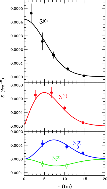
Figure 2: Low-$\ell$ values of the sample relative source, as a function of the relative distance $r$. Lines and symbols represent, respectively, exact values and values obtained through imaging of an anisotropic correlation function. Top panel shows the source averaged over angles, $S^{(0)}$. Middle panel shows the dipole distortion $S^{(1)}$. Bottom panel shows the larger, $S_{3}^{(2)}$, and smaller, $S_{1}^{(2)}$, quadrupole distortions within the $x$-$z$ plane.

Despite the fact that the maximum of source density ${\mathcal{S}}$ occurs away from ${\bf r}=0$, the angle-averaged source $S^{(0)}$ in Fig. 2 is maximal at $r=0$. An analytic source function ${\mathcal{S}}$ may be Taylor expanded in three dimensions about ${\bf r}=0$. The lowest-order terms of the Taylor expansion that can contribute to a rank-$\ell$ cartesian coefficient of ${\mathcal{S}}$ must involve an $\ell$’th order derivative and rise as $r^{\ell}$, as is apparent in Fig. 2. The subsequent contributing terms rise as $r^{\ell+2k}$, $k=1,2,\ldots$, which is important if one tries to parameterize the functions $S^{(\ell)}$.

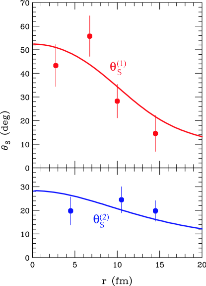
Figure 3: Angles characterizing the dipole (top) and quadrupole (bottom) distortions of the sample relative source, as a function of the relative distance $r$. Lines and symbols represent, respectively, exact angles and angles obtained from imaging of an anisotropic correlation function.

At low $r$, the angles $\theta_{S}^{(1)}$ and $\theta_{S}^{(2)}$ are determined by the derivatives of ${\mathcal{S}}$ at ${\bf r}=0$; in particular $\theta_{S}^{(1)}$ gives the direction of the gradient. At high $r$, the angles follow the elongation of the gaussian and, correspondingly, they approach zero as $r\rightarrow\infty$.

Next, we determine correlation function coefficients for our sample source, examine how the coefficients reflect the source features and attempt to restore those features through imaging. We choose the classical limit of repulsive Coulomb interactions for the emitted particles, such as appropriate for intermediate mass fragments [12, 13]. The kernel for Eqs. (1) and (4) can be analytically calculated by considering changes in momentum volume associated with Coulomb trajectories, $|\phi|^{2}={\rm d^{3}}\,q_{0}/{\rm d^{3}}\,q$, where ${\bf q}_{0}$ is the starting momentum at the separation ${\bf r}$. The result depends only on the angle $\theta_{{\bf q}{\bf r}}$ and on the separation at emission scaled with the distance of closest approach in a head-on collision, $r/r_{c}$, where $q^{2}/2m_{ab}=Z_{a}\,Z_{b}\,e^{2}/4\pi\epsilon_{0}\,r_{c}$:

$$|\phi^{(-)}(q,r,\cos\theta_{\bf qr})|^{2}=\frac{\Theta\left(1+\cos{\theta_{{\bf q}{\bf r}}}-{2r_{c}}/{r}\right)\,(1+\cos{\theta_{{\bf q}{\bf r}}}-{r_{c}}/{r})}{\sqrt{\left(1+\cos{\theta_{{\bf q}{\bf r}}}\right)^{2}-\left(1+\cos{\theta_{{\bf q}{\bf r}}}\right){2r_{c}}/{r}}}\,.$$ (14)

The $\ell=0$ kernel is $K_{0}=\Theta(r-r_{c})\,\sqrt{1-r_{c}/r}-1$, while the $K_{\ell\geq 1}$ components are, generally, calculated numerically from (4).

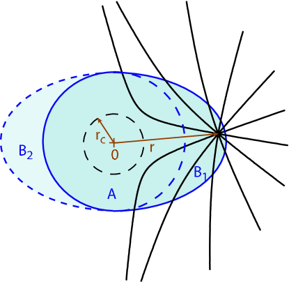
Figure 4: A schematic relative source with repulsive Coulomb trajectories superimposed coming out isotropically from position ${\bf r}$ within the source. The region of radius $r_{c}$ is inaccessible to the trajectories. The source consists of an isotropic part A, axially symmetric part B₁, responsible for source deformation, and, optionally, part B₂ that is a mirror reflection of B₁.

The Coulomb trajectories are illustrated in Fig. 4. The repulsive Coulomb force principally focuses the trajectories towards the direction of ${\bf r}$ they originate from. For $r_{c}\ll r$ (large $q$), the $K_{\ell}$ kernels from from (4) are affected by the deflection of trajectories away from $\cos{\theta_{\bf qr}}\sim-1$. With $P_{\ell}(\cos{\theta}\rightarrow-1)=(-1)^{\ell}$, the kernels in this limit are $K_{\ell}\simeq(-1)^{\ell}\,K_{0}\simeq(-1)^{\ell+1}\,r_{c}/2r$, with the additional negative sign representing trajectory depletion. For $r-r_{c}\ll r_{c}$ (low $q$), the kernels are affected by the trajectories bunching up around $\cos{\theta_{\bf qr}}\sim 1$. With $P_{\ell}(\cos{\theta}\rightarrow 1)=+1$, the kernels in this limit are $K_{\ell\geq 1}\simeq K_{0}+1=\Theta(r-r_{c})\,\sqrt{r/r_{c}-1}$. The $K_{1}$ kernel is always positive and, thus, the dipole distortion of the correlation generally points in the same direction as the distortion of the source, as for e.g. the source out of A and B₁ in Fig. 4. However, the $K_{2}$ kernel switches sign at $r/r_{c}=1.63$. At $r/r_{c}<1.63$, a prolate source, such as out of A and B₁ (and possibly B₂) in Fig. 4, results in a prolate correlation function elongated in the same direction. However, at $r/r_{c}>1.63$, the prolate source results in an oblate correlation with distortion pointing in transverse directions.

Figure 5 shows the characteristics of the correlation function ${\mathcal{C}}$, in terms of $\ell\leq 2$ cartesian coefficients, for the source of Fig. 1, as function of $r_{c}^{-1/2}\propto q$.

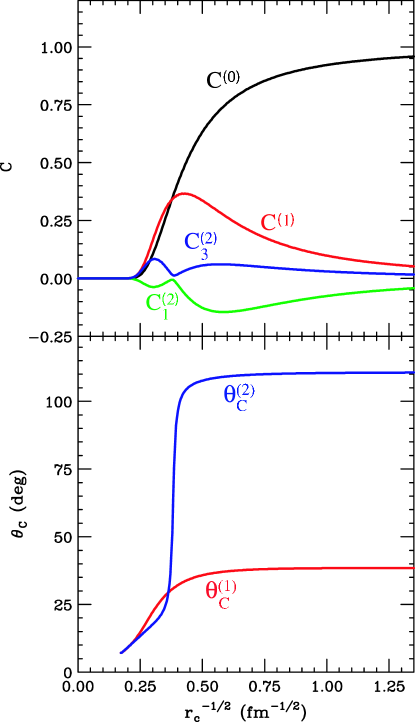
Figure 5: Low-$\ell$ characteristics of the Coulomb correlation function for our sample source: amplitudes (top panel) and angles (bottom panel) as a function of inverse square root of the head-on return radius $r_{c}$.

The dependence $\theta_{C}^{(1)}(r_{c})$ in Fig. 5 generally retraces the dependence $\theta_{S}^{(1)}(r)$ of Fig. 3, where $r_{c}\lesssim r$, as anticipated. However, while $\theta_{C}^{(2)}(r_{c})$ starts out in a similar fashion, it jumps by $90^{\circ}$ as $K_{2}$ switches sign, with $r$ in $r/r_{c}\sim 1.6$ characterizing the source quadrupole distortion. The jump is accompanied by the cross-over behavior for the distortions $C^{(2)}$, expected for the kernel sign change. In the low and high $q$ limits, the correlation coefficients approach universal integrals of source coefficients, such as ${\mathcal{R}}_{\alpha_{1}\ldots\alpha_{\ell}}^{(\ell)}(r_{c})={\mathcal{C}}^{(\ell)}_{\alpha_{1}\ldots\alpha_{\ell}}(r_{c})-\delta_{\ell 0}\simeq 2\pi r_{c}\,(-1)^{\ell+1}\int_{0}^{\infty}{\rm d}r\,r\,{\mathcal{S}}^{\ell}_{\alpha_{1}\ldots\alpha_{\ell}}(r)$, for $r_{c}\ll r$. In that limit, from $r_{c}^{-1/2}\sim 0.9\,\mbox{fm}^{-1/2}$ on in Fig. 5, the relative magnitudes of $(-1)^{\ell}\,R^{(\ell)}$ reflect the relative magnitudes of the $S^{(\ell)}$ distortions for the integrated traceless tensors.

We next illustrate imaging of source components from the correlation [10, 14, 15, 16, 17, 18]. The tensorial decomposition allows to use different source representations within subspaces of different tensorial rank. With a source coefficient represented in the basis $\{B_{i}\}$ as ${\mathcal{S}}(r)=\sum_{i}{\mathcal{S}}_{i}\,B_{i}(r)$, the ${\mathcal{R}}$ function at $j$’th discrete value of $q$ (or $r_{c}^{-1/2}$ in our case), is ${\mathcal{R}}_{j}=K_{ji}\,{\mathcal{S}}_{i}$. Here, following (6), the matrix elements are $K_{ji}=4\pi\int_{0}^{\infty}{\rm d}r\,r^{2}\,K(q_{j},r)\,B_{i}(r)$ and the spherical-tensor indices are suppressed. Minimization of $\chi^{2}=\sum_{j}({\mathcal{R}}_{j}-{\mathcal{R}}_{j}^{exp})^{2}/\sigma_{j}^{2}$ with respect to $\{S_{i}\}$ yields the result, in matrix form,

$${\mathcal{S}}=(K^{\top}\,\sigma_{\mathcal{C}}^{-2}\,K)^{-1}\,K^{\top}\,\sigma_{\mathcal{C}}^{-2}\,{\mathcal{R}}\,,$$ (15)

where $(\sigma_{\mathcal{C}}^{-2})_{jk}=\delta_{jk}/\sigma_{j}^{2}$. Equation (15) is the basis of imaging, i.e. determining ${\mathcal{S}}^{(\ell)}_{\alpha_{1}\cdots\alpha_{\ell}}$ values from ${\mathcal{R}}^{(\ell)}_{\alpha_{1}\cdots\alpha_{\ell}}$. For illustration, we assume that the $\ell\leq 2$ cartesian coefficients of the correlation function for our sample source have been measured at 80 values of $r_{c}^{-1/2}$, between 0 and $3\,\mbox{fm}^{-1/2}$, subject to an r.m.s. error of $\sigma=0.015$. For the basis $\{B_{i}\}$ we take take simple rectangle functions that, within basis splines, we generally find to provide the most faithful source values. As relative errors decrease with increasing multipolarity, we reduce the number of functions in restoration, from 5 for $\ell=0$ to 3 for $\ell=2$, all spanning the region $r<17\,\mbox{fm}$. Upon sampling the cartesian coefficients of ${\mathcal{R}}$, we restore the coefficients of ${\mathcal{S}}$ following (15) and obtain the results represented by symbols in Figs. 2 and 3 for central arguments of the basis functions. As is apparent, under realistic circumstances, angular features of the source can be quantitatively restored.

Having the imaged $\ell\leq 2$ source coefficients, we can calculate the $\ell\leq 2$ cartesian moments for the imaged region from (12). For the image we find, with statistical errors of restoration: $4\pi\int{\rm d}r\,r^{2}\,{\mathcal{S}}^{(0)}=0.99\pm 0.05$, $\langle x\rangle=(1/3)\int{\rm d}r\,r^{3}\,{\mathcal{S}}_{x}^{(1)}/\int{\rm d}r\,r^{2}\,{\mathcal{S}}^{(0)}=2.47\pm 0.11\,\mbox{fm}$, $\langle z\rangle=4.25\pm 0.13\,\mbox{fm}$, $\langle(x-\langle x\rangle)^{2}\rangle^{1/2}=3.80\pm 0.24\,\mbox{fm}$, $\langle y^{2}\rangle^{1/2}=3.81\pm 0.22\,\mbox{fm}$, $\langle(z-\langle z\rangle)^{2}\rangle^{1/2}=5.54\pm 0.19\,\mbox{fm}$ and $\langle(x-\langle x\rangle)(z-\langle z\rangle)\rangle=2.23\pm 1.49\,\mbox{fm}^{2}$, which can be compared to the $r<17\,\mbox{fm}$ results from the original source of, respectively: 1.00, 2.45 fm, 3.90 fm, 3.99 fm, 4.00 fm, 5.60 fm and $-0.41\,\mbox{fm}^{2}$.

In summary, we have discussed the utility of cartesian surface-spherical harmonics in the analysis of particle correlations at low relative-velocities. The cartesian harmonics allow for a systematic quantification of anisotropic correlation functions, through expansion coefficients related to analogous expansion coefficients for anisotropic emission sources. For illustrating the relation, we have employed correlations produced by classical Coulomb interactions. To an extent, the features of source anisotropies may be read off directly from the correlation anisotropies; otherwise, they can be imaged.

References

[1]
U. W. Heinz and B. V. Jacak, Ann. Rev. Nucl. Part. Sci. 49 (1999)
529.
[2]
W. Bauer, C. K. Gelbke and S. Pratt, Ann. Rev. Nucl. Part. Sci. 42
(1992) 77.
[3]
R. Lednicky, V. L. B. Erazmus and D. Nouais, Phys. Lett. B 373 (1996) 20.
[4]
S. Voloshin, R. Lednicky and S. Panitkin, Phys. Rev. Lett. 79
(1997) 4766.
[5]
C. J. Gelderloos et al., Phys. Rev. Lett. 75 (1995) 3082.
[6]
S. E. Koonin, Phys. Lett. B 70 (1977) 43.
[7]
D. Anchishkin, U. W. Heinz and P. Renk, Phys. Rev. C 57 (1998) 1428.
[8]
F. Retiere and M. A. Lisa,
Phys. Rev. C 70 (2004) 044907.
[9]
J. Applequist, Theor. Chem. Acc. 107 (2002) 103.
[10]
D. A. Brown and P. Danielewicz, Phys. Lett. B 398 (1997) 252.
[11]
J. Applequist, J. Phys. A: Math. Gen. 22 (1989) 4303.
[12]
Y. Kim, R. de Souza, C. Gelbke, W. Gong, and S. Pratt, Phys. Rev. C 45
(1992) 387.
[13]
S. Pratt and S. Petriconi, Phys. Rev. C 68 (2003) 054901.
[14]
D. A. Brown and P. Danielewicz, Phys. Rev. C 64 (2001) 014902.
[15]
S. Y. Panitkin et al., Phys. Rev. Lett. 87 (2001) 112304.
[16]
G. Verde et al., Phys. Rev. C 65 (2002) 054609.
[17]
G. Verde et al., Phys. Rev. C 67 (2003) 034606.
[18]
P. Chung et al., Phys. Rev. Lett. 91 (2003) 162301.