Density matrix renormalization group and wave function factorization for nuclei

Abstract

We employ the density matrix renormalization group (DMRG) and the wave function factorization method for the numerical solution of large-scale nuclear structure problems. The DMRG exhibits an improved convergence for problems with realistic interactions due to the implementation of the finite algorithm. The wave function factorization of $fpg$-shell nuclei yields rapidly converging approximations that are at the present frontier for large-scale shell-model calculations.

1 Introduction

The nuclear shell model with full configuration mixing is the adequate tool for a quantitative description of light- and medium-mass nuclei. In recent years, the no-core shell model has successfully been applied to investigate $p$-shell nuclei [1, 2], and full-space diagonalizations involving model spaces with up to one-billion Slater determinants are now possible for $sd$-shell and $pf$-shell nuclei within the traditional shell model [3, 4, 5]. Note that it took more than a decade to go from $sd$-shell nuclei to $pf$-shell nuclei, and progress was due to more sophisticated algorithms and an increase in computer power. The description of heavier nuclei or drip-line nuclei, however, is based on increasingly larger model spaces. For such nuclei, exact diagonalizations will be unavailable for the next years, and one has to introduce approximations.

Several authors have suggested truncations of the model space. In many of these methods, the selection of the relevant basis states is based on physical insights and arguments and is done “by hand” [6, 7, 8]. In other methods, the Hamiltonian itself selects the most important basis states. One example is the Monte Carlo shell model [9], where the huge Hilbert space is sampled stochastically, and only relevant basis states are kept. Another example is provided by the density matrix renormalization group (DMRG) [10, 11] and the wave function factorization [12], where the most important basis states are determined from a variational principle. It is the purpose of this article to describe recent progress with the latter two methods. We report on DMRG results for $sd$-shell and $pf$-shell nuclei, and use the wave function factorization to compute accurate approximations for low-lying states in $0f_{5/2}\,1p\,0g_{9/2}$ shell nuclei that are at the frontier of full space diagonalizations.

2 Density matrix renormalization group

During the last decade, the DMRG has become the method of choice to compute ground state properties for spin-chains. We refer the reader to the review [13] and briefly describe the main aspects of this method. In the one-dimensional spin systems, the lattice is divided into two parts (e.g. “left” and “right”), and the ground state energy is computed for a small number of lattice sites. The ground state can be expressed in terms of basis states $|l\rangle$ and $|r\rangle$ of the “left” and “right” part of the chain, respectively, as

$$|\Psi\rangle=\sum_{l,r=1}^{M}\Psi_{lr}|l\rangle|r\rangle.$$ (1)

In the DMRG, one seeks an approximation of $|\Psi\rangle$ in terms of $m<M$ basis states. These states are the eigenstates of the density matrices $\rho_{ll^{\prime}}=\sum_{r}\Psi_{lr}\Psi_{l^{\prime}r}$ and $\rho_{rr^{\prime}}=\sum_{l}\Psi_{lr}\Psi_{lr^{\prime}}$ that correspond to the $m$ largest eigenvalues. This is a truncation for which the difference between exact ground state and approximated ground state has minimal norm [11]. One then retains these $m$ states for the left and right part of the lattice, and adds another lattice site to either part. This procedure defines the “infinite algorithm” and is repeated until the desired system size is reached. At this point, an iterative procedure known as the “finite algorithm” is used to enlarge one part of the lattice at the expense of the other while keeping the total number of lattice sites constant. This defines a “sweep” through the system. Typically one finds that the truncation error decreases exponentially with the number $m$ of kept states. Note that one does not store the wave function in the DMRG. Instead, one keeps $m$-dimensional matrix representations of those operators that define the Hamiltonian and other observables of interest.

Only recently has the DMRG also been applied to finite Fermi systems, and we refer the reader to the recent review by Dukelsky and Pittel [14]. There are at least three novelties for the DMRG in finite Fermi systems. First, an order of lattice sites, i.e. single-particle orbitals has to be chosen. Second, a partition of the system in two parts has to be chosen. Third, the two-body interaction induces interactions between very distant single-particle orbitals and thereby differs from the spin chains with neighboring interactions. For nuclei, Dukelsky and coworkers suggest an ordering of the single-particle orbitals based on their distance from the Fermi surface and based the partition on particle versus hole orbitals [15]. Using the infinite DMRG algorithm, they obtained rapidly converging results for schematic pairing and pairing-plus-quadrupole models but encountered rather slow convergence for $sd$-shell nuclei with more realistic (and complex) interaction [16].

Our implementation of the DMRG is as follows. We choose a partition of neutron orbitals versus proton orbitals. This is motivated by our experience with the wave function factorization. The spherical single particle orbitals have quantum numbers $\alpha=(n,l,j,j_{z},\tau_{z})$. We work in the $m$ scheme and conserve total angular momentum $J_{z}$ at each step of the DMRG. As the equivalent of a single lattice site, we choose conjugate pairs $(\alpha,\bar{\alpha})$ of single-particle orbitals. This is designed to improve angular momentum properties and to properly treat pairing correlations. The conjugate pairs of single-particle orbitals are ordered such that the most active orbitals, i.e. the orbitals close to the Fermi surface are in the center of the chain of orbitals. This is motivated by the extensive studies reported by Legeza on this subject [17]. To overcome difficulties with the long-ranged two-body interaction, we use the finite algorithm. We do not use the infinite algorithm. Instead, we start the finite algorithm based on the spherical Hartree-Fock configuration and its $1p$-$1h$ excitations. We find that this approach is superior to the infinite algorithm and the approach suggested by Xiang for treating systems with conserved quantities [18]. Note that we also considered DMRG calculations in a Hartree-Fock basis. Compared to the DMRG in the spherical basis, this approach lowered the energy at the start of the finite algorithm. However, the breaking of axial symmetry led to larger-dimensional matrix problems and did not improve the convergence of the method. In the practical calculations, we start with the finite algorithm with a rather small number $m$ of kept states and increase this number every two sweeps.

We performed DMRG calculations for the $sd$-shell nucleus ²⁸Si using the USD interaction [19]. The order of the (pairs) of single-particle orbitals is $d_{3}3$, $d_{3}1$, $d_{5}5$, $d_{5}3$, $s_{1}1$, $d_{5}1$, $d_{5}1$, $s_{1}1$, $d_{5}3$, $d_{5}5$, $d_{3}1$, $d_{3}3$, where we used the notation $l_{2j}|2j_{z}|$, and it is understood that the first half of orbitals corresponds to proton states, while the (mirror symmetric) second half of orbitals corresponds to the neutron states. The initial set of states consists of the $(d_{5/2})^{12}$ configuration and its $1p$-$1h$ excitations. The left part of Fig. 1 shows the DMRG results for the ground state energy as a function of the number of states we keep. The energy converges exponentially rapidly as more states are kept, and the true ground state energy can accurately be determined from an exponential fit to the data. The inset shows the dimension of the DMRG eigenvalue problem as a function of the number of kept states. Note that the full eigenvalue problem has dimension $d=93710$.

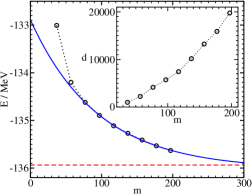
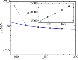
Figure 1: Left: DMRG ground state energies for ²⁸Si as a function of the number $m$ of kept states (data points connected by dots), exact result (dashed line), and exponential fit (full line). The inset shows the dimension $d$ of the DMRG eigenvalue problem vs. $m$. Right: Same as left except for ⁵⁶Ni.

This promising result motivates us to perform DMRG calculations for the $fp$-shell nucleus ⁵⁶Ni. We use the KB3 interaction [20, 21]. The exact diagonalization of this shell-model problem has to deal with about one billion Slater determinants and has only been accomplished recently [4]. The order of single-particle orbitals is $f_{5}5$, $f_{5}3$, $f_{5}1$, $p_{1}1$, $f_{7}7$, $f_{7}5$, $p_{3}3$, $f_{7}3$, $p_{3}1$, $f_{7}1$, $f_{7}1$, $p_{3}1$, $f_{7}3$, $p_{3}3$, $f_{7}5$, $f_{7}7$, $p_{1}1$, $f_{5}1$, $f_{5}3$, $f_{5}5$. The initial set of states consists of the $(f_{7/2})^{16}$ configuration and its $1p$-$1h$ excitations. The right part of Fig. 1 shows the results. The DMRG results seem to be converged as an increase of $m$ does not significantly lower the energy. However, the true ground state energy is almost 400 keV lower in energy. We recall that the structure of ⁵⁶Ni is to some extent similar to ²⁸Si. This similarity has motivated our choice of states to be kept at the beginning of the finite algorithm and our order of the single-particle orbitals. It is thus unexpected that the DMRG converges for ²⁸Si but fails to fully converge for the computationally larger problem ⁵⁶Ni.

Note however that our DMRG computations exhibit an improved convergence when compared to the pioneering study [16]. The most important new ingredients are the use of the finite algorithm, the abandoning of the infinite algorithm, and the ordering of the single-particle orbitals. We expect that further improvement of the convergence relies on an optimal order of single-particle orbitals and on optimal initial conditions for the finite algorithm. The method presented in the following section avoids these issues and makes use only of the unproblematic truncation step of the DMRG.

3 Wave function factorization

Modern shell model codes build their basis from products of Slater determinants $|\pi\rangle$ for the proton space and Slater determinants $|\nu\rangle$ for the neutron space. Note that the dimensions of the proton and neutron space are modest compared to the dimension of the product space. A shell-model ground state might thus be expanded as

$$|\Psi\rangle=\sum_{\pi,\nu}\Psi_{\pi\nu}|\pi\rangle|\nu\rangle,$$ (2)

where the sum runs over all available proton and neutron determinants. This expansion is similar to Eq. (1) used in the DMRG. The amplitude matrix $\Psi_{\pi\nu}$ is rectangular in general and can be factored as $\Psi=USV^{\dagger}$ by means of the singular value decomposition (SVD). Here, $U$ and $V$ are unitary matrices that operate on the proton space and the neutron space, respectively, and $S$ is zero except for nonnegative entries $s_{jj}\geq 0$ (the “singular values”) along its diagonal. The SVD thus yields correlated proton and neutron states

$$|\tilde{p}_{j}\rangle = \sum_{\pi}U_{\pi j}|\pi\rangle,$$ (3)

$$|\tilde{n}_{j}\rangle = \sum_{\pi}V_{\nu j}|\nu\rangle,$$ (4)

and the ground state becomes $|\Psi\rangle=\sum_{j}s_{j}|\tilde{p}_{j}\rangle|\tilde{n}_{j}\rangle$. Note that the DMRG is closely related to the SVD: $\Psi\Psi^{\dagger}=USS^{\dagger}U^{\dagger}$ and $\Psi^{\dagger}\Psi=VS^{\dagger}SV^{\dagger}$ are density matrices which are diagonalized by the matrices $U$ and $V$, respectively, and their eigenvalues are the squares of the singular values [11]. Note also that the SVD yields exponentially rapidly decreasing singular values for ground states obtained from realistic shell-model interactions [22]. This observation is interesting for two reasons. First, it shows that the DMRG truncation step also works for nuclei. Second, it provides the basis for a powerful approximation and basis state selection scheme. In the wave function factorization, we approximate the ground state as a sum over $\Omega$ products of correlated proton and neutron states

$$|\Psi\rangle=\sum_{j=1}^{\Omega}|p_{j}\rangle|n_{j}\rangle.$$ (5)

Note that the states $|p_{j}\rangle$ and $|n_{j}\rangle$ are not normalized. Variation of the energy yields the following set of eigenvalue equations that determine the states $|p_{j}\rangle$ and $|n_{j}\rangle$

$$\sum_{i=1}^{\Omega}\left(\langle n_{j}|\hat{H}|n_{i}\rangle-E\langle n_{j}|n_{i}\rangle\right)|p_{i}\rangle = 0,$$

$$\sum_{i=1}^{\Omega}\left(\langle p_{j}|\hat{H}|p_{i}\rangle-E\langle p_{j}|p_{i}\rangle\right)|n_{i}\rangle = 0.$$ (6)

These equations can be solved iteratively. One starts with a random set of orthogonal neutron states $|n_{j}\rangle$ and solves the first of the eigenvalue problems in Eq. (3) for those proton states that correspond to the lowest energy $E$. These are then inserted in the second eigenvalue problem in Eq. (3), which is solved for the neutron states corresponding to the lowest energy. This procedure is repeated until the energy $E$ converges. For even-even nuclei, convergence is typically reached in 5-10 iterations, while other nuclei require a somewhat larger number of iterations. The eigenvalue problems (3) have dimension $\Omega D_{p}$ and $\Omega D_{n}$ for the proton states and neutron states, respectively, where $D_{p}$ ($D_{n}$) denotes the dimension of the proton (neutron) space. Typically, one needs only a few hundred states $\Omega$ for more than 99% overlap with the exact ground state. Thus, $\Omega\ll D_{p},D_{n}$, and the factorization requires one to solve eigenvalue problems of small dimensions relative to the exact diagonalization which has a dimension that scales as $D_{p}D_{n}$. Note that the proton and neutron states that enter the eigenvalue problem (3) can be kept orthogonal, and this reduces the generalized eigenvalue problem to a standard eigenvalue problem. Note also that axial or rotational symmetry can be conserved within the ansatz (5). For details, we refer the reader to Ref. [22].

In earlier work, we applied the factorization to $sd$-shell nuclei and $fp$-shell nuclei and demonstrated its accuracy and capability by comparing with results from exact diagonalization. In this work we use the factorization and perform structure calculations for a few $A=76,78$ nuclei. The model space consists of the $0f_{5/2}\,1p\,0g_{9/2}$ orbitals, and the interaction is a monopole-corrected $G$-matrix [23], taking ${}^{56}_{28}$Ni₂₈ as a closed core. These problems are at the present frontier of nuclear structure calculations. We mention, for instance, the recently accomplished exact diagonalziation for double beta-decay studies in ⁷⁶Ge and ⁷⁶Se [24, 25], and the determination of the $T=1$ two-body matrix elements by fit [26].

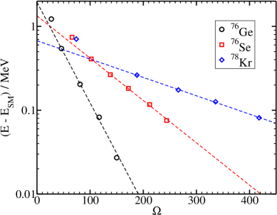
Figure 2: Data points: Ground state energies as a function of the number of retained states. Dashed lines: exponential fit to data.

In this article, we focus on the nuclei ⁷⁶Ge, ⁷⁶Se, and ⁷⁸Kr, and compute their lowest-lying states using the $m$-scheme factorization. For Se and Kr, we also use parity to reduce the dimensionality of the shell-model problem. Figure 2 shows the energy difference $E(\Omega)-E_{SM}$ of the ground states as a function of the number $\Omega$ of kept states. The shell-model energies $E_{SM}$ are determined by an exponential fit to the numerical data points and are listed in Table 1. Note that the wave function factorization uses a few hundred states out of up to several hundred thousand proton and neutron states. Deformed nuclei typically require more states as deformation is driven by proton-neutron interactions [27], and the corresponding wave functions exhibit stronger entanglement between proton states and neutron states. Nevertheless, the wave function factorization is very efficient. For ⁷⁸Kr, for instance, the model space contains about 320,000 Slater determinants for the protons and neutrons, and these combine to about a $1.4\times 10^{9}$ dimensional configuration space of definite parity. The largest eigenvalue problem we solve within the factorization uses only about 400 correlated states for protons and neutrons, has a much smaller dimension of $3.5\times 10^{6}$, and the Hamiltonian matrix contains about $2.6\times 10^{9}$ nonzero matrix elements. These numbers are small compared to what exact diagonalizations for comparably large shell problems would require [28]. Note also that the angular momentum expectation value $\langle\hat{J}^{2}\rangle$ is practically an integer value for the largest numbers $\Omega$ of retained states.

Table 1: Shell-model energy $E_{SM}$ of the ground state and the excitation energies $E_{2^{+}}^{\rm th}$ of the lowest $J^{\pi}=2^{+}$ state compared to experimental results $E_{2^{+}}^{\rm exp}$. Unit of energy is MeV.

• Nucleus	-$E_{SM}$	$E_{2^{+}}^{\rm th}$	$E_{2^{+}}^{\rm exp}$
  76Ge	-57.23	0.70	0.563
  76Se	-75.74	0.46	0.559
  78Kr	-96.06	0.44	0.455

We compute excited states as a by-product of the ground state factorization. This approach yields the optimal proton (neutron) configurations of the excited states in the presence of the neutron (proton) configuration of the ground state. The excitation energies of the first excited $J^{\pi}=2^{+}$ states are also listed in Table 1. They are obtained from the largest calculations we performed and are expected to be upper bounds (as the ground state converges more rapidly than the excited states), and the theoretical uncertainty is about 150 keV. The comparison with the experimental results is reasonable, and for higher precision of the theoretical results one would need to target excited states directly [22].

4 Summary

In this article we described recent progress with the DMRG and the wave function factorization. Within the DMRG, we obtained fairly well-converged results for large scale nuclear structure problems using realistic interactions. Keeping 100-200 states yielded energy deviations of a few hundred keV. The improved convergence rests mainly on the implementation of the finite DMRG algorithm, an improved ordering of single-particle orbitals, and the use of well-selected states at the beginning of the finite algorithm. Further progress should be possible by optimizing these aspects.

We used the wave function factorization for nuclear structure studies of a few $0f_{5/2}\,1p\,0g_{9/2}$ shell nuclei. Typically, one needs only a few hundred correlated proton and neutron states for an accurate approximation of low-lying states, and the error involved is of the order of 100 keV. Our results show that accurate structure calculations for $fpg$-shell nuclei and tests of the effective interactions are possible at a fraction of the effort associated with exact diagonalizations.

References

References

- [1] P. Navrátil, J. P. Vary, and B. R. Barrett, Phys. Rev. Lett.84, 5728 (2000), nucl-th/0004058.
- [2] P. Navrátil and W. E. Ormand, Phys. Rev. Lett.88, 152502 (2002).
- [3] E. Caurier, A. P. Zuker, A. Poves, and G. Martínez-Pinedo, Phys. Rev.C50, 225 (1994), nucl-th/9307001.
- [4] E. Caurier, G. Martínez-Pinedo, F. Nowacki, A. Poves, J. Retamosa, and A. P. Zuker, Phys. Rev.C59, 2033 (1999), nucl-th/9809068.
- [5] M. Honma, T. Otsuka, B. A. Brown, and T. Mizusaki, Phys. Rev.C65, 061301(R) (2002), nucl-th/0205033.
- [6] M. Horoi, B. A. Brown, and V. Zelevinsky, Phys. Rev.C50, R2274 (1994), nucl-th/9406004.
- [7] F. Andreozzi and A. Porrino, J. Phys. G: Nucl. Phys.27, 845 (2001).
- [8] V. G. Gueorguiev, W. E. Ormand, C. W. Johnson, and J. P. Draayer, Phys. Rev.C65, 024314 (2002), nucl-th/0110047.
- [9] M. Honma, T. Mizusaki, and T. Otsuka, Phys. Rev. Lett.75, 1284 (1995).
- [10] S. R. White, Phys. Rev. Lett.69, 2863 (1992).
- [11] S. R. White, Phys. Rev.B48, 10345 (1993).
- [12] T. Papenbrock and D. J. Dean, Phys. Rev.C67, 051303(R) (2003), nucl-th/0301006.
- [13] I. Peschel, X. Wang, M. Kaulke, and K. Hallberg (Eds.), Density-Matrix Renormalization Group (Springer-Verlag, Berlin 1999).
- [14] J. Dukelsky and S. Pittel, Rep. Prog. Phys.67, 513 (2004), cond-mat/0404212.
- [15] J. Dukelsky, S. Pittel, S. S. Dimitrova, and M. V. Stoitsov, Phys. Rev.C65, 054319 (2002), nucl-th/0202048.
- [16] S. S. Dimitrova, S. Pittel, J. Dukelsky, and M. V. Stoitsov, nucl-th/0207025.
- [17] Ö. Legeza and J. Sólyom, Phys. Rev.B68, 195116 (2003), cond-mat/0305336.
- [18] T. Xiang, Phys. Rev.B53, 10445 (1996), cond-mat/9603020.
- [19] B. A. Brown and B. H. Wildenthal, Ann. Rev. Nucl. Part. Sci. 38, 29 (1988).
- [20] T. T. S. Kuo and G. E. Brown, Nucl. Phys.A114, 241 (1968).
- [21] A. Poves and A. P. Zuker, Phys. Rep. 70, 235 (1980).
- [22] T. Papenbrock, A. Juodagalvis, and D. J. Dean, Phys. Rev.C69, 024312 (2004), nucl-th/0308027.
- [23] J. Shurpin, T. T. S. Kuo, and D. Strottman, Nucl. Phys.A408, 310 (1983).
- [24] E. Caurier, F. Nowacki, A. Poves, and J. Retamosa, Phys. Rev. Lett.77, 1954 (1996), nucl-th/9601017.
- [25] E. Caurier, F. Nowacki, A. Poves, and J. Retamosa, Nucl. Phys.A654, 973c (1999).
- [26] A. F. Lisetskiy, B. A. Brown, M. Horoi, and H. Grawe, Phys. Rev.C70, 044314 (2004), nucl-th/0402082.
- [27] P. Federman and S. Pittel Phys. Rev.C20, 820 (1979).
- [28] E. Caurier and G. Martínez-Pinedo, Nucl. Phys.A704, 60c (2002).