Applying the Bloch-Horowitz equation to s- and p-shell nuclei

Abstract

The Bloch-Horowitz (BH) equation has been successfully applied to calculating the binding energies of the deuteron and ³H/³He systems. For the three-body systems, BH was found to be perturbative for certain choices of the harmonic oscillator (HO) parameter $b$. We extend upon this work by applying this formalism to the alpha particle and certain five-, six-, and seven-body nuclei in the p-shell. Furthermore, we use only the leading order BH term and work in the smallest allowed included-spaces for each few-body system (0$\hbar\omega$ and 2$\hbar\omega$). We show how to calculate A-body matrix elements within this formalism. Stationary solutions are found for all nuclei investigated within this work. The calculated binding energy of the alpha particle differs by $\sim 1$ MeV from Faddeev-Yakubovsky calculations. However, calculated energies of p-shell nuclei are underbound, leaving p-shell nuclei that are susceptible to cluster breakup. Furthermore, convergence is suspect when the size of the included-space is increased. We attribute this undesirable behavior to lack of a sufficiently binding mean-field.

I Introduction

Difficulties intrinsic to the many-body problem stem from the exponentially-increasing complexity of the Hilbert space as the size of the few-body system increases. This increasing complexity is very daunting, yet much progress has been made in developing methods that illuminate the nuclear structure of few-body systems. A particular method that warrants mentioning is the Green’s function Monte Carlo (GFMC) method (see, for instance, Refs.Carlson and Schiavilla (1998); Pudliner et al. (1997); Pieper and Wiringa (2001) and references within). Using bare ‘realistic’ phenomenological two- and three-body forces, GFMC calculations for certain p-shell nuclei have produced nuclear binding energies to a precision better than 2%. This precision, coupled with the GFMC’s success in reproducing observed nuclear few-body data, has placed the GFMC method as the benchmark which other methods use as comparison. Yet even with the consistent increases in computer resources and speed, GFMC calculations are very computationally taxing. GFMC calculations on sd-shell nuclei, if possible, are still many years away. Other ‘infinite Hilbert-space’ methods succumb to the same problems.

These difficulties have motivated the use of methods that employ effective interactions within severely truncated Hilbert spaces, or included-spaces, thereby alleviating many of the complexities of the many-body system. A classic example is the traditional nuclear shell model (TNSM). Unfortunately, calculating the effective interaction exactly is as difficult a problem as the original ‘infinite Hilbert-space’ problem. Hence some form of approximation must be done to the effective interaction. For example, in TNSM calculations the effective interaction is approximated only at the two-body level (the exact effective interaction is an A-body interaction, where A is the number of nucleons). Its matrix elements are typically fitted to existing nuclear data using a G-matrixBruckner (1995a, b) as a starting point. An alternative example (aiming at a convergence to the exact solution) is the No-Core shell model (NCSM)Navratil et al. (2000); Navratil and Ormand (2003); Navratil and Caurier (2003). In NCSM ab initio calculations, the effective interaction is derived from the bare nucleon-nucleon (NN) interaction by performing a unitary decoupling transformation. NCSM calculations approximate the exact A-body effective interaction by retaining only the two- or two- plus three-body effective terms. Both methods have had resounding success in describing nuclear few-body systems. TNSM by and large remains the most popular method for working with nuclei in the sd-shell, whereas NCSM results for p-shell nuclei agree very well with GFMC.

In a recent paper by two of us, we applied an alternative effective interaction given by the Bloch-Horowitz (BH) equationBloch and Horowitz (1958) to the nuclear three-body systemLuu et al. (2004). We found that by performing a certain ordering of diagrams, the BH equation could be applied perturbatively within a finite range of the harmonic oscillator (HO) parameter $b$. In this paper, we extend upon this work by applying the same formalism to the alpha particle and certain p-shell nuclei. Unfortunately, the next-to-leading-order and higher-order terms in the BH expansion are increasingly difficult in p-shell nuclei due to the various many-particle permutation operators that come into play. Hence we apply only the leading order BH term to these nuclei. Also, we work within the smallest allowed included-spaces so as to alleviate as much as possible the complexity of the few-body Hilbert spaces.

As mentioned in Ref. Luu et al. (2004), the leading order BH term resembles in some ways that of the G-matrix effective interactionBruckner (1995a, b). Yet there are subtleties that differentiate the two expressions. In this paper, we further elaborate upon these differences, as well as make comparisons to the ‘multi-valued’ G-matrix of Ref. Zheng et al. (1995). We show that the leading order BH term is a natural extension of the G-matrix in which spectator dependence and cluster recoil is explicitly taken into account. These new physical inputs are the main motivation for using the leading-order BH term over the G-matrix. Yet their inclusion presents its own difficulties. In particular, the leading order BH expression is an A-body interaction.

In Sec. II we give a cursory review of the Bloch-Horowitz equation. We describe our methodology and motivate our approximation of the BH equation to its leading-order expression in Sec. III. In doing so, we compare the BH leading term to the traditional G-matrix as well as the ‘multi-valued’ G-matrix. Since our BH term represents an A-body interaction, Sec. IV describes how to calculate A-body matrix elements using this term. In particular, we show that the degrees of freedom over spectator nucleons can be integrated out completely, leaving an average residual two-body interaction. Section V presents our results for the alpha particle (as well as the three-body system) and certain p-shell nuclei. There are issues with regards to convergence of our solutions when we increase our included-space sizes. We discuss these issues in Sec. VI and compare differences between our calculations and NCSM calculations. We give concluding remarks in Sec. VII. To keep the presentation concise, we reserve formal derivations for the appendices.

II Bloch-Horowitz equation

The Bloch-Horowitz equation is

$$H_{eff}(E)=P\left(H+H\frac{1}{E-QH}QH\right)P,$$ (1)

where

$$H=\sum_{i<j}^{A}(T_{ij}+V_{ij})=\sum_{i}^{A}T_{i}+\sum_{i<j}^{A}V_{ij}-\frac{P^{2}_{c.m.}}{2M_{A}}.$$ (2)

Here, the intrinsic Hamiltonian $H$ is obtained by summing the relative kinetic and potential energy operators $T_{ij}$ and $V_{ij}$, respectively, over all nucleon pairs $i$ and $j$. The relative kinetic energy is found by subtracting the center-of-mass (c.m.) kinetic energy from the total single particle kinetic energies. $M_{A}$ is the total mass of the A-body system.

In Eq. 1, the operators $P$ and $Q=1-P$ are projection operators that define the included- and excluded-spaces, respectively. They are intimately related to the choice of basis states in which calculations are performed. For this work we chose the Jacobi HO basis. This basis, defined solely within the relative coordinates, avoids the overcompleteness characterized by the the c.m. motion intrinsic to traditional slater-determinant HO bases. By avoiding this c.m. motion, our original A-body problem becomes an (A-1)-body problem. The Jacobi included-space ($P$) in which we perform our calculations is thus defined in terms of all relative-coordinate configurations with HO energy quanta $N\hbar\omega\leq\Lambda\hbar\omega$. Hence $\Lambda$ represents the demarcation between included- and excluded-spaces.

Though many of the complexities of the few-body problem are alleviated by working in small included-spaces in which the BH equation is defined, calculating matrix elements of $H_{eff}$ is still a very daunting task, if not impossible. The energy $E$ appearing in Eq. 1, for example, represents the exact eigenvalue of the system. Obviously, this eigenvalue is not known a priori, hence the BH equation must be solved self-consistently. Furthermore, $H_{eff}$ represents an A-body interaction, regardless of the fact that the original bare $H$ may have been an (n$<$A)-body interaction. The most difficult aspect of the BH equation deals with the resolvent appearing in Eq. 1: $[1/(E-QH)]Q$. This resolvent represents the full many-body interacting Green’s function. The $Q$ operators appearing in this expression implies that this propagator resides in the excluded-space, which is of infinite size. Clearly solving for this operator is as difficult as the original ‘infinite-Hilbert space’ few-body problem. Hence some form of approximation of the BH equation is in order. The next section shows how we appproximate the BH equation to a more tractable ladder summation.

III Approximating the Bloch-Horowitz Equation

In Refs.Luu et al. (2004); Haxton and Luu (2002) we presented arguments for using a particular rearrangement of Eq. 1,

$$H_{eff}=P\left\{\frac{E}{E-TQ}[T_{eff}+V_{eff}]\frac{E}{E-QT}\right\}P,$$ (3)

where

$$T_{eff} = T+T\frac{-1}{E}QT,$$ (4)

$$V_{eff} = V+V\frac{1}{E-QH}QV.$$ (5)

We stress that this particular form of the effective interaction comes from a formal manipulation of the BH equation. At this stage no approximations have been introduced. Equation 3 is convenient to work with since it separates out an effective kinetic term and an effective potential term. As argued in Refs.Luu et al. (2004); Haxton and Luu (2002), the operator $[E/(E-QT)]P$ that sandwiches $T_{eff}$ and $V_{eff}$ can be used to define new basis states that have the correct exponential asymptotic behavior, as opposed to the Gaussian decay of HO wavefunctions. This corrects for HO ‘overbinding’. Furthermore, matrix elements of $T_{eff}$ are relatively easy to calculate. In Ref.Luu et al. (2004) we gave the analytic expression for calculating three-body matrix elements of $T_{eff}$. In Appendix A we generalize this expression to A-body systems.

The crux of the problem deals with $V_{eff}$, since the same troublesome resolvent described in the previous section appears in this operator. For the three-body system of Ref.Luu et al. (2004), we invoked Faddeev decompositions to generate a perturbative expansion of the $V_{eff}$. In what follows, we show an alternative approximation to $V_{eff}$ which is completely equivalent to the leading-order term of the expansion of Ref.Luu et al. (2004), but generalized to A-body systems.

III.1 Retaining the ladder summation

We begin by expanding the resolvent in powers of $QV$,

$$\frac{1}{E-QH}Q=\frac{1}{E-QT}Q+\frac{1}{E-QT}QV\frac{1}{E-QT}Q+\frac{1}{E-QT}QV\frac{1}{E-QT}QV\frac{1}{E-QT}Q+\ldots$$ (6)

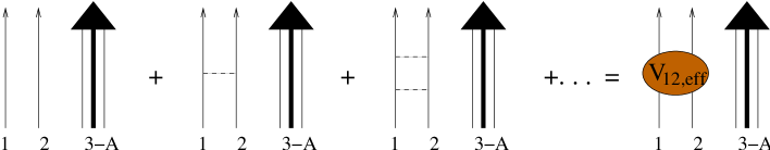
Figure 1: (Color online) Diagrammatic terms kept in ladder approximation of Eq. 6. Nucleons 1 and 2 are interacting via a ladder sum in the presence of spectator nucleons 3-A. Dashed lines represent interactions with $V_{12}$.

We retain from this expansion only the terms that contribute to a ladder summation, as shown diagrammatically in Fig. 1. Here only particles 1 and 2 are interacting via repeated insertions of the potential $V_{12}$, while particles 3 through A are spectator nucleons. This infinite ladder sum is collectively grouped into the expression $V_{12,eff}$. Hence $V_{eff}$ is approximated as

$$V_{eff} \sim \sum_{i<j}^{A}V_{ij,eff}$$ (7)

$$= \frac{A(A-1)}{2}V_{12,eff},$$ (8)

where the $A(A-1)/2$ factor comes from using anti-symmetrised states. Obviously the choice of $ij=12$ in Eq. 8 is arbitrary.

There are three distinct ways in which to do the ladder summation. The first method assumes that the spectator particles are completely irrelevant. They do not contribute in any way to the ladder interactions between particles 1 and 2. Such an approximation is akin to the G-matrix interaction of traditional shell-model calculations. The resulting interaction is completely two-body in nature which, from a computational standpoint, greatly simplifies the problem. Furthermore, the effective interaction is much softer than the original bare $NN$ interaction, thereby reducing the coupling of the high momentum matrix elements to the included space. This softening of the core is a generic property of the ladder sum. Indeed, it can be shown that in the limit of an infinite hard core, matrix elements of this ladder summation are still finiteFetter and Walecka (2003). With these approximations, Eq. 6 becomes

$$V_{12,eff}=\frac{1}{E-Q_{12}T_{12}}Q_{12}+\frac{1}{E-Q_{12}T_{12}}Q_{12}V_{12}\frac{1}{E-Q_{12}T_{12}}Q_{12}+\\ \frac{1}{E-Q_{12}T_{12}}Q_{12}V_{12}\frac{1}{E-Q_{12}T_{12}}Q_{12}V_{12}\frac{1}{E-Q_{12}T_{12}}Q_{12}+\ldots$$ (9)

Note the replacement of $Q$ with $Q_{12}$ in the previous equation. Since the presence of spectator nucleons is completely ignored, the many-body projection operator $Q$ acts only within the two-body sector. This condition is valid only in the $\Lambda=0$ excitation spacesZheng et al. (1995). We label this operator as $Q_{12}$. Since this interaction is only two-body, it is a poor approximation to the original $H_{eff}$, since the latter is an A-body interaction. Furthermore, since $T$ is replaced by $T_{12}$, the energy E can no longer be associated with the energy of the A-body system. Historically, the missing many-body correlations have been ‘mocked’ up by introducing fictitious parameters, such as starting energies $\omega$. These further approximations eliminate any self-consistency, as well as manifest A-body anti-symmetry. Attempts at improving the effective interaction via perturbation have had mixed success as well. Barrett and KirsonBarrett and Kirson (1970) have shown that matrix elements of third order (in G) diagrams can be as large as second order diagrams. These inconsistencies have led shell model practitioners on a more phenomenological track, using effective two-body matrix elements derived by fitting to nuclear spectra. Clearly any underlying connection to the original bare $NN$ interaction has been lost at this point.

Since the included space is defined in terms of many-body states (and not just two-body states) with total HO quanta below $\Lambda$, the actual HO configuration of the spectator nucleons restricts the possible configuration in which the two-nucleon cluster may interact. This is especially true for multi-valued excitation spaces (i.e. $\Lambda>0$). For example, within a $\Lambda\hbar\omega=4\hbar\omega$ included space, a $2\hbar\omega$ spectator state restricts the possible two-body interacting cluster to either $0\hbar\omega$ or $2\hbar\omega$, since the sum of the HO quanta of the spectator and interacting clusters must add to a value $\leq\Lambda=4$. The multiplicity of the two-nucleon state implies that the G-matrix is multivalued. This implicit spectator dependence can be included within the ladder sum by replacing $Q_{12}$ by the full many-body $Q$ within Eq. 9,

$$V_{12,eff}=\frac{1}{E-QT_{12}}Q+\frac{1}{E-QT_{12}}QV_{12}\frac{1}{E-QT_{12}}Q+\\ \frac{1}{E-QT_{12}}QV_{12}\frac{1}{E-QT_{12}}QV_{12}\frac{1}{E-QT_{12}}Q+\ldots$$ (10)

Equation 10 represents the second method for performing the ladder summation. Zheng et al.Zheng et al. (1995) have shown that there are significant improvements to using the multi-valued G-matrix over its single-valued cousin. In particular, the calculated low energy excitation spectrum of certain few-body systems were lowered relative to the ground state when using the multi-valued G, bringing energies into better agreement with experiment. Despite its spectator dependence, however, Eq. 10 still represents a two-body operator since it is diagonal in all spectator quantum numbers. Hence induced multi-particle correlations are still missing.

In the center of mass frame, the relative kinetic energies of the interacting two-nucleon cluster and spectator cluster are correlated. This is especially true for light systems. This cluster recoil can be incorporated into the ladder sum by using the full kinetic energy operator $T$ in Eq. 10,

$$V_{12,eff}=\frac{1}{E-QT}Q+\frac{1}{E-QT}QV_{12}\frac{1}{E-QT}Q+\\ \frac{1}{E-QT}QV_{12}\frac{1}{E-QT}QV_{12}\frac{1}{E-QT}Q+\ldots$$ (11)

Note that since the full $Q$ and $T$ are present, Eq. 11 represents a multi-valued, A-body operator. The A-body nature of this operator implies that some induced multi-particle correlations are being incorporated at this level of approximation. However, these correlations do not come from potential interactions; rather, they stem solely from the fact that the kinetic energies of the clusters are correlated. This is the third and final approximation to $V_{eff}$ (Eq. 5) which can be obtained from a ladder summation. It is also the approximation of $V_{eff}$ that we investigate in this paper.

IV Calculating A-body matrix elements of $V_{12,eff}$

The infinite ladder sum in Eq. 11 can be expressed in closed formLuu et al. (2004),

$$V_{12,eff}=t_{12}-t_{12}G_{0}P\frac{1}{\Gamma_{0}+\Gamma_{\infty}}PG_{0}t_{12},$$ (12)

where

$$G_{0} = \frac{1}{E-T},$$ (13)

$$\Gamma_{0} = PG_{0}P,$$ (14)

$$t_{12} = V_{12}+V_{12}G_{0}t_{12},$$ (15)

$$\Gamma_{\infty} = PG_{0}t_{12}G_{0}P.$$ (16)

This is precisely the leading-order BH term of Ref.Luu et al. (2004). Here $G_{0}$ represents the free many-body propagator, while $\Gamma_{0}$ consists of included-space overlaps of $G_{0}$. The t-matrix for free particles satisfies the Lippman-Schwinger equation that depends on $V_{12}$ and the many-body propagator $G_{0}$, and $\Gamma_{\infty}$ represents included-space overlaps of $t_{12}$ weighted by two insertions of $G_{0}$.

The many-body nature of the operator $V_{12,eff}$ comes directly from the included-space overlaps of $G_{0}t_{12}G_{0}$. In momentum space $t_{12}$ is not only a function of the interacting two-nucleon cluster’s initial and final momenta, $p$ and $p^{\prime}$ respectively, but also of the individual spectator Jacobi momenta $q_{i}$,

$$t_{12}(p^{\prime},p;E-\sum_{i=1}^{A-2}q_{i}^{2}/2M_{n}).$$ (17)

Here $M_{n}$ is the nucleon mass. This dependence on spectator momenta implies that overlaps of this operator are not diagonal in all the spectator’s quantum numbers, and in particular, their principle quantum numbers can change by arbitrary amounts. In principle, calculating included-space many-body matrix elements of this operator would require numerically evaluating A-dimensional nested integrals in momentum space (the same is true in coordinate space). Such integrals can be done via Monte Carlo methods, though these methods would be very computationally taxing and probably inaccurate due to the oscillatory nature of the HO wavefunctions. In Appendix B we show an alternative method in which the multi-dimensional integrals over the spectator nucleons can be reduced to a sum over one-dimensional integrals. The result is valid regardless of the number of spectator nucleons, and is given by

$$\int dq_{1}\cdots dq_{A-2}\ q_{1}^{2}\cdots q_{A-2}^{2}\ R_{n_{1}^{\prime}l_{1}}(q_{1})R_{n_{1}l_{1}}(q_{1})\cdots R_{n_{A-2}^{\prime}l_{A-2}}(q_{A-2})R_{n_{A-2}l_{A-2}}(q_{A-2})\\ \times t_{12}(p^{\prime},p;E-\sum_{i=1}^{A-2}\frac{q_{i}^{2}}{2\mu})=\\ \sum_{m_{1},m^{\prime}_{1},\cdots,m_{A-2},m^{\prime}_{A-2}=0}^{n_{1},n^{\prime}_{1},\cdots,n_{A-2},n^{\prime}_{A-2}}C(m_{1},m^{\prime}_{1},\cdots,m_{A-2},m^{\prime}_{A-2})\\ \times\left[\int_{0}^{\infty}d\rho\ \rho^{A-3+2\Sigma_{i}^{A-2}(l_{i}+m_{i}+m_{i}^{\prime}+1)}e^{-\rho^{2}}t_{12}(p^{\prime},p;E-\frac{\rho^{2}}{2M_{n}b^{2}})\right],$$ (18)

where $b$ is the oscillator parameter and

$$C(m_{1},m^{\prime}_{1},\cdots,m_{A-2},m^{\prime}_{A-2})=\\ (-1)^{\Sigma_{i}(n_{i}+m_{i})}\left[\prod_{i=1}^{A-2}\ \frac{\sqrt{2\Gamma(n_{i}+1)\Gamma(n_{i}+l_{i}+3/2))}}{\Gamma(n_{i}-m_{i}+1)\Gamma(l_{i}+m_{i}+3/2)\Gamma(m_{i}+1)}\right]\\ \times(-1)^{\Sigma_{i}(n^{\prime}_{i}+m^{\prime}_{i})}\left[\prod_{i=1}^{A-2}\ \frac{\sqrt{2\Gamma(n^{\prime}_{i}+1)\Gamma(n^{\prime}_{i}+l_{i}+3/2))}}{\Gamma(n^{\prime}_{i}-m^{\prime}_{i}+1)\Gamma(l_{i}+m^{\prime}_{i}+3/2)\Gamma(m^{\prime}_{i}+1)}\right]\\ \times\left[\prod_{i=2}^{A-2}\frac{\Gamma(l_{i}+m_{i}+m_{i}^{\prime}+3/2)\Gamma(\sum_{j=1}^{i-1}(l_{j}+m_{j}+m_{j}^{\prime}+1)+\frac{i-1}{2})}{2\Gamma(l_{i}+m_{i}+m_{i}^{\prime}+\sum_{j=1}^{i-1}(l_{j}+m_{j}+m_{j}^{\prime}+1)+\frac{i+2}{2})}\right].$$ (19)

In Eq. 19 the first two products run over all spectator nucleons (i.e. $i$=1 to $A$-2). Equation 18 utilized the fact that matrix elements of $t_{12}$ are diagonal in the spectator’s orbital quantum numbers $l_{i}$ (see Appendix B), but not their principle quantum numbers. The right hand side (RHS) of Eq. 18 represents a significant simplification to the original multi-dimensional integrals, since the one-dimensional integrals of the RHS can be done quickly and accurately. The coefficients $C(m_{1},m^{\prime}_{1},\cdots,m_{A-2},m^{\prime}_{A-2})$ are known analytically and can be pre-computed and stored.

IV.1 Dependence of $t_{12}$ on spectator nucleons

Equation 18 is only a function of the initial and final momenta of the interacting two-nucleon cluster (i.e. nucleons one and two). However, its functional form depends implicitly on the number of spectator nucleons and their initial HO momentum distribution. In some sense, $\overline{t_{12}}$ represents the average interaction of particles one and two under the influence of the spectator’s momentum distributions. It is not a mean-field interaction, since $\overline{t_{12}}$ is not derived from any interactions with the spectator nucleons. We will discuss this point in more detail later.

Figure 2 shows this spectator dependence of the operator $b\hbar\omega p^{\prime 2}\overline{G_{0}(p^{\prime};E)t_{12}(p^{\prime},p;E)G_{0}(p;E)}p^{2}$, which is dimensionless. Note that $\omega$ is the HO frequency, defined by $\hbar\omega=\hbar^{2}/M_{N}b^{2}$, where $M_{N}$ is the nucleon mass. We plot this quantity rather than $\overline{t_{12}(p^{\prime},p;E)}$ since it is more relevant for our calculations and more visually instructive. All plots within Fig. 2 are for the case when $t_{12}$ is in the ${}^{1}S_{0}$ channel, plotted against initial and final dimensionless momenta $bp$ and $bp^{\prime}$, respectively. Furthermore, all plots were calculated with E=-20 MeV and $b$=1.2 fm. Plot (a) shows this operator when there are no spectator nucleons present. In this case $t_{12}$ is the standard two-body t-matrix. Plot (b) shows how this operator is modified after integrating out the presence of two spectator nucleon in the lowest allowed relative Jacobi configuration, the $0s$ state. Plot (c) shows the effect of integrating out three spectator nucleons, two of which are in $0s$ states and one in a $0p$ state. Finally, plot (d) shows how the interaction is altered with the presence if four spectator nucleons are integrated out. In this case, two of the nucleons are in relative $0s$ states, and two are in the relative $0p$ states.

The physical interpretations of the troughs and peaks seen in Fig. 2 are difficult to explain due to the complicated structure of the operator $\overline{G_{0}(p^{\prime};E)t_{12}(p^{\prime},p;E)G_{0}(p;E)}$. What is clear is that the inclusion of additional spectator nucleons softens this operator. This is consistent with the fact that the possible configurations of the interacting two-nucleon cluster are reduced with increasing numbers of spectator nucleons.

V Results

In all our calculations we use the Argonne $v_{18}$ and $v^{\prime}_{8}$ potentialsWiringa et al. (1995) (Av18 and Av8’) for our $NN$ interactions. Furthermore, we ignore isospin symmetry breaking effects included in the Av18 potential since this is a small effect. Table 1 shows the dimensions of the $\Lambda=0,2$ included-spaces for the ground state quantum numbers of different few-body systems considered in this paper. Since the dimensions are very small, our calculations do not demand extravagant computing resources and can be done very quickly. To construct our included-space anti-symmetrised HO Jacobi wavefunctions, we use a modified version of the routine manyeff outlined in Ref.Navratil et al. (2000). We make our comparisons with GFMC and NCSM calculations, and show experimental results solely as reference points.

V.1 S-shell nuclei

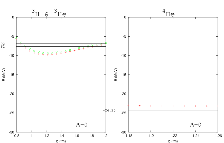
Figure 3: (Color online) S-shell results for $\Lambda=0$ included spaces. Points correspond to our calculations, whereas solid lines correspond to the ‘exact’ results taken from Ref.Nogga et al. (2002). In the three-body system, the upper and lower set of points refer to ³He and ³H, respectively. We do not show results for ²H, since all calculated points lie on the exact theoretical result, regardless of $b$. Calculations were done with the Av18 potential.

Figure 3 shows our results of using $V_{12,eff}$ on s-shell nuclei. All calculations were done in $\Lambda=0$ included spaces and with the Av18 potential. Our results are displayed by points, while the ‘exact’ theoretical results are taken from Ref.Nogga et al. (2002) and displayed as solid lines. For the three-body system, the upper and lower set of points refer to ³He and ³H, respectively. Note that for ⁴He, the plotted range of $b$ values is much smaller.

The ²H system is special since in this two-body system there are no spectator nucleons. The ladder sum of Fig. 1 is exact in this case, meaning that $V_{12,eff}$ is not an approximation but corresponds to the exact effective interaction. Thus any calculations of the two-body system cannot depend on $b$, as this is an intrinsic parameter of the HO basis and has nothing to do with the $NN$ interaction. Indeed, all our ²H calculations lie on the exact theoretical binding energy, regardless of the oscillator parameter $b$ (as well as size $\Lambda$). Hence, we do not show this case in Fig. 3.

The variation of the binding energy with $b$ in the three-body system and higher is a key indicator that $V_{12,eff}$ is only approximative for these systems. Furthermore, the fact that the calculated binding energies can overbind for certain values of $b$, as shown in the three-body system, shows that this approximation is not variational. For the alpha particle, our results underbind by $\sim 1$ MeV.

V.2 P-shell nuclei

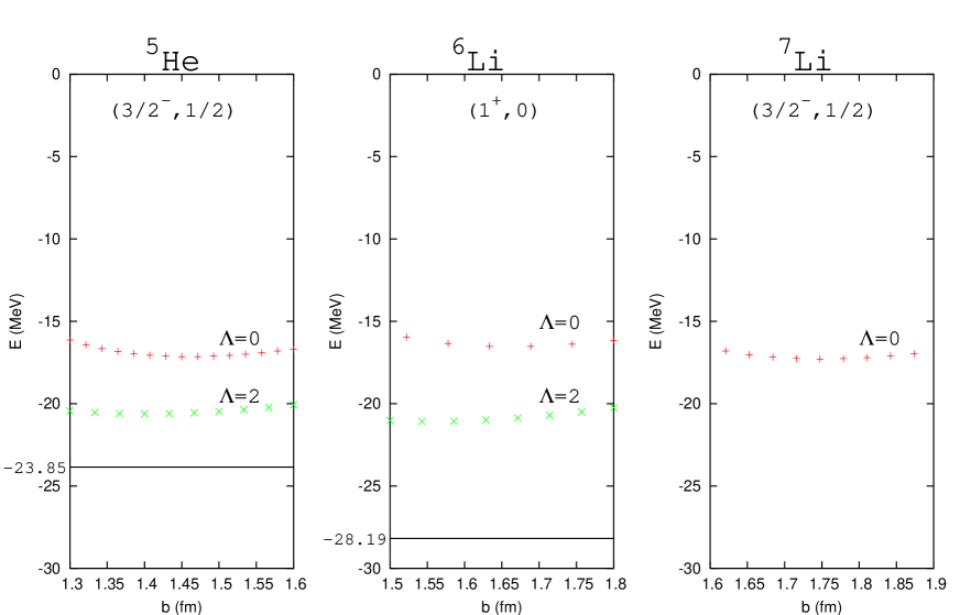
Figure 4: (Color online) Same as in Fig. 3, but for p-shell ground states using Av8’. Solid lines correspond to results taken from Ref.Pieper et al. (2004).

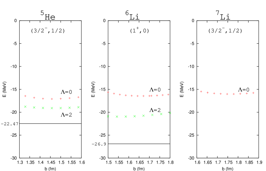
Figure 5: (Color online) Same as in Fig. 4, but using Av18.

Figure 4 shows our results for the ground state binding energies for ⁵He, ⁶Li, and ⁷Li using the Av8’ potential. Again, our results are displayed with points, while the ‘exact’ theoretical binding energies are taken from Refs.Pieper et al. (2004) and displayed by solid lines. For the seven-body system, the calculated GFMC binding energy is -33.56 MeV, which is below the plotted range in Fig. 4. Numbers in parenthesis refer to the quantum numbers (J^π,T). For the five- and six-body systems, we show calculations for both $\Lambda=0$ and $\Lambda=2$ included spaces. For the p-shell nuclei presented here our results underbind for all values of $b$. We plot our results where our calculated binding energies approach closest to the exact theoretical results. The selected ranges of $b$ in Fig. 4 reflect this fact. Figure 5 shows the same results using the Av18 potential.

Since the $\Lambda=0$ calculations of these p-shell nuclei all underbind, they are susceptible to cluster breakup. Furthermore, their calculated binding energies are nearly degenerate. We do not have a satisfactory explanation for this behavior. This apparent degeneracy is broken in the $\Lambda=2$ calculations of the five- and six-body systems. We have not performed any $\Lambda=2$ calculations for the seven-body system due to time and computer limitations.

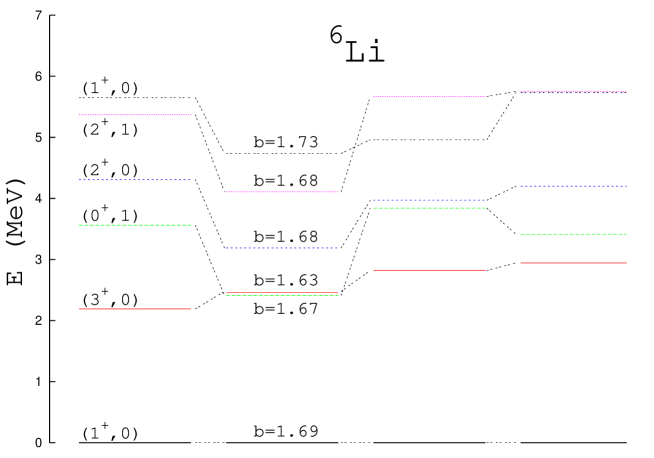
Figure 6: (Color online) Excited spectrum of ⁶Li using Av8’.

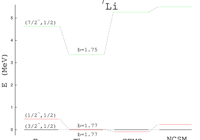
Figure 7: (Color online) Excited spectrum of ⁷Li using Av8’.

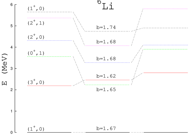
Figure 8: (Color online) Excited spectrum of ⁶Li using Av18.

P-shell nuclei have richer structure than their s-shell counterparts due to the existence of excited states. In Figs. 6-7 we show the excited spectrum of ⁶Li and ⁷Li using the Av8’ potential. We also show the experimental spectrum to provide reference points, but stress that our results should only be compared to GFMC/NCSM results only. All BH calculations were done in $\Lambda=0$ included spaces. The quoted $b$ values are taken at the minimum binding energy for each level. The Av18 results are shown in Figs. 8-9.

Our $\Lambda=0$ calculations of excited spectra fall within the range of GFMC and NCSM results. We note that the NCSM ⁶Li calculations were performed in a $\Lambda$=14 included space using $\hbar\Omega=11$ MeV ($b$=1.94 fm) and gave 28.08 MeV binding for the ground state of ⁶Li using Av8’. The excitation energies of the $(2^{+},0)$ and, in particular, of the $(1^{+}_{2},0)$ states were not converged yet and are still decreasing with increasing $\Lambda$. The NCSM ⁷Li results are taken from Ref. Navratil and Ormand (2003). In general our level orderings correlate with those of GFMC and NCSM calculations as well. However, certain levels are inverted, such as the (3⁺,0)-(0⁺,1) states of ⁶Li and the (3/2^-,1/2)-(1/2^-,1/2) states of ⁷Li. These particular levels are sensitive to the strength of the spin-orbit interaction in the $NN$ interaction, which to date, is poorly represented in all potential models. Clearly our approximation of $V_{eff}$ in these limiting included spaces exacerbates this issue. The energy differences between using Av18 and Av8’ are typically less than $\sim 200$ KeV.

VI Convergence Issues

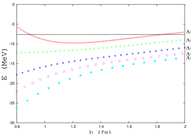
Figure 10: (Color online) Dependence of ³H on models space size $\Lambda$ and oscillator parameter $b$ using Av18. The solid line is the exact ³H binding energy with the Av18 potential.

The $\Lambda=2$ calculated binding energies for the five- and six-body systems of Figs. 4-5 are closer to the exact answers compared to the $\Lambda=0$ results, and the dependence on $b$ is somewhat flatter. This suggests some sort of convergence with increasing $\Lambda$. Indeed, as $\Lambda\rightarrow\infty$, one has that $P\rightarrow 1$, giving $V_{12,eff}\rightarrow V_{12}$. Hence in this limit the calculated binding energies are guaranteed to converge to the exact answers. However, we caution that since we are working in such small included spaces, such limiting behavior might not be seen until $\Lambda$ becomes much larger. Furthermore, the argument above does not give any information on how quickly the binding energies converge to the exact answer. For example, larger model space calculations of the ³H (Fig. 10) do not show a systematic convergence. This is in direct contrast to NCSM calculations, where there is definite convergence as the included space is increasedNavratil et al. (2000). A possible explanation for this difference is in the incorporation of a confining HO mean-field potential in NCSM calculations. The starting bare Hamiltonian for NCSM calculations is

$$H^{\rm NCSM}=H+T_{c.m.}+U^{\rm HO}_{c.m.},$$

where $H$ is given by Eq. (2) and $T_{c.m.}+U^{\rm HO}_{c.m.}$ is the c.m. harmonic oscillator Hamiltonian. In principle, the addition of a confining HO Hamiltonian (which is in the end subtracted from the effective Hamiltonian in any case) does not alter the final answer of the many-body problem, as long as the effective interaction is solved to a high level of accuracy. Indeed, we argue that the inclusion of a confining mean-field increases the rate of convergence as the size of the included-space is increased. Since our BH calculations lack any confining mean-field (e.g. $U^{\rm HO}_{c.m.}$), our convergence with increasing $\Lambda$ is hindered.

VII Conclusion

The exponentially increasing complexity of the many-body Hilbert space motivates the use of effective interactions in truncated included spaces. Unfortunately, the exact effective interaction $H_{eff}$ is as difficult to deal with as the original infinite-Hilbert space problem. Hence some form of approximation must be made to $H_{eff}$, or more specifically, to $V_{eff}$. In Sect. III we showed a particular approximation of $V_{eff}$ that was obtained by summing ladder diagrams to all orders, giving $V_{12,eff}$. We argued that our approximation of $V_{eff}$, one in which spectator dependence and cluster recoil are manifestly included, was a natural extension of the single-valued G-matrix of traditional shell model calculations and the multi-valued G-matrix of Ref.Zheng et al. (1995). Our approximation of $V_{eff}$ is equivalent to the leading order term of the BH expansion of Ref.Luu et al. (2004).

Because we include the effects of cluster recoil, our approximation of $V_{eff}$ is an A-body operator, as opposed to the two-body nature of the G-matrix interactions mentioned above. In Sect. IV and Appendix B we showed how A-body matrix elements of $V_{12,eff}$ can be easily calculated by transforming the A-dimensional nested integrals into a sum over one-dimensional integrals. The result is valid for any A-body system and can be computed quickly and accurately. We showed that by integrating over the spectator degrees of freedom, we could define an average residual interaction for the interacting two-nucleon cluster that depended on the initial HO momentum configurations of the spectator nucleons. Figure 2 shows how this average interaction in the ¹S₀ channel changes as the number of spectator nucleons is increased.

Finally, in Sect. V we showed our results of using $V_{12,eff}$ in s- and some p-shell nuclei for the smallest allowed included spaces. All our calculations produced stationary solutions (i.e. negative binding energies). Our s-shell results show good agreement with exact theoretical answers. In particular, the alpha particle is underbound by only $\sim 1$ MeV. On the other hand, our p-shell results all severely underbind in $\Lambda=0$ included spaces, and are therefore susceptible to cluster breakup. The excitation spectra of ⁶Li and ⁷Li fell within the ranges calculated by GFMC and NCSM methods. The level orderings correlated to some extent with these methods as well, though level inversions do exist. We argued that these level inversions were closely related to the weak spin-orbit interactions of the potential models used in our calculations, which were further exacerbated by our approximation of $V_{eff}$ in such small included spaces.

For both ⁵He and ⁶Li, we extended our calculations to $\Lambda=2$ included spaces (see Figs. 3-4), and some semblance of convergence was observed. We caution, however, that any apparent convergence in such small spaces is not definitive. Indeed, for the case of ³H, convergence was not seen as the size of the included-space increased, as shown in Fig. 6. This is in direct contrast to NCSM calculations. Though our calculations are, in a sense, more sophisticated than NCSM calculations, our results are no better for $\Lambda\geq 2$. We argued in Sec. VI that the lack of a confining ‘mean-field’ potential was the most likely reason for our poor convergence.

As mentioned in the previous section, our calculations were not too computationally demanding since we worked within the smallest allowed included spaces. Indeed, we were able to perform all our calculations on a single Unix box. Calculations on higher A-body systems, or on much larger included spaces, will require that our calculations become parallelized, which we hope to do in the near future. It would be interesting to see if the $\Lambda=0$ ‘degeneracy’ persists for larger p-shell nuclei. To tackle our convergence issues, we intend to incorporate a ‘mean-field’ potential into our future calculations.

Appendix A A-body matrix elements of $T_{eff}$

The relevant expression in Jacobi coordinates is

$$<n^{\prime}_{1}l^{\prime}_{1}\cdots n^{\prime}_{A-1}l^{\prime}_{A-1}|\frac{1}{E-T}|n_{1}l_{1}\cdots n_{A-1}l_{A-1}>=\delta_{l^{\prime}_{1},l_{1}}\cdots\delta_{l^{\prime}_{A-1},l_{A-1}}\\ \times\int dp_{1}\cdots dp_{A-1}R^{*}_{n^{\prime}_{1}l_{1}}(p_{1})\cdots R^{*}_{n^{\prime}_{A-1}l_{A-1}}(p_{A-1})\frac{p_{i}^{2}\cdots p_{A-1}^{2}}{E-\sum_{i=1}^{A-1}\frac{p_{i}^{2}}{2M_{n}}}R_{n_{1}l_{1}}(p_{1})\cdots R_{n_{A-1}l_{A-1}}(p_{A-1}),$$ (20)

where $R_{nl}(p)$ is the HO radial wavefunction in momentum space. Replacing the radial integrals by their series expansion and changing to dimensionless variables $x_{1},\ldots,x_{A-1}$, Eq. 20 becomes

$$\delta_{l^{\prime}_{1},l_{1}}\cdots\delta_{l^{\prime}_{A-1},l_{A-1}}\sum_{m_{1},m^{\prime}_{1},\cdots,m_{A-1},m^{\prime}_{A-1}=0}^{n_{1},n^{\prime}_{1},\cdots,n_{A-1},n^{\prime}_{A-1}}A(m_{1},m^{\prime}_{1},\cdots,m_{A-1},m^{\prime}_{A-1})\\ \times\left[\int dx_{1}\cdots dx_{A-1}e^{-(x_{1}^{2}+\cdots+x_{A-1}^{2})}\frac{x_{1}^{2(l_{1}+m_{1}+m_{1}^{\prime}+1)}\cdots x_{A-1}^{2(l_{A-1}+m_{A-1}+m_{A-1}^{\prime}+1)}}{E-\frac{1}{2M_{n}b^{2}}\sum x_{i}^{2}}\right],$$ (21)

where

$$A(m_{1},m^{\prime}_{1},\cdots,m_{A-1},m^{\prime}_{A-1})=\\ (-1)^{\Sigma_{i}(n_{i}+m_{i})}\left[\prod_{i=1}^{A-1}\ \frac{\sqrt{2\Gamma(n_{i}+1)\Gamma(n_{i}+l_{i}+3/2))}}{\Gamma(n_{i}-m_{i}+1)\Gamma(l_{i}+m_{i}+3/2)\Gamma(m_{i}+1)}\right]\\ \times(-1)^{\Sigma_{i}(n^{\prime}_{i}+m^{\prime}_{i})}\left[\prod_{i=1}^{A-1}\ \frac{\sqrt{2\Gamma(n^{\prime}_{i}+1)\Gamma(n^{\prime}_{i}+l_{i}+3/2))}}{\Gamma(n^{\prime}_{i}-m^{\prime}_{i}+1)\Gamma(l_{i}+m^{\prime}_{i}+3/2)\Gamma(m^{\prime}_{i}+1)}\right].$$ (22)

The integral in Eq. 20 can be evaluated by first changing variables to (A-1)-dimensional polar coordinates, $\rho,\theta_{A-5},\ldots,\theta_{1},\phi$, where $0\leq\phi\leq 2\pi$, and $0\leq\theta_{i}\leq\pi$:

$$x_{1}= \ \rho\ cos\phi\ sin\theta_{1}\ sin\theta_{2}\cdots sin\theta_{A-5}$$ (23)

$$x_{2}= \ \rho\ sin\phi\ sin\theta_{1}\ sin\theta_{2}\cdots sin\theta_{A-5}$$

$$x_{3}= \ \rho\cos\theta_{1}\ sin\theta_{2}\cdots sin\theta_{A-5}$$

$$\vdots= \ \vdots$$

$$x_{i}= \ \rho\ cos\theta_{i-2}\ sin\theta_{i-1}\cdots sin\theta_{A-5}$$

$$\vdots= \ \vdots$$

$$x_{A-1}= \ \rho\ cos\theta_{A-5}$$

$$\rho^{2}= \ \sum x_{i}^{2}.$$

The infinitesimal volume element is

$$dx_{1}\cdots dx_{A-1}=\ \rho^{A-4}\ sin^{A-5}\theta_{A-5}\cdots sin\theta_{1}\ d\rho\ d\theta_{A-5}\cdots d\theta_{1}\ d\phi.$$

With these change of variables, the integral in Eq. 20 becomes

$$\left[\int_{0}^{\pi/2}(cos\phi)^{2(l_{1}+m_{1}+m_{1}^{\prime}+1)}(sin\phi)^{2(l_{2}+m_{2}+m_{2}^{\prime}+1)}d\phi\right]\\ \times\left[\int_{0}^{\pi/2}(cos\theta_{1})^{2(l_{3}+m_{3}+m_{3}^{\prime}+1)}(sin\theta_{1})^{2\sum_{i=1}^{2}(l_{i}+m_{i}+m_{i}^{\prime}+1)+1}d\theta_{1}\right]\\ \cdots\times\left[\int_{0}^{\pi/2}(cos\theta_{A-5})^{2(l_{A-1}+m_{A-1}+m_{A-1}^{\prime}+1)}(sin\theta_{A-5})^{2\sum_{i=1}^{A-2}(l_{i}+m_{i}+m_{i}^{\prime}+1)+A-5}d\theta_{A-5}\right]\\ \times\left[\int_{0}^{\infty}d\rho\ e^{-\rho^{2}}\frac{\rho^{A-2+2\sum_{i=1}^{A-1}(l_{i}+m_{i}+m_{i}^{\prime}+1)}}{E-\frac{\rho^{2}}{2M_{n}b^{2}}}\right].$$ (24)

Note the limits of integration. All the angular integrals and the integral over $\rho$ can be expressed analytically,

$$\int_{o}^{\pi/2}d\theta\ cos^{\alpha}\theta\ sin^{\beta}\theta = \frac{\Gamma(\frac{\alpha+1}{2})\Gamma(\frac{\beta+1}{2})}{2\Gamma(\frac{\alpha+\beta}{2}+1)},$$ (25)

$$\int_{0}^{\infty}d\rho\ e^{-\rho^{2}}\frac{\rho^{2\alpha+1}}{\epsilon-\rho^{2}} = \frac{(-1)^{\alpha+1}}{2}\epsilon^{\alpha}e^{-\epsilon}\ \Gamma(-\alpha,-\epsilon)\Gamma(\alpha+1).$$ (26)

Plugging Eqs. 24- 26 into Eq. 21 gives the final result,

$$<n^{\prime}_{1}l^{\prime}_{1}\cdots n^{\prime}_{A-1}l^{\prime}_{A-1}|\frac{1}{E-T}|n_{1}l_{1}\cdots n_{A-1}l_{A-1}>=\\ \delta_{l^{\prime}_{1},l_{1}}\cdots\delta_{l^{\prime}_{A-1},l_{A-1}}\frac{2}{\hbar\omega}\sum_{m_{1},m^{\prime}_{1},\cdots,m_{A-1},m^{\prime}_{A-1}=0}^{n_{1},n^{\prime}_{1},\cdots,n_{A-1},n^{\prime}_{A-1}}B(m_{1},m^{\prime}_{1},\cdots,m_{A-1},m^{\prime}_{A-1})\\ \times\left[\frac{(-1)^{\alpha+1}}{2}\left(\frac{2E}{\hbar\omega}\right)^{\alpha}e^{-\frac{2E}{\hbar\omega}}\ \Gamma(-\alpha,-\frac{2E}{\hbar\omega})\Gamma(\alpha+1)\right],$$ (27)

where $\alpha=(A-3)/2+\sum_{i}(l_{i}+m_{i}+m^{\prime}_{i}+1)$ and

$$B(m_{1},m^{\prime}_{1},\cdots,m_{A-1},m^{\prime}_{A-1})=\\ (-1)^{\Sigma_{i}(n_{i}+m_{i})}\left[\prod_{i=1}^{A-1}\ \frac{\sqrt{2\Gamma(n_{i}+1)\Gamma(n_{i}+l_{i}+3/2))}}{\Gamma(n_{i}-m_{i}+1)\Gamma(l_{i}+m_{i}+3/2)\Gamma(m_{i}+1)}\right]\\ \times(-1)^{\Sigma_{i}(n^{\prime}_{i}+m^{\prime}_{i})}\left[\prod_{i=1}^{A-1}\ \frac{\sqrt{2\Gamma(n^{\prime}_{i}+1)\Gamma(n^{\prime}_{i}+l_{i}+3/2))}}{\Gamma(n^{\prime}_{i}-m^{\prime}_{i}+1)\Gamma(l_{i}+m^{\prime}_{i}+3/2)\Gamma(m^{\prime}_{i}+1)}\right]\\ \times\left[\prod_{i=2}^{A-1}\frac{\Gamma(l_{i}+m_{i}+m_{i}^{\prime}+3/2)\Gamma(\sum_{j=1}^{i-1}(l_{j}+m_{j}+m_{j}^{\prime}+1)+\frac{i-1}{2})}{2\Gamma(l_{i}+m_{i}+m_{i}^{\prime}+\sum_{j=1}^{i-1}(l_{j}+m_{j}+m_{j}^{\prime}+1)+\frac{i+2}{2})}\right].$$ (28)

Appendix B Integrating out spectator degrees of freedom

The relevant expression here is

$$<p^{\prime};n_{1}^{\prime}l_{1}^{\prime},\cdots,n_{A-2}^{\prime}l_{A-2}^{\prime}|\hat{F}|p;n_{1}l_{1},\cdots,n_{A-2}l_{A-2}>,$$ (29)

where the interacting two-nucleon initial and final momenta are $p$ and $p^{\prime}$, respectively, and the spectator quantum numbers are denoted with subscripts that run from $1$ through $A-2$.. $\hat{F}$ is some operator that depends only on $p$, $p^{\prime}$, and $\sum_{i}q_{i}^{2}$, where $q_{i}$ are the spectator momenta. $G_{0}$, $t_{12}$, and $G_{0}t_{12}G_{0}$ are three examples of such an operator. Since $F$ only depends on $q_{i}^{2}$, which is a scalar, it cannot change the orbital quantum numbers of the spectator nucleons. Hence Eq. 29 becomes

$$\delta_{l_{1}^{\prime},l_{1}}\cdots\delta_{l_{A-2}^{\prime},l_{A-2}}\\ \times\int dq_{1}\cdots dq_{A-2}q_{1}^{2}\cdots q_{A-2}^{2}R^{*}_{n_{1}^{\prime}l_{1}}(q_{1})R_{n_{1}l_{1}}(q_{1})\cdots R^{*}_{n_{A-2}^{\prime}l_{A-2}}(q_{A-2})R_{n_{A-2}l_{A-2}}(q_{A-2})\\ \times F(p,p^{\prime};\sum_{i=1}^{A-2}q_{i}^{2}).$$ (30)

Equation 30 is very similar to Eq. 20. Indeed, we can follow a similar procedure outlined in the previous section to come to our desired result. Repeating the steps from Eq. 21 through Eq. 26, but with a change of variables to (A-2)-dimensional polar coordinates rather than (A-1), gives

$$\delta_{l_{1}^{\prime},l_{1}}\cdots\delta_{l_{A-2}^{\prime},l_{A-2}}\sum_{m_{1},m^{\prime}_{1},\cdots,m_{A-2},m^{\prime}_{A-2}=0}^{n_{1},n^{\prime}_{1},\cdots,n_{A-2},n^{\prime}_{A-2}}C(m_{1},m^{\prime}_{1},\cdots,m_{A-2},m^{\prime}_{A-2})\\ \times\left[\int_{0}^{\infty}d\rho\ \rho^{A-3+2\Sigma_{i}^{A-2}(l_{i}+m_{i}+m_{i}^{\prime}+1)}e^{-\rho^{2}}F(p^{\prime},p;\frac{\rho^{2}}{b^{2}})\right],$$ (31)

where $b$ is the oscillator parameter and

$$C(m_{1},m^{\prime}_{1},\cdots,m_{A-2},m^{\prime}_{A-2})=\\ (-1)^{\Sigma_{i}(n_{i}+m_{i})}\left[\prod_{i=1}^{A-2}\ \frac{\sqrt{2\Gamma(n_{i}+1)\Gamma(n_{i}+l_{i}+3/2))}}{\Gamma(n_{i}-m_{i}+1)\Gamma(l_{i}+m_{i}+3/2)\Gamma(m_{i}+1)}\right]\\ \times(-1)^{\Sigma_{i}(n^{\prime}_{i}+m^{\prime}_{i})}\left[\prod_{i=1}^{A-2}\ \frac{\sqrt{2\Gamma(n^{\prime}_{i}+1)\Gamma(n^{\prime}_{i}+l_{i}+3/2))}}{\Gamma(n^{\prime}_{i}-m^{\prime}_{i}+1)\Gamma(l_{i}+m^{\prime}_{i}+3/2)\Gamma(m^{\prime}_{i}+1)}\right]\\ \times\left[\prod_{i=2}^{A-2}\frac{\Gamma(l_{i}+m_{i}+m_{i}^{\prime}+3/2)\Gamma(\sum_{j=1}^{i-1}(l_{j}+m_{j}+m_{j}^{\prime}+1)+\frac{i-1}{2})}{2\Gamma(l_{i}+m_{i}+m_{i}^{\prime}+\sum_{j=1}^{i-1}(l_{j}+m_{j}+m_{j}^{\prime}+1)+\frac{i+2}{2})}\right].$$ (32)

Note that the integral in Eq. 31 cannot be determined analytically, as in the previous section. However, it can be numerically evaluated quickly and accurately.

Table 1: Dimensions of $\Lambda=0,2$ included spaces for different few-body ground states.

$\Lambda$	2H	3H/3He	4He	5He	6Li	7Li
0	1	1	1	1	3	5
2	3	5	5	26	48	185

Figure 2: (Color online) Spectator dependence of $\overline{G_{0}t_{12}G_{0}}$. All axes are dimensionless. Plot (a) is calculated with no spectator nucleons. Plot (b) includes two extra spectator nucleons on top of the interacting pair. In this case, the Jacobi relative angular momentum for these nucleons are in the $0s$ states. Plot (c) and (d) include a third and fourth nucleon, respectively, in the Jacobi relative $0p$ states.

Figure 9: (Color online) Excited spectrum of ⁷Li using Av18.