HBT Interferometry: Historical Perspective

Abstract

I review the history of HBT interferometry, since its discovery in the mid 50’s, up to the recent developments and results from BNL/RHIC experiments. I focus the discussion on the contributions to the subject given by members of our Brazilian group.

I I. Introduction

I will discuss here the fascinating method invented decades ago, which turned into a very active field of investigation up to the present. This year, we are celebrating the $50^{th}$ anniversary of the first publication of the phenomenon observed through this method. In this section, I will briefly tell the story about the phenomenon in radio-astronomy, the subsequent observation of a similar one outside its original realm, and many a posteriori developments in the field, up to the present.

I.1 I.1  HBT

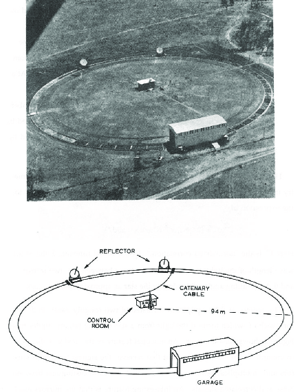
Figure 1: Aerial photo and illustration of the original HBT apparatus. They have been extracted from Ref.gold .

HBT interferometry, also known as two-identical-particle correlation, was idealized in the 1950 s by Robert Hanbury-Brown, as a means to measuring stellar radii through the angle subtended by nearby stars, as seen from the Earth’s surface.

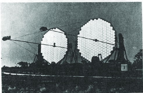
Figure 2: Picture of the two telescopes used in the HBT experiments. The figure was extracted from Ref.gold .

Before actually performing the experiment, Hanbury-Brown invited Richard Q. Twiss to develop the mathematical theory of intensity interference (second-order interference)HBT . A very interesting aspect of this experiment is that it was conceived by both physicists, who also built the apparatus themselves, made the experiment in Narrabri, Australia, and finally, analyzed the data. Nowadays, the experiments doing HBT at the RHIC/BNL accelerator have hundreds of participants. We could briefly summarize the experiment by informing that it consisted of two mirrors, each one focusing the light from a star onto a photo-multiplier tube. An essential ingredient of the device was the correlator, i.e., an electronic circuit that received the signals from both mirrors and multiplied them. As Hanbury-Brown himself described it, they “ … collected light as rain in a bucket … ”, there was no need to form a conventional image: the (paraboloidal) telescopes used for radio-astronomy would be enough, but with light-reflecting surfaces. The necessary precision of the surfaces was governed by maximum permissible field of view. The draw-back they had to face in the first years was the skepticism of the community about the correctness of the results. Some scientists considered that the observation could not be real because it would violate Quantum Mechanics. In reality, in 1956, helped by Purcell purcell , they managed to show that it was the other way round: not only the phenomenon existed, but it also followed from the fact that photons tended to arrive in pairs at the two correlators, as a consequence of Bose-Einstein statistics. A very interesting review about these early years was written by Gerson Goldhabergold , one of the experimentalists responsible for discovering the identical particle correlation in the opposite realm of HBT: the microcosmos of high energy collisions.

I.2 I.2  GGLP

In 1959, Goldhaber, Goldhaber, Lee and Pais performed an experiment at the Bevalac/LBL, in Berkeley, CA, USA, aiming at the discovery of the $\rho^{0}$ resonanceGGLP . In the experiment, they considered $\bar{p}p$ collisions, at 1.05 GeV/c. They were searching for the resonance by means of the decay $\rho^{0}\rightarrow\pi^{+}\pi^{-}$, by measuring the unlike pair, $\pi^{+}\pi^{-}$, mass-distribution and comparing it with the ones for like pairs, $\pi^{\pm}\pi^{\pm}$. Afterwards, they concluded that there was not enough statistics for establishing the existence of $\rho^{0}$. Nevertheless, they observed an unexpected angular correlation among identical pions! Later, in 1960, they successfully reproduced the empirical angular distribution by a detailed multi-$\pi$ phase-space calculation using symmetrized wave functions for LIKE particles. Being so, they concluded the effect was a consequence of the Bose-Einstein nature of $\pi^{+}\pi^{+}$ and $\pi^{-}\pi^{-}$. They were not aware of the experiment Hanbury-Brown and Twiss had performed previously. Thus, they had discovered, by chance, the counterpart of the HBT effect in high energy collisions. They parameterized the observed correlation as:

$$C(Q^{2}) = 1+e^{-Q^{2}r^{2}}=1+e^{(q^{2}_{0}-{\bf q}^{2})r^{2}}$$ (1)

$$Q^{2} = -q^{2}=-(k_{1}-k_{2})^{2}=M^{2}_{12}-(m_{1}+m_{2})^{2}\;.$$

The Gaussian form in the above equation, and several of its variant options, would be widely used in the years to come, mainly by the experimentalists, due to the simplicity of the emission source and analytical results allowed by this profile. We will see which are the parameters and interpretations derived from it in a while.

I.3 I.3  SIMPLE PICTURE

At this point, it is natural to ask the question: How to understand interferometry, or two-particle correlation, in a simple way? First of all, we should anticipate that it follows from considering two essential points: the adequate quantum statistics and chaotically emitting sources, which was already emphasized by Bartknik and Rza̧$\dot{z}$ewskibart . Let me illustrate it by a simple example of only two point sources, as shown in Fig.3:

Figure 3: Simplified picture: two point sources, I and II, emit quanta considered as plane waves, which are observed in detectors A and B, respectively, with momenta $k_{1}^{\mu}$ and $k_{2}^{\mu}$. Since the quanta are indistinguishable, there are two possible combinations for this observation, illustrated by the two continuous and the two dashed lines.

The amplitude for the process can be written as

$$A(k_{1},k_{2}) = \frac{1}{\sqrt{2}}[e^{-ik_{1}.(x_{A}-x_{1})}e^{i{\phi_{1}}}e^{-ik_{2}.(x_{B}-x_{2})}e^{i{\phi_{2}}}$$ (2)

$${\bf\pm}\;e^{-ik_{1}.(x_{A}-x_{2})}e^{i{\phi^{\prime}_{2}}}e^{-ik_{2}.(x_{B}-x_{1})}e^{i{\phi^{\prime}_{1}}}],\;$$

where the ($+$) sign refers to bosons and the ($-$) one, to fermions. In the above equation, $\phi_{i}$ corresponds to an aleatory phase associated to each independent emission (completely chaotic sources), i.e., one phase at random in each emission. These phases are also considered to be independent on the momenta $k$ of the emitted quanta.

The probability for a joint observation of the two quanta with momenta $k_{1}$ and $k_{2}$ is given by

$$P_{2}(k_{1},k_{2})=\langle|A(k_{1},k_{2})|^{2}\rangle=$$ (3)

$$= \frac{1}{2}[2\pm(e^{i(k_{1}-k_{2}).(x_{1}-x_{2})}{\langle}e^{\pm i({\phi_{1}}+{\phi_{2}}-{\phi^{\prime}_{1}}-{\phi^{\prime}_{2}})}{\rangle}+c.c.)]$$

$$= 1\pm\cos[(k_{1}-k_{2}).(x_{1}-x_{2})].$$

The emission being chaotic, we have to consider an average over random phases, i.e.,

$${\langle}e^{\pm i({\phi_{1}}+{\phi_{2}}-{\phi^{\prime}_{1}}-{\phi^{\prime}_{2})}}{\rangle}=\delta_{{\phi_{1}\phi^{\prime}_{1}}}\delta_{{\phi_{2}\phi^{\prime}_{2}}}+\delta_{{\phi_{1}\phi^{\prime}_{2}}}\delta_{{\phi_{2}\phi^{\prime}_{1}}}\;.$$ (4)

The two-particle correlation function can be written as

$$C(k_{1},k_{2})={{P_{2}(k_{1},k_{2})}\over{P_{1}(k_{1})P_{1}(k_{2})}}=1\pm\cos[(k_{1}-k_{2}).(x_{1}-x_{2})]\;,$$ (5)

where $P_{i}(k_{i})$ is the single-inclusive distribution. It is estimated in a similar way as in the simultaneous detection discussed above, i.e.,

$$A(k_{i})\!\! = \!\!\frac{1}{\sqrt{2}}[e^{-ik_{1}.(x_{A}-x_{1})}e^{i{\phi_{1}}}{\bf\pm}\;e^{-ik_{1}.(x_{A}-x_{2})}e^{i{\phi_{2}}}]$$

$$P_{1}(k_{i})\!\! = \!\!\langle|A(k_{i})|^{2}\rangle\!=\!\frac{1}{2}[2\pm e^{ik_{i}.(x_{1}-x_{2})}{\langle}e^{\pm i({\phi_{1}}-{\phi_{2}})}{\rangle}\!+\!c.c.]\!\!$$

In the above case, we would have ${\langle}e^{\pm i({\phi_{1}}-{\phi_{2}})}{\rangle}=\delta_{\phi_{1}\phi_{2}}$. Since the source is supposed to be chaotic, the two aleatory phases of emission would be equal only if they were emitted at the same space-time point. However, since we are considering here that the probability of two simultaneous emission by the same source is negligible, we would be forced to conclude that only possible solution to this problem that would satisfy this criterium is that the average over phases is null, in the case of observation by a single detector. We see then that $P_{i}(k_{i})=1$ in this case and then the result on Eq.(5) follows.

Already from the very simple example discussed above, se can see that, in the case of two identical bosons (fermions), we expect to see that $C(q=k_{1}-k_{2}=0)=2\;(0)$ for completely chaotic sources. On the contrary, in the case of total coherence $C(q=k_{1}-k_{2})=1$ for all values of the momentum difference. For large values of their relative momenta, however, the correlation function should tend to one, which is clearly not the case in Eq. (5). But this is merely the consequence of considering an oversimplified example of only two point sources.

I.4 I.4  EXTENDED SOURCES

More generally, for extended sources in space and time, if $\rho(x)$ is the normalized space-time distribution, we have

$$P_{2}(k_{1},k_{2})=$$

$$=P_{1}(k_{1})P_{1}(k_{2})\int d^{4}x_{1}\int d^{4}x_{2}\;|A(k_{1},k_{2})|^{2}\rho(x_{1})\rho(x_{2})$$

$$=P_{1}(k_{1})P_{1}(k_{2})[1\pm|\tilde{\rho}(q)|^{2}],$$ (7)

where

$$\tilde{\rho}({q})=\int d^{4}x\;e^{iq^{\mu}x_{\mu}}\rho(x)$$ (8)

is the Fourier transform of $\rho(x)$. Conventionally, we denote the 4-momentum difference of the pair by $q^{\mu}=(k^{\mu}_{1}-k^{\mu}_{2})$, and its average by $K^{\mu}=\frac{1}{2}(k^{\mu}_{1}+k^{\mu}_{2})$.

Then, the two-particle correlation function can be written as

$$C(k_{1},k_{2})={{P_{2}(k_{1},k_{2})}\over{P_{1}(k_{1})P_{1}(k_{2})}}=1\pm{\bf\lambda}\;|\tilde{\rho}({q})|^{2}.$$ (9)

In Eq.(9) we added, as historically done, the parameter $\lambda$, later called incoherence or chaoticity parameter. This was introduced by Deutschmann et al.deutsch , in 1978, as a means for reducing systematic errors in the experimental fits of the correlation function. The origin of the large systematic errors was the Gaussian fit. The reason was that the experimentalists tried to fit the data points with Gaussian functions whose maxima in $q=0$ were 2, although the data never reached that maximum value. This led to discrepancies and to large systematic errors. The easiest way out of this apparent inconsistency was to add a fit parameter, $\lambda$, thus reducing the systematic errors by the introduction of this extra degree of freedom.

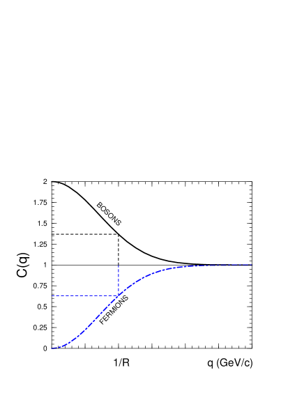
Figure 4: Simple illustration corresponding to the ideal Gaussian source. The upper curve represents to the bosonic case, while the lower curve, the fermionic one. The parameter $R$ is the r.m.s. radius of the emitting region.

To illustrate the correlation function as written in Eq.(9) with a simple analytical example, let us consider the Gaussian profile, i.e.,

$$\rho(x)=e^{-x^{\mu}x_{\mu}/(2R)^{2}}\;\longrightarrow\;\rho(q)=e^{-q^{2}R^{2}/2}\;.$$ (10)

Consequently, in this very simple example, a typical correlation function is written as

$$C(k_{1},k_{2})=1\pm{\bf\lambda}\;e^{-q^{2}R^{2}}.$$ (11)

In equation (11), as we denoted before, the plus sign refers to the bosonic case, and the minus sign to the fermionic one. We easily see that, in this simple example, we would expect experimental ideal HBT data to behave as sketched in Fig. 4, where the upper part refers to bosons and the lower one, to fermions. We see that, in the two-boson (two-fermion) case, there is an enhancement (depletion) of the correlation function in the region where the relative momenta of the pair are small. In both cases of this simple example, the typical size of the emission region corresponds to the inverse width of the $C(k_{1},k_{2})$ curve, plotted as a function of $q=k_{1}-k_{2}$.

Returning to the discussion of the fit parameter $\lambda$, I would like to point out that there is a very simple explanation to reconcile this apparent inconsistency, without the need to introduce this extra degree of freedom. Limited statistics is behind it, since it is virtually impossible to measure two identical particles with exactly the same momenta. This led the experimentalists to split the momenta of the particles in small bins. In more recent times, these bins can be projected in two or more dimensions. For instance, along the income beam direction in fixed target heavy ion collisions ($q_{L}$), and in the direction transverse to it ($q_{T}$). Good quality data allow the experimentalists to consider very small bin sizes. Nevertheless, their range is finite. Being so, when the correlation function is projected along, say, the $q_{T}$ direction, the smallest value of $q_{L}$ is not zero, but within the first (smaller) bin size, in case of high enough statistics. Consequently, we immediately see that the correlation function plotted as a function of $q_{T}$, will not reach the maximum (minimum) value of 2 (0) for bosons (fermions) at $q_{T}=0$. Naturally, the larger the first bin size, the bigger is the deviation from the maximum (minimum) expected value for the correlation function at $q=0$. This can be better seen with the help of Fig. 5, where the two upper curves represent the pure correlation function and the two lower ones, the theoretical correlation functions corrected by the Gamow factor, $\Upsilon(q)$, a multiplicative factor taking into account 2-body Coulomb final state interaction. This factor distorts the pattern, mainly at small values of the momentum difference of the pair, and is written as

$$\Upsilon(q)=\frac{q_{c}/q}{\exp(q_{c}/q)-1}\;\;;\;\;q_{c}=2\pi\alpha m\;,$$ (12)

where $q$ is the four-momentum difference and $\alpha$ is the fine structure constant. The Gamow factor simply multiplies the entire expression in Eq.(9), (11), and all other forms of correlation function for two charged, identical particles. Fig. 5 was generated by the code CERES, whose hypothesis and formulation will be discussed later in this manuscript, in Section II.2.

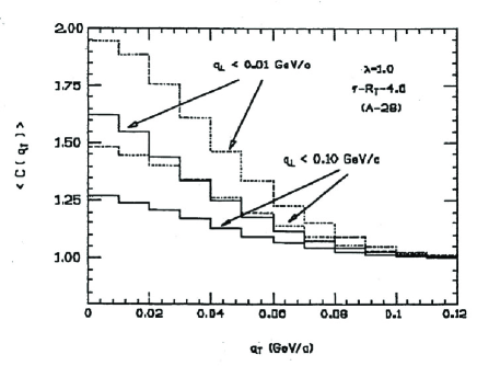
Figure 5: The plot illustrates the fact that we can have the maximum of the bosonic correlation curve below unity, even when the intercept parameter is fixed to be $\lambda=1$. This normally happens in realistic cases of finite statistics. In the plot, we see the two-pion correlation as a function of $q_{T}$, for two possible bin sizes, i.e., for $q_{L}\leq 0.01$ GeV/c and $q_{L}\leq 0.1$ GeV/c. This plot was extracted form Ref.NPA525

We should emphasize, however, that the simple relation between the two-particle correlation function and the Fourier transform of the space-time distribution, as written in Eq. (11) is not straightforward, in general. It is observed only when we can consider the phase-space as decoupled, i.e., $f({\bf x},{\bf p})=\rho({\bf x})g({\bf p})$, where $\rho({\bf x})$ is the source space-time distribution, and $g({\bf p})$ is the energy-momentum distribution. In general, it cannot be decoupled in this way. This is, for example, the case in relativistic heavy ion collisions, where the source expands during its life-time. The reason is that HBT is not only sensitive to the source geometry at particle emission but is also sensitive to the underlying dynamics. This makes the analysis model-dependent and more powerful formalisms (like the one proposed by Wigner, the Covariant Current Ensemble, etc.) must be adopted. We will discuss more about this limitation later on.

I.5 I.5  FURTHER APPLICATIONS

In the 1970’s, Kopylov, Podgoretskiĭ, and Grishinkpg used second-order interferometry to study several interesting problems. For example, they modelled the nucleus as a static sphere with radius R, emitting pions from its surface and got the following correlation function

$$C(k_{1},k_{2})=1\pm[\frac{2J_{1}(q_{T}R)}{q_{T}R}]^{2}[1+(q_{{}_{0}}\tau)^{2}]^{-1}\;,$$ (13)

where

$$q_{\parallel} = {\bf q}.\frac{\bf K}{|\bf K|}$$

$${\bf q_{T}} = {\bf q}-{\bf q_{\parallel}}$$

$$q_{{}_{0}} = E_{1}-E_{2}\approx\frac{1}{2m}({\bf k}^{2}_{1}-{\bf k}^{2}_{2})$$ (14)

$$\approx \frac{1}{2m}({\bf k}_{1}-{\bf k}_{2}).({\bf k}_{1}+{\bf k}_{2})\propto q_{\parallel}\;.$$

The two variables in Eq.(14) are nowadays known as Kopylov variables. With respect to the same parametrization, Cocconicocconi re-interpreted in 1974 the quantity $c\tau=\delta(<R)$ as the thickness of the pion emission layer. They used similar forms for studying: i) the lifetime of excited nuclei through the interferometry of evaporated neutrons, ii) shape and size of multiple production region with $\pi^{\pm}\pi^{\pm}$ correlations, etc. They also applied to CERN/ISR data on $pp,\bar{p}p$.

Many other scientists contributed to the field during that decade. Just to mention a few names, I would quote Shuryak; Biswas; Fowler & Weiner; Giovannini & Veneziano; Grassberger; Yano & Koonin; Gyulassy, Kauffmann & Wilson, etc. Many of these contributions were organized in a collection of reprints, edited by R. M. WeinerWeinerBook , in the late 1990’s, which is a very good source of these reference papers. Among them, the papers by Gyulassy, Kauffmann & WilsonGKW , as well as those by Fowler and Weinerweiner , represented important steps in the field, for introducing more powerful formalisms for studying the cases of coherent, chaotic, and partially coherent sources. On the other hand, Grassbergergrass called the attention to the fact that resonances could play an important role in interferometry, since the long lived ones could distort the correlation function in the region where it was more significant, i.e., at small values of ${\bf q}$, thus changing the chaoticity parameter considerably. This is due to the fact that a resonance of 4-momentum $k$, mass $M$, and width $\Gamma$, would travel a distance $\sim k/(M\Gamma)$ before decaying, causing interference effects whenever $k.q\leq M\Gamma$. The first attempt to analyze the effect of resonances on interferometry in detail was made more than a decade afterwards. I will discuss it later in Sec. II.2.

Despite the comment made earlier in the text, regarding the limitations of the static Gaussian fit, this has always been the preferred source model, due to its simplicity. Along this line, it is instructive to observe that there is a Gaussian limit of Eq.(13), corresponding to

$$[\frac{2J_{1}(q_{T}R)}{q_{T}R}]^{2}\approx e^{-q^{2}_{{}_{T}}R^{2}_{T}/4}\;;\;\frac{1}{[1+(q_{{}_{0}}\tau)^{2}]}\approx e^{-q^{2}_{{}_{0}}\tau^{2}}\;,$$ (15)

a variation of which suggests a non-relativistic parametrization of the correlation function, i.e.,

$$C(k_{1},k_{2})=1\pm{\lambda}\;e^{-q^{2}_{{}_{0}}\tau^{2}/2}e^{-q^{2}_{T}R^{2}_{T}/2}e^{-q^{2}_{L}R^{2}_{L}/2}\;.$$ (16)

The expression in Eq. (16) has been widely employed since the beginning of high energy heavy ion collisions, becoming the standard form to analyze two-particle interferometry, particularly among the experimentalists. In Eq.(16), ${\bf q_{L}}$ is the momentum difference along the direction of the incident beam, ${\bf q_{T}}$ is the component transverse to beam direction, and $q_{{}_{0}}$ is the time component. In the late 80’s, the most popular form changed slightly, according to the suggestion by Bertschbertsch , becoming

$$C(k_{1},k_{2})=1\pm{\lambda}\;e^{-q^{2}_{\small S}R^{2}_{S}}e^{-q^{2}_{\small O}R^{2}_{O}}e^{-q^{2}_{L}R^{2}_{L}/2}\;,$$ (17)

similarly to the previous definition. However, in Bertsch’s suggestion, there was a decomposition of the transverse component, partially incorporating the definition introduced by Kopylov and Podgoretskiĭ, i.e., ${\bf q_{O}}$ and ${\bf q_{S}}$ are both perpendicular to beam direction but ${\bf q_{O}\parallel K_{T}}$ [$=\frac{1}{2}({\bf k_{1_{T}}}+{\bf k_{2_{T}}})$], and ${\bf q_{S}\perp K_{T}}$. As before, ${\bf q_{L}}$ represents the component of the pair momentum difference along the beam direction. Latter, Heinz et al., suggested to include a out-longitudinal cross term in Gaussian fits to the data, i.e., the correlation in this case would be written asheinzchsc

$$C(k_{1},k_{2})=1\pm{\lambda}\;e^{-q^{2}_{\small S}R^{2}_{S}}e^{-q^{2}_{\small O}R^{2}_{O}}e^{-q^{2}_{L}R^{2}_{L}}e^{-2q^{2}_{OL}R^{2}_{OL}}\;.$$ (18)

Ever since, this field has been under constant development and expansion, both in the theoretical and in the experimental grounds. I will briefly highlight only some of the theoretical contributions to the field, mainly focusing at the ones from the Brazilian group and some collaborators from abroad, since a complete discussion of the contribution along theses 50 years is beyond the scope of the present review. For a complete survey of the subject, as well as of the theoretical and experimental progress in the field, I would strongly encourage the reader to look into Refs. WeinerBook ; zajc ; boal ; wong ; heinz1 ; csorgo ; rhic .

II II. CONTRIBUTIONS FROM GROUP MEMBERS

The first contact of the group, whose contributions we are discussing here, with HBT interferometry started in the mid- to late eighties, and was the subject of my PhD ThesisSandraPhD . In fact, it happened a few years before the group itself began performing as a group. Nevertheless, this topic consistently appeared during the group meetings along these years and, since this is a historical perspective, it is worthy to insert the subject in this context. Around the beginning of the decade of 1980, there was already an emerging subject that was attracting the attention of the high energy community: the possible existence of a new state of matter, the Quark-Gluon Plasma (QGP), expected to be produced at high enough temperatures and/or densities. The QGP is a state in which quarks and gluons, the constituents of the hadrons, would be free to wander around a volume much bigger than the usual hadronic size. This state was expected to exist for a brief period of time, since only usual hadrons, with quarks and gluons confined in their interior, have been observed empirically. This imposed the need to look for probes of its existence. Among them, Interferometry was suggested, as a means to estimate the dimensions of the system formed in high energy collisions, thus testing if it was produced in such a new state of matter. In fact, James D. Bjorken was the person who suggested pion interferometry as the subject of my Ph.D. thesisBj83 .

II.1 II.1  EXPANSION EFFECTS IN HBT

In the first paper on the subject, we started by making the hypothesis that the Quark-Gluon Plasma was already being produced in  $pp$ and $\bar{p}p$ collisions at the CERN/ISR. We consideredsandra that the system produced in such collisions expanded before emitting the final particles (hadrons), according to the one-dimensional Landau Hydrodynamical Model Landau . In the initial stage, the system was formed in the QGP phase at a certain temperature, $T_{0}$, started expanding and cooling down, until it reached the critical temperature, $T_{c}$, which we assumed to be of order of pion mass. It could be imagined that, once $T_{c}$ was reached, the hadronization occurred instantaneously, followed by the particle emission. This simplifying hypothesis was actually adopted in the general study of the effects on the correlation function caused by the system expansion. On the other hand, the energy density of the ideal QGP fluid once $T_{c}$ is reached, is much higher that the correspondent one for a hadronic system, due to the statistical degeneracy factors. More explicitly, $\epsilon_{QGP}(T_{c})=\frac{\pi}{30}(g_{g}+\frac{7}{8}g_{q})T_{c}^{4}+B$, where $g_{g}=8(color)\times 2(spin)$, $g_{q}=2(\bar{q}q)\times 3(color)\times 2(spin)\times N_{f}(flavors)$ are the gluon and quark degeneracy factors. The constant $B$ is the vacuum pressure in the MIT Bag model. And, the hadronic correspondent for an ideal gas of pions and kaons, at $T_{c}$, is $\epsilon_{\pi}(T_{c})=\frac{1}{2\pi^{2}}\left[(g_{\pi})\phi(m_{\pi}/T_{c})+g_{K}\phi(m_{K}/T_{c})\right]$, being $g_{\pi}=3$ and $g_{K}=4$, respectively the statistical factor for pions and for kaons (The function $\phi(z)$ is a combination of Bessel modified functions of second class, $K_{i}(z)$, $\phi(z)=z^{2}\sum_{m=0}^{\infty}(\pm 1)^{m}\left\{\frac{3K_{2}[z(1+m)]}{(1+m)^{2}}+z\frac{K_{1}[z(1+m)]}{(1+m)}\right\}$). Nevertheless, the large ratio of the QGP to the hadronic statistical degeneracy factors, together with the entropy conservation during the phase transition, make the duration of the mixed phase very long. And mesons would be emitted during all that period. This was a more realistic hypothesis that was adopted when comparing our predictions with experimental data. However, for the sake of simplicity, we considered in the calculation that the emission occurred at a typical average freeze-out time, $<\tau_{f}>$.

In our calculation, we neglected the transverse expansion and used the asymptotic Khalatnikov solution, i.e.

$$\xi \equiv \ln\left(\frac{T}{T_{0}}\right)\simeq-c_{0}^{2}\ln\left(\frac{\tau}{\Delta}\right)$$

$$\alpha \simeq \frac{1}{2}\ln\left(\frac{t+x}{t-x}\right)$$ (19)

where $\alpha$ is the system rapidity, $c_{0}\approx 1/\sqrt{3}$ is the sound velocity $\sqrt{(1-c_{0}^{2})/\pi l}$, being $l$ the initial thickness of the fireball (solution valid whenever $\xi\gg|\alpha|$). This is essentially the Bjorken picture of hydrodynamics but with different initial conditions. In the version we adopted of the hydrodynamics, the initial temperature $T_{0}$ depends on the value of the fireball, with mass $M$, initially formed in high energy hadronic collisions. The hypothesis we used was that a large Lorentz-contracted fireball was formed around one of the incident particleshama , constituted of quarks and gluons, with initial radius $R\simeq R_{proton}$. The fireball mass was estimated as the missing mass, i.e., by discounting the fraction of the energy available in the center of mass of the $\bar{p}(p)p$ collision that was dragged by the dominant particle after the collision happened. For relating this initial temperature with the fireball mass, we equated the number of produced hadrons at $T_{c}$ to the (conserved) entropy, which can easily be estimated for a QGP as $S(T_{0})=s(T_{0})V_{QGP}$. The initial volume of the QGP can be related to the initial energy density, $\epsilon_{0}$, which can be simply written as $\epsilon_{0}=M/V_{QGP}$. The initial entropy density, $s(T_{0})$, can be estimated through statistical relations, leaving the calculation of the initial QGP volume to be made. Since we considered $\bar{p}(p)p$ collisions, we assumed that $V_{QGP}=\frac{4}{3}\pi R_{0}^{3}\frac{2m_{p}}{M}$, where $R_{0}$ and $m_{p}$ are, respectively, the proton radius and mass. At the end, the final proportionality coefficients were estimated with the help of the experimental data on charged multiplicity versus the missing mass. Finally, the initial temperature was related to the fireball mass by a numerical factor, $T_{0}=0.0989\sqrt{M}$. From that, we estimated $\tau_{c}$, instant corresponding to the beginning of the phase transition, $\tau_{c}=\Delta\left(\frac{T_{0}}{T_{c}}\right)$, and also the instant it ended, $\tau_{f}$, as well as the typical (average) duration, $<\tau_{f}>$ (see Ref. sandra for details).

We had adopted the Kopylov variables described before, in Eq. (14) and sketched in Fig. 6, as the relevant momentum difference of the pair of pions.

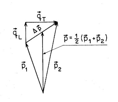
Figure 6: Illustration of the Kopylov variables: we see that $\vec{q_{L}}\equiv\vec{q_{\parallel}}\parallel\vec{K}$ and $\vec{q_{T}}\equiv\vec{q_{\perp}}\perp\vec{K}$. The figure also shows other notations commonly used: $\vec{q}\equiv\vec{\Delta p}$ and $\vec{K}\equiv\vec{p}$.

For studying the general behavior of the correlation function under the influence of the expansion effects, we assumed that each point on the surface $\tau=\tau_{f}$ of the QGP, where $T=T_{c}\simeq m_{\pi}$, was an independent chaotic source with momentum spectrum given by

$$f(p)\simeq\frac{1}{(2\pi)^{3}}\frac{u^{\mu}p_{\mu}}{E}\exp{(-\frac{u^{\mu}p_{\mu}}{T_{c}})}\;,$$ (20)

where $u^{\mu}=(\cosh\alpha,\sinh\alpha,0,0)$ is the 4-velocity of the fluid, and $p^{\mu}=(E,p_{x},p_{y},p_{z})$ is the 4-momentum of the emitted particle. The amplitude for a particle emitted at $x^{\prime}$ to be observed at $x$ is written as

$$A(x,x^{\prime})=\int d{\vec{p}}\sqrt{f(p)}\exp{[-ip_{\mu}(x^{\mu}-x^{\prime\mu})]}e^{i\phi(x^{\prime})}\;,$$ (21)

where $\phi(x^{\prime})$ is a random phase. We followed the formulation and notation of Ref.shuryak for writing the probability of detecting two quanta of momenta $p_{1}$ and $p_{2}$ in an event, as

$$W(p_{1},p_{2})=\tilde{I}(0,p_{1})\tilde{I}(0,p_{2})+|\tilde{I}[(p_{1}-p_{2}),\frac{1}{2}(p_{1}+p_{2})]|^{2}\;,$$ (22)

where

$$\tilde{I}[(\Delta p),p]\!=\!\int dx\;d(\Delta x)e^{i(x\;\Delta p+\Delta x\;p)}\int dx^{\prime}I(x,\Delta x,x^{\prime})\;,$$ (23)

and

$$\langle A^{*}[x-\frac{\Delta x}{2},x^{\prime}]A^{*}[x+\frac{\Delta x}{2},x^{\prime}]\rangle=\delta(x^{\prime}-x)I(x,\Delta x,x^{\prime})\;.$$ (24)

The average indicated in the above equation is taken over the random phases $\phi(x^{\prime})$ and $\phi(x^{\prime\prime})$. In particular, we see that the single-inclusive distribution is written as

$$W(p_{i})=\langle|\int dx^{\prime}\int dxe^{ip_{i}.x}A(x,x^{\prime})dx|^{2}\rangle=\tilde{I}[0,p_{i}]\;,$$ (25)

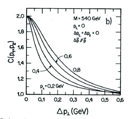
Figure 7: $C(p_{1},p_{2})$ as a function of the momentum difference $\Delta p_{T}$ ($\equiv q_{T}$, in the text), for several values of the average momentum $p_{\perp}$ ($\equiv K_{T}$ in the text). A clear dependence is seen: the curves broaden with increasing average momentum, showing a progressively smaller effective emission region. This plot is a reproduction of the one originally published in Ref.sandra .

From this formulation we obtained the expression for the two-particle correlation function. With that, we studied several different kinematical zones, trying to apprehend the lessons that idealized theoretical cuts could teach us. Many interesting and important results came out of that study (see Ref. sandra for details).

The first, unexpected effect, was showing a clear influence of different emission times at which the pions were emitted from the source. I will write it in a simple analytical form, later in the text. This effect showed itself into the correlation function when plotted as a function of $q_{T}$, the Kopylov variable parallel to the average momentum of the pair, ${\bf K}=\frac{1}{2}({\bf k_{1}}+{\bf k_{2}})$. It is illustrated in Fig. 7. Independently of our knowledge, S. Pratt had also suggested that the time would influence the correlation function, so that large short-lived sources could result into a similar correlation function as a short long-lived one pratt .

The dependence on the average momentum of the pair, ${\bf K_{T}}$, shown above, was a symptom of effects coming from the underlying dynamics, and reflected the break-up of the naive picture, in which the correlation function depended exclusively on the variable ${\bf q_{T}}$, as in the Gaussian example discussed above.

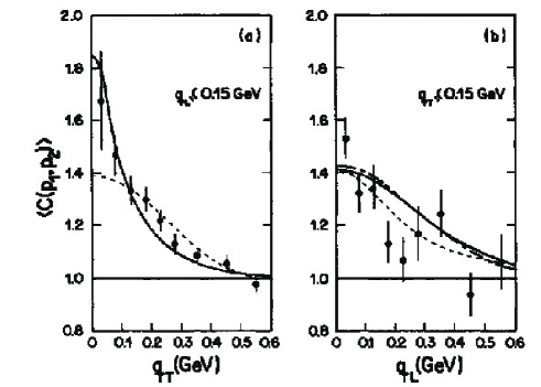
Figure 8: In (a), the two-pion correlation function is shown in as a function of the Kopylov variable $q_{T}$, averaged over the interval $q_{L}\leq 0.15$ GeV (we adopted natural units, in which $\hbar=c=1$). In (b), it is shown as a function of the other component, ${\bf q_{L}}\parallel{\bf K}$, for $q_{T}\leq 0.15$ GeV. The data points are from Ref. israfs . These plots were originally published in Ref.sandra .

We also compared our results with data of $pp$ and $\bar{p}p$ collisions at CERN/ISR ($\sqrt{s}=53$ GeV) and could efficiently describe the trend of data. This was maybe the only successful description of that particular experimental result, reflecting the need for more powerful formalisms when describing HBT interferometry at high energies. In this case, in an effort to make the estimate more realistic, we considered that the emission occurred later, at a typical instant of time $<\tau_{f}>$, averaged over the long period that lasted the first order phase transition. We should notice that the curves in Fig. 8 are not fits, but predictions from the model, obtained without the need for introducing the $\lambda$ parameter (which is equivalent to fixing $\lambda=1$). Similar treatment within the same model was also given to two-kaon interferometry data from the same experimentsandra , successfully describing data.

Fig. 7 and 8 above also show another important result from that study: the observation of strong distortions in the correlation function, definitely departing from the Gaussian shape, due to the dynamical effects related to the expansion of the system.

II.2 II.2  NON-IDEAL EFFECTS

More than 10 years after Grassberger pointed out the important role resonances could have in interferometry we investigated it in detail, in collaboration with M. Gyulassygyupad89 . In particular, we analyzed the effect of resonances decaying into pions, following the predictions of resonance fractions from the ATTILA version of the Lund modelatt . Very briefly, it can be understood as follows: long lived resonances, such as $\omega$, $\eta$, $\eta^{\prime}$, can mimic sources with longer life-times, even if they freeze-out simultaneously as the direct $\pi$’s.

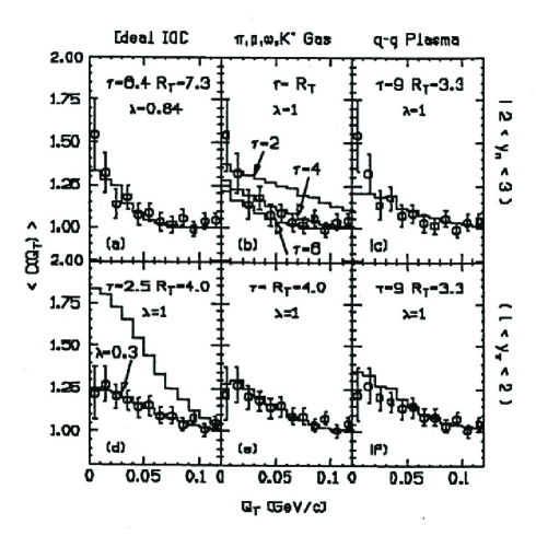
Figure 9: The two-pion correlation function is shown in three different scenarios, as a function of $q_{T}$. The first, in parts (a) and (d) were calculated assuming an ideal inside-outside cascade source (IOC) as in the 1-D Bjorken pictureBj . In parts (b) and (e), a non-ideal resonance gas source is considered with parameters suggested by the ATTILA version of the Lund model. Parts (c) and (f) correspond to the QGP model of Ref.gb . Plots in the upper panel were calculated in the central rapidity region ($2<y_{\pi}<3$), whereas the ones in the lower panel refer to $1<y{{}_{\pi}}<2$. This figure is a reproduction of the one originally published in Ref.gyupad89 .

I call the attention to the fact that, although denoted by the same letters, the variables $q_{L}$ and $q_{T}$ of momentum difference, appearing in Fig. 9, are defined as the components parallel and perpendicular to the incident beam direction, respectively, as became a convention in high energy heavy ion collisions.

It was very important to verify if we could explain the preliminary results obtained by the NA35 collaboration (CERN/SPS)NA35 colliding O+Au at 200 GeV/nuclear in a more conventional way, without assuming QGP formation. This last hypothesis had been suggested by G. Bertschgb at that time as the only possible explanation. Actually, by introducing resonances decaying into pions explicitly into interferometry, we managed to demonstrate that our result, assuming the formation of a regular hadronic system and no QGP, led to an equally good agreement with data, as can be seen from Fig. 9. In fact, we showed in Ref. gyupad89 (and presented in the Quark matter ’88 Conference qm88 ) that the NA35 preliminary data of that time was consistent with a wider range of pion source parameters when additional non-ideal dynamical and geometrical degrees of freedom were incorporated into the analysis by extending the Covariant Current FormalismGKW ; gyupad89 ; KG .

II.3 II.2.1  Ideal Bjorken IOC Picture

In the Covariant Current Ensemble formalismgyupad89 ; GKW ; KG , the correlation function for identical bosons (since mainly bosonic HBT will be discussed in this review) can be expressed as

$$C(k_{1},k_{2})=C(q,K)=1+\lambda\frac{|G(q,K)|^{2}}{G(k_{1},k_{1})G(k_{2},k_{2})}\;\;,$$ (26)

where $q^{\mu}=k_{1}^{\mu}-k_{2}^{\mu}$ and $K^{\mu}=\frac{1}{2}(k_{1}^{\mu}+k_{2}^{\mu})$.

The complex amplitude, $G(k_{1},k_{2})$, can be written as

$$G(k_{1},k_{2})=\int d^{4}xd^{4}p\;e^{iq^{\mu}x_{\mu}}D(x,p)j_{0}^{*}(u_{f}^{\mu}k_{1\mu})j_{0}(u_{f}^{\mu}k_{2\mu})\;\;,$$ (27)

where $D(x,p)$ is the break-up phase-space distributiongyupad89 ; pg:nioc and the currents, $j_{0}(u_{f}.k_{i})$, contain information about the production dynamics. The one-particle spectrum is obtained from Eq. (27) by imposing $k_{1}=k_{2}$, which leads to

$$G(k_{i},k_{i})=\int d^{4}xd^{4}p\;D(x,p)|j_{0}(u_{f}^{\mu}k_{i\mu})|^{2}\;\;.$$ (28)

The currents $j_{0}(u_{f}.k_{i})$ in Eqs. (27,28) can be associated to thermal models, and can be written in a covariant way as

$$j_{0}(k)\propto\sqrt{u^{\mu}k_{\mu}}\exp{\{-\frac{u^{\mu}k_{\mu}}{2T}\}}\;.$$ (29)

However, to make the computation easier, we adopted a more convenient parametrization

$$j_{0}(u.k)=\exp{\{-\frac{u^{\mu}k_{\mu}}{2T_{ps}}\}}\;\;,$$ (30)

where the so-called pseudo-temperature $T_{ps}$ is related with the true temperature $T$ according toKG

$$T_{ps}(x)=1.42T(x)-12.7\text{ MeV}\;.$$ (31)

This mapping between $T(x)$ and $T_{ps}(x)$ was later shown to be a good approximation also in the case of kaon interferometrypadrol .

With the covariant pseudo-thermal parametrization as in Eq. (30), the complex amplitude can be rewritten in a simpler form,

$$G(k_{1},k_{2})=\langle e^{iqx_{af}}e^{-Kp_{af}/(mT)}\rangle\;\;,$$ (32)

where the bracket $<...>$ denote an average over the pion freeze-out phase-space coordinates.

In the case of Bjorken ideal Inside-Outside Cascade (IOC) picture, the phase-space distribution involves a fixed freeze-out proper time $\tau_{f}$ and a perfect correlation between $\eta$ and $y$. The correspondent phase-space distribution is written as

$$D(x,p)=\frac{1}{E_{f}}\rho\frac{1}{\tau_{f}}\delta(\tau_{f}-\tau)\delta(\eta-y)\delta(p_{0}-E_{\bf p})g({\bf p}_{T})\frac{e^{\frac{-x_{T}^{2}}{R_{T}^{2}}}}{\pi R_{T}^{2}}\;,$$ (33)

where $E_{\bf p}={\sqrt{{\bf p}^{2}+m^{2}}}$ is the energy and $g({\bf p}_{T})$ is the transverse momentum distribution; the rapidity distribution is considered to be uniform, i.e., $\frac{dN}{dy}=\rho$. In the ideal IOC picture, there is a perfect correlation in phase-space between the space-time rapidity

$$\eta=\frac{1}{2}\ln[\frac{t+z}{t-z}]$$ (34)

and the energy-momentum rapidity,

$$y=\frac{1}{2}\ln[\frac{E+p_{z}}{E-p_{z}}]\;,$$ (35)

i.e., they are indistinguishable.

To obtain simple analytical equations, we assume a very narrow distribution of ${\bf p}_{T}$ around small momenta, i.e., $g({\bf p}_{T})=\delta^{2}({\bf p}_{T})$. The finite pion wave-packets generate the finite $p_{T}$ distribution in our case. By substituting $D(x,p)$ from (33) into (27) and considering the pseudo-thermal parametrization (30) for the currents, the function $G(k_{1},k_{2})$ was found to beKG

$$G(k_{1},k_{2})=2<\frac{dN}{dy}>\{\frac{2}{q_{T}R_{T}}J_{1}(q_{T}R_{T})\}K_{0}(\xi)\;\;,$$ (36)

where

$$\xi^{2} = [\frac{1}{2T_{ps}}(m_{1T}+m_{2T})-i\tau(m_{1T}-m_{2T})]^{2}+$$ (37)

$$2(\frac{1}{4T_{ps}^{2}}+\tau^{2})m_{1T}m_{2T}[\cosh(\Delta y)-1]\;\;,$$

and $\Delta y=y_{1}-y_{2}$.

The single-inclusive distribution is then written as

$$G(k_{i},k_{i})=E\frac{d^{3}N}{dk_{i}^{3}}=2<\frac{dN}{dy_{i}}>K_{0}(\frac{m_{i_{T}}}{T_{ps}})\;.$$ (38)

To compare theoretical correlation functions with data projected onto two of the six dimensions, we computed the projected correlation function trying to mimic what is done in the experiment, i.e.,

$$C_{\!proj}(q_{T},q_{L})\!=\!\!\!\frac{\int d^{3}k_{1}d^{3}k_{2}P_{2}({\vec{k}}_{1},{\vec{k}}_{2})A_{2}(q_{T},q_{L};{\vec{k}}_{1},{\vec{k}}_{2})}{\int d^{3}k_{1}d^{3}k_{2}P_{1}({\vec{k}}_{1})P_{1}({\vec{k}}_{2})A_{2}(q_{T},q_{L};{\vec{k}}_{1},{\vec{k}}_{2})}\;,$$ (39)

where $P_{1}$ and $P_{2}$ are, respectively, the single- and two-pion inclusive distributions. It is essential to have perfect correspondence between the experimental information and the theoretical estimates concerning the number of dimensions into which the correlation data is projected, the cuts in momentum and rapidity, the sizes of the bins, etc. $A_{2}$ is the experimental two-particle binning and acceptance function, through which we approximate the theoretical estimate to the empirical cuts.

We should notice that, experimentally, the two-particle correlation function in high energy collisions is obtained by measuring the following ratio

$$C_{exp}(i,j) = {\cal N}_{exp}\times\frac{A(i,j)}{B(i,j)}$$

$$\Delta C_{exp}(i,j) = C_{exp}(i,j)\sqrt{\left[\frac{\Delta A(i,j)}{A(i,j)}\right]^{2}+\left[\frac{\Delta B(i,j)}{B(i,j)}\right]^{2}}$$

$$\;\;.$$ (40)

The numerator $A(i,j)\pm\Delta A(i,j)$ corresponds to the combination of pairs of identical particles from the same event, and the denominator, $B(i,j)\pm\Delta B(i,j)$, represents the background; ${\cal N}_{exp}$ is an experimental normalization. Historically, the background for identically charged pions have been the combination of unequally charged ones. However, later it was realized that $\pi^{+}\pi^{-}$ could frequently come from the decay of resonances, which would distort the background and cause strange pattern for the correlation function built in this way. They soon realized that a better way to construct the background was to combine identically charged particles, but from different events. Another possibility used sometimes is a Monte Carlo simulated background, taking into account the experimental cuts and acceptance.

II.4 II.2.2  Non-ideal IOC

The non-ideal picture mentioned before referred to the underlying effects that would be important to incorporated into the interferometric analysis, even restricting the attention to completely chaotic sources. For instance, the $\pi^{-}$ rapidity distribution at 200 AGeV was clearly not uniform, as assumed in the asymptotic Bjorken picture, but would be better described by a Gaussian with width $Y_{c}\approx 1.4$NA35 . On the other hand, a large fraction of the pions could arise from the decay of long lived resonances, such as $\omega$, $K^{*}$, $\eta$, etc, as was suggested by Grassbergergrass . In coordinate space, the finite nuclear thickness, together with resonance effects, could lead to a large spread ($\Delta\tau$) of the freeze-out proper times, and to a wide distribution of transverse decoupling radii ($R_{T}$). In phase-space, there is not the perfect correlation between the space-time and energy-momentum rapidity variables present in the ideal Bjorken picture. Instead, as suggested by the ATTILA version of the Lund model, they would be better related by a Gaussian with finite width $\Delta\eta$. Besides, other correlations may have to be considered if collective hydrodynamic flow occurs, for instance, between transverse coordinates (${\vec{x}}_{\perp}$) and transverse momentum component (${\vec{p}}_{\perp}$). All these effects together were generically called as the non-ideal picture, which is equivalent to considering a more realistic picture than the one idealized by the Bjorken in his version of the 1-D hydrodynamics. The phase-space distribution representing these effects together can be obtained from Eq. (33) by replacing

$$\rho\frac{1}{\tau_{f}}\delta(\tau_{f}-\tau)\delta(\eta-y)\rightarrow\frac{2}{\Delta\tau^{2}}\exp\left(\frac{-\tau_{f}^{2}}{\Delta\tau^{2}}\right)\times$$

$$\exp\left[-\frac{(y-y^{*})^{2}}{2Y_{c}^{2}}\right]\frac{1}{\sqrt{2\pi}\Delta\eta}\exp\left[-\frac{(\eta-y)^{2}}{2\Delta\eta^{2}}\right]\;.$$ (41)

Besides the modification in Eq.(41), there is a major correction to be added, i.e., the effect of long-lived resonances decaying into pions. This can be included in the semiclassical approximationqm88 ; gyupad89 . The pion freeze-out coordinates, $x_{a}^{\mu}$, can be related to the parent resonance production coordinates, $x_{r}^{\mu}$, through

$$x_{a}^{\mu}=x_{r}^{\mu}+u_{r}^{\mu}\tau\;\;,$$ (42)

where $u_{r}^{\mu}$ is the resonance four velocity and $\tau$ is the proper time of its decay. Summing over resonances $r$ of widths $\Gamma_{r}$, and averaging over their decay proper times, we obtain, instead of Eq.(32) the final expressionqm88 ; gyupad89

$$G(k_{1},k_{2})\approx\langle\;\sum_{r}f_{\pi^{-}/r}\frac{\exp(iqx_{r}-Ku_{r}/T_{r})}{\left(1-iqu_{r}/\Gamma_{r}\right)}\;\rangle\;\;,$$ (43)

where $f_{(\pi^{-}/r)}$ is the fraction of the observed $\pi^{-}$’s arising from the decay of a resonance of type $r$, and the temperature $T_{r}$ characterizes the decay distribution of that resonance. According to the Lund model, the main resonance contributing to the negative pion yield at CERN/SPS energies are $f_{(\pi^{-}/\omega)}=0.16$, $f_{(\pi^{-}/K^{*})}=f_{[\pi^{-}/(\eta+\eta^{\prime})]}=0.09$, $f_{(\pi^{-}/\rho)}=0.40$, $f_{(\pi^{-}/direct)}=0.19$. Although we included direct pions and the ones coming from $\rho$ decay independently, they are hardly distinguishable, since $\rho$’s decay very fast.

All these effects combined were simulated in a Monte Carlo code, named CERES, which was also able to include simplified subroutines which mimicked the experimental cuts and acceptancegyupad89 ; qm88 ; pg:nioc .

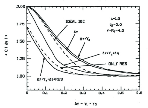
Figure 10: Numerical results for the pion correlation function versus $\Delta y$ are shown in the central rapidity region, when the non-ideal effects are introduced, one by one. This plot is a reproduction of the one originally published in Ref.pg:nioc .

For explicitly demonstrating how the above results would show themselves into the correlation function, we derived in Ref. pg:nioc several analytical relations where the non-ideal effects were progressively introduced. We started with the ideal Bjorken 1-D picture. Then, instead of the instant freeze-out assumed there, we considered a spread ($\Delta\tau$) and, subsequently, all the other effects mentioned above, one by one. For fixed $q_{T}=0$, the results as a function of the rapidity difference $\Delta y$ ($\approx q_{L}/m_{T}$ for $\Delta y\ll 1$), can be seen in Fig. 10. For generating these plots, we estimated the correlation function using the code CERES and adopting the following values for the parameters: $R_{T}\approx 4$fm, $\tau_{f}\approx 4$fm/c, fixed the intercept parameter $\lambda=1$, $\Delta\tau=4$ fm/c; $Y_{c}\approx 1.4$, $\Delta\eta\approx 0.8$, plus the above fractions $f_{\pi/r}$ from the Lund model, when adding resonances.

In the curves shown in Fig. 9, nevertheless, we had three sets of parameters, corresponding to the different models compared there: in the Lund resonance case, besides the fractions $f_{\pi/r}$, we used $Y_{c}\approx 1.4$, $\Delta\eta\approx 0.7$, $R_{T}\approx 3$fm, $\tau_{f}\approx 3$fm/c, $y^{*}=2.5$ and fixed $\lambda=1$; for mimicking the QGP model of Ref.gb , we used no resonance, $\tau_{f}=9.0$ fm/c, $R_{T}=3.3$ fm, $\Delta\eta\approx 0.76$, assuming $Y_{c}\rightarrow\infty$ and $\lambda=1$.

The results shown previously in Fig. 9 clearly posed another problem to the interferometric probes of high energy heavy ion collisions: several very distinct dynamical scenarios could lead to approximately the same final correlation function and similar experimental HBT results.

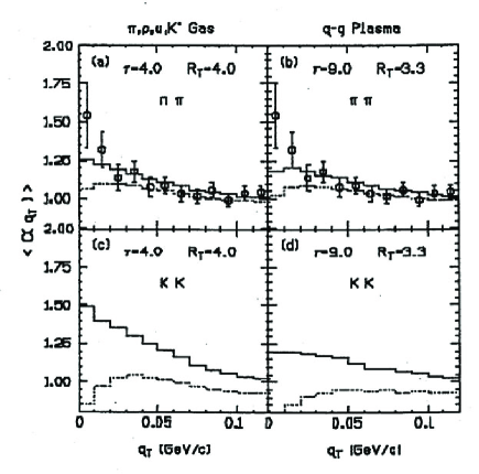
Figure 11: Comparison of two-pion, in parts (a) and (b), and two-kaon projected correlation functions, in parts (c) and (d) is considered as a function of the transverse momentum difference, $q_{T}$. The plots are calculated in the central rapidity region and with $q_{L}\leq 0.1$ GeV. Solid (dashed) lines indicate correlations without (with) Coulomb distortions. Parts (a) and (c) correspond to predictions based on the Lund modelatt , and parts (b) and (d), to the plasma hydrodynamical model of Ref.gb . The pion data is from Ref.NA35 . This figure was extracted from Ref.gyupad89a .

One possibility to discriminate among very different scenarios, suggested in Ref. gyupad89a , was to explore distinct freeze-out geometries by comparing pion and kaon interferometry. This suggestion was motivated by the fact that an entirely different set of hadronic resonances decay into pions than into kaons. In the first case, according to the ATTILA version of the Lund fragmentation model, long lived resonances such as $\omega$, $\eta$ and $\eta^{\prime}$, contribute to the final pion yield, whereas, in the second case, half of the kaons are produced by direct string decay, and the other half by the decay of $K^{*}$. On the other hand, in the QGP model considered previously in Ref.gyupad89 for comparison, the freeze-out geometry of all hadrons was expected to be about the same. In the case of pions, we saw from Fig. 9 that both cases led to equally good results as compared to the experimental points. In the case of kaons, then, an entirely different behavior would be expected. Indeed, we see from Fig. 11 a more significant difference between those two models, helping to separate long-lived scenarios from those where HBT results were generated by the effect of resonances.

The important role of resonances stressed above led us to investigate how would be their influence for much smaller systems at higher energies. For this, we looked into $\bar{p}p$ and $pp$ data from CERN/ISRlorstad . For simplicity, in this calculation, we assumed the ideal Bjorken picture to describe the freeze-out distribution. Surprisingly, the resultnpa544 turned out to be neither compatible with the absence of resonance nor with the full resonance fractions predicted by the Lund fragmentation model mentioned before. Instead, the data seemed to be best described by the scenario with about half the resonance fractions predicted by the Lund model, as can be seen in Fig.12.

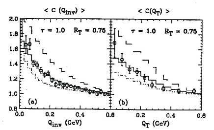
Figure 12: Negative pion correlation in $\bar{p}p$ and $pp$ reactions at CERN/ISR energies are shown as a function of $Q_{inv}$ on the left plot, and as function of $q_{T}$ (with $q_{L}\leq 0.15$ GeV/c) on the right plot. Dashed, solid and dot-dashed histograms indicate the calculated correlation functions with, respectively, no, half and full Lund resonance abundances. The data points are from Ref.lorstad on the left, and from Ref. israfs , on the right hand side. Both plots were extracted from Ref.NPA525 .

Meanwhile, we also derived a general and powerful formulationpgg , based on the Wigner density formalism, which allows to treat complex system, by including an arbitrary phase-space distribution (i.e., the momentum distribution, $g({\bf p})$, and the space-time one, $\rho({\bf x})$, could be entangled) and multi-particle correlations. This formalism corresponds to a semiclassical generalization of the n-particle phase-space distribution, in which it is allowed for a Gaussian spread of the coordinates around the classical trajectories, in order to incorporate minimal effects due to the uncertainty principle. Also, correction terms due to pion cascading before freeze-out were derived using this semi-classical hadronic transport model. Such terms, however, can be neglected if the mean free path of pions is small compared to the source size, or if the momentum transfers are small compared to the pion momenta. The main result of that investigation can be summarized by the following formula for the Bose-Einstein symmetrized n-pion invariant distribution

$$P_{n}({\bf k_{1}},...,{\bf k_{n}}) \propto \;\langle\sum_{\sigma}\prod_{j=1}^{n}\exp\left[i(k_{j}-k_{\sigma_{j}}).x_{j}\right]$$ (44)

$$\;\;\;\;\;\tilde{\delta}_{\Delta}(k_{j}-k_{\sigma_{j}},p_{j})\;\rangle\;,$$

with the smoothed delta function given by

$$\tilde{\delta}_{\Delta}(k-k^{\prime},p-K) = \frac{\!\exp\{[p-\frac{1}{2}(k+k^{\prime})]^{2}/(2\Delta p^{2})\}}{{(2\pi\Delta p^{2})}^{\!-3/2}}$$ (45)

$$\times\;\;\exp[\frac{\Delta x^{2}}{2}(k-k^{\prime})^{2}]\;.$$

The brackets $<...>$ denote an average over the $8n$ pion freeze-out coordinates $\{x_{1},p_{1},...,x_{n},p_{n}\}$, as obtained form the output of a specific transport model, such as a cascadegb or the Lund hadronization modelatt . In the form written in Eq. (44) and (45), this formulation is ideally suited for Monte Carlo computation of pion interference effects. The smoothed delta function results from the use of Gaussian wave packets with widths $\Delta x$ and $\Delta p$, which depend on details of the pion production mechanism. The sum runs over $n!$ permutations $\sigma=(\sigma_{1},...,\sigma_{n})$ of the indices; $x,k,p,...$ denote 4-vectors and all momenta are on-shell. This is a generalization of the Wigner type of formulation proposed in Ref.shuryak and used in the pioneer work of HBT in the group, discussed in Section II.1 and in Ref. SandraPhD ; sandra . As a special limit, we found out that, for minimum Gaussian packets, i.e., $\Delta x\Delta p=1/2$, having $\Delta p\simeq mT_{ps}$, where $m$ is the particle mass and $T_{ps}$ is the pseudo temperature of Eq. (31) we recovered the interferometric relations derived within the Covariant Current Ensemble formalismGKW , which, for the sake of simplicity, was adopted as a first approach to the study of non-ideal effects on Interferometry described above.

An equivalent alternative way of expressing Eq.(44) is pgg

$$P_{n}({\bf k_{1}},...,{\bf k_{n}})\approx\;\langle C_{N,n}\rangle\sum_{\sigma}\prod_{j=1}^{n}D_{\Delta}[q(j,\sigma_{j}),{\vec{K}}(j,\sigma_{j})]\;,$$ (46)

with

$$D_{\Delta}(q,{\vec{K}})=\int d^{4}x\int d^{3}p\;e^{iqx}D(x,{\vec{p}})\tilde{\delta}_{\Delta}(q,p-K),$$ (47)

where $D(x,{\vec{p}})$ can be given by, for example, Eq.(33), and $C_{N,n}\equiv N!/(N-n)!$, where $n=2$ in case of two-pion correlations, and $N$ is the multiplicity of the event.

An interesting simple point explicitly demonstrated in Ref. pgg , is the dependence of the effective transverse radius on the average momentum of the pair, which was already shown in Fig.7, as one of the results of Ref.sandra , and also suggested in pratt . This dependence on $K_{T}$ appears through the time dependence of the emission process. The demonstration was done by means of a simple Gaussian example, as in Eq. (16). For better understanding it, we should recall the definition of the average 4-momentum of the pair, $K^{\mu}$, and their difference, $q^{\mu}$, i.e.,

$$q^{\mu}=(k^{\mu}_{1}-k^{\mu}_{2})\;;\;K^{\mu}=\frac{1}{2}(k^{\mu}_{1}+k^{\mu}_{2})\;.$$ (48)

From the above relations, it immediately follows that

$$q^{\mu}K_{\mu}=q^{0}K_{0}-{\bf q.K}\equiv 0\rightarrow q^{0}=\frac{{\bf q.K}}{E_{K}}=\frac{{\bf q_{T}.K_{T}}+q_{L}K_{L}}{E_{K}}\;,$$ (49)

where $E_{K}=\sqrt{{\bf K}^{2}+m^{2}}$ was written for the sake of simplicity.

Propagating the above result into the Gaussian correlation function, we get

$$R^{2}_{T_{\small eff}} \approx 2R_{T}^{2}+(\Delta\tau)^{2}({\bf K}^{2}_{T}/E_{K}^{2})$$

$$R^{2}_{L_{\small eff}} \approx R_{L}^{2}+(\Delta\tau)^{2}(K^{2}_{L}/E_{K}^{2})\;.$$ (50)

The results on Eq. (50) show that the time spread of the source freeze-out generally enhances the effective size measured by interferometry.

I should remark that several contributions and invited talks presented in international conferences in the period are being omitted here, due to the lack of space. I would address to the Quark Matter Conference proceedings for that, as well as the proceedings of the RANP Conference and of Hadron Physics.

II.5 II.3  DISCRIMINATING DIFFERENT DYNAMICAL SCENARIOS

The coincidental agreement with data of two opposite scenarios, such as the resonance gas and the QGP discussed before, in Fig. 9, stressed the necessity of finding other means to more clearly discriminate among different decoupling geometries. Although the comparison of kaon with pion interferometry was shown to be helpful, as seen in Fig. 11, it still lacked from more quantitative information. Then, how to disentangle different models in a more precise way?

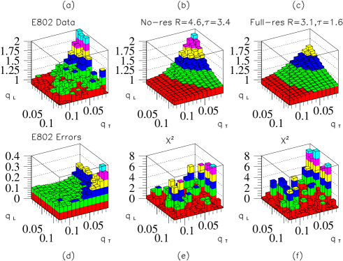
Figure 13: $\pi^{-}\pi^{-}$ correlations in central Si+Au collisions is shown as a function of $q_{T}$ and $q_{L}$. The preliminary E802 datae802 corrected for acceptance and Coulomb effects are shown in part (a). Parts (b) and (c) show theoretical correlation functions filtered with the E802 acceptance. They correspond, respectively, to cases without and with resonance production. This figure was extracted from Ref.PLB348 .

In order to answer this question, M. Gyulassy and myself developed a method, in which a 2-D $\chi^{2}$ analysis was performed, comparing two-dimensional theoretical and experimental pion interferometry resultsPLB348 . For illustrating the method we performed the calculations using the code CERES mentioned above, for two very distinct scenarios. The first one considered the effects of resonances decaying into pions, including Lund resonance fractions. The other one ignored the contribution of resonances. The data points were kindly sent to us by Richard Morse, from the BNL/E802 Collaboration, and corresponded to $Si+Au$ collisions at 14.6 GeV/ce802 , as measured at the BNL/AGS. I will summarize the method by recalling Eq. (39) and Eq. (40). The E802 experimental acceptance functions for two particles was approximated by

$$\!\!A_{2}(q_{T},q_{L};{\vec{k}}_{1},{\vec{k}}_{2})=A_{1}({\vec{k}}_{1})A_{1}({\vec{k}}_{2})\Theta(20-|\phi_{1}-\phi_{2}|)$$ (51)

$$\;\;\;\;\;\;\;\;\;\delta(q_{L}-|k_{z1}-k_{z2}|)\delta(q_{T}-|{\vec{k}}_{T_{1}}-{\vec{k}}_{T_{2}}|)\;\;.$$

The angles are measured in degrees and the momenta in GeV/c. The single-inclusive distribution cuts were specified by

$$A_{1}({\vec{k}}) = \Theta(14<\theta_{lab}<28)$$ (52)

$$\Theta(p_{lab}<2.2\;{\rm GeV/c})\Theta(y_{min}>1.5)\;\;.$$

The input temperature matching the experimentally observed pion spectrum was $T\approx 170$ MeV.

For the purpose of performing a quantitative analysis of the compatibility of different scenarios with data, we computed the $\chi^{2}$ goodness of fit on a two-dimensional grid in the $(q_{T},q_{L})$ plane, binned with $\delta q_{T}=\delta q_{L}=0.01$ GeV/c. The $\chi^{2}$ variable was computed (as suggested by W. A. Zajc) through the following relationPLB348

$$\chi^{2}(i,j)=\frac{[A(i,j)-{\cal N_{\chi}}^{-1}C_{th}(i,j)B(i,j)]^{2}}{\{[\Delta A(i,j)]^{2}+[{\cal N_{\chi}}^{-1}C_{th}(i,j)\Delta B(i,j)]^{2}\}}\;\;,$$ (53)

where ${\cal N}_{\chi}$ is a normalization factor estimated as to minimize the average $\chi^{2}$, which depends on the range in the $q_{T},q_{L}$ plane under analysis. The minimization of the average $\chi^{2}$ was performed by exploring the parameter space of the transverse radius $R_{T}$ and the time $\tau$, and computing the $<\chi^{2}>$, averaging over a 30x30 grid in the relative region $q_{T},q_{L}<0.3$ GeV/c of relevant HBT signal. In the vicinity of the minimum we determined the parameters of the quadratic surface

$$\langle\chi^{2}(R_{T},\tau)\rangle=\chi^{2}_{min}+\alpha(R_{T}-R_{T_{0}})^{2}+\beta(\tau-\tau_{0})^{2}\;\;.$$ (54)

TABLE 1: 2D-$\chi^{2}$ Analysis of Pion Decoupling Geometry

$\chi^{2}(R_{T},\Delta\tau)$	No Resonances	LUND Resonances
E802 Data Gamow Corrected
$|\chi^{2}_{min}-1|/\sigma$	2.1	2.2
$R_{0_{T}}$	4.6$\pm$ 0.9	3.1$\pm$ 1.3
$\Delta\tau_{0}$	3.4 $\pm$ 0.7	1.6$\pm$ 1.0
$\alpha$	0.027	0.014
$\beta$	0.042	0.023

The quantitative differences could be seen in a 3-D plot of the correlation function, projected in terms of $q_{T}$ and $q_{L}$, shown in Fig. 13. The main results in the case of Gamow corrected data (i.e., where the HBT signal has recovered at small values of $q$ by multiplying by the inverse of the Gamow factor, $\Upsilon(q)^{-1}$, defined in Eq. (12)), are shown in Table 1. For a more complete discussion of the method, I would address the full article, in Ref.PLB348 .

Figure 14: The plot shows the number of standard deviations from unity, of the average $<\chi^{2}>$ per degree of freedom, as a function of the range $Q_{max}$ of the analysis in the $(q_{T},q_{L})$ plane. This plot was extracted from Ref.PLB348 .

We see from the upper plots in Fig. 13 that the 2-D correlation function for the non-resonance case is clearly different from the resonance scenario but only at very small values of the momentum difference $q_{T}$ and $q_{L}$. Nevertheless, if we look into the lower panel where we plotted the $\chi^{2}$ distribution of the theoretical curves compared to the experimental points, we see that the distinction is blurred by the large fluctuations of data, mainly at the edge of the acceptance. The most efficient measure of the goodness of the fit in this case was obtained by studying the variation of the average $<\chi^{2}>$ per degrees of freedom in the ($q_{T},q_{L}$) plane with respect to the unity, i.e., $|<\chi^{2}_{\small min}>-1|/\sigma$. In this way, we found out that the resolving power of the distinction between different scenarios was magnified, as shown in Fig. 14.

The method was further tested later, in a more challenging situationpadrol , by comparing the interferometric results of $K^{+}K^{+}$ of two distinct scenarios, i.e., Lund predicted resonances (only $K^{*}$’s and direct kaons contribute significantly to this particle yield) with the non-resonance case. This was done by Cristiane G. Roldão in her Master Dissertation, under my supervision. The data on $K^{+}K^{+}$ interferometry from $Si+Au$ collisions at $14.6$ GeV/c was sent to us by Vince Cianciolo, from E859 Collaboration (an upgrade of the previous E802 experiment at BNL/AGS).

TABLE 2: 2D-$\chi^{2}$ Analysis of Kaon Decoupling Geometry

$\chi^{2}(R_{T},\Delta\tau)$	No Resonance	LUND Res.
	$(f_{K_{dir}}=1)$	$(f_{K_{dir}}=f_{K/K^{*}}=0.5)$
Optimized $R_{T}$ and $\Delta\tau$
$\langle\chi^{2}_{min}\rangle_{30\times 30}$	1.03	1.02
$\langle\chi^{2}_{min}\rangle_{10\times 10}$	1.17	1.30
$R_{T0}$	2.19$\pm$ 0.76	1.95 $\pm$ 0.89
$\Delta\tau_{0}$	4.4$\pm$ 2.0	4.4$\pm$ 2.6
$\alpha$	0.0410	0.0299
$\beta$	0.0058	0.0034

The acceptance function for the E859 experiment was approximatede859 by

$$A_{2}(q_{T},q_{L};{\boldmath k}_{1},{\boldmath k}_{2})=A_{1}({\boldmath k}_{1})A_{1}({\boldmath k}_{2})\Theta(22-|\phi_{1}-\phi_{2}|)$$

$$\;\;\;\;\;\;\;\;\;\;\;\;\delta(q_{L}-|k_{z1}-k_{z2}|)\delta(q_{T}-|{\boldmath k}_{T_{1}}-{\boldmath k}_{T_{2}}|)\;\;.$$ (55)

The angles were measured in degrees and the momenta in GeV/c. The single inclusive distribution cuts are specified by

$$A_{1}({\boldmath k}) = \Theta(14<\theta_{lab}<28)\Theta(p_{lab}<2.9\;{\rm GeV/c})$$ (56)

$$\;\;\;\;\;\;\;\;\;\Theta(y_{min}>0.75)\;\;.$$

In the case of kaons, the input temperature matching the experimentally observed kaon spectrum was $T\approx 180$ MeV.

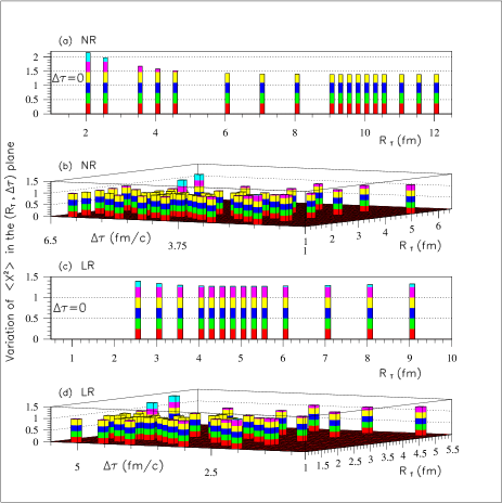
Figure 15: Zone in the ($R_{T},\Delta\tau$) plane investigated, leading to the determination of the most probable region where the minimum $\langle\chi^{2}\rangle$, associated to ($R_{T},\Delta\tau$), could be located. Parts (a) and (b) correspond to cases where the contribution of $K^{\star}$ were ignored. Parts (c) and (d) were estimated including their contribution to the kaon yield. In parts (a) and (c) we fixed $\Delta\tau=0$, and optimized only $R_{T}$. Figure extracted from Ref.padrol .

It was expected to be harder to differentiate both scenarios due to the lack of contribution from long-lived resonances. It was found that they could still be separated, with data favoring the non-resonance scenario at the 14.6 $Si+Au$ collisions (BNL/AGS). As in the two- pion interferometric analysis, the variation of the average $<\chi^{2}>$ per degrees of freedom in the ($q_{T},q_{L}$) plane was the significant quantity to look at, as can be seen n Fig. 16. The main fit results found in this analysis are summarized in Table 2. For more details, see Ref.padrol .

Figure 16: The number of standard deviations from unity of the average $<\chi^{2}>$ per degree of freedom is shown for increasing number of bins. In part (a), the transverse radius parameter, $R_{T}$, and the freeze-out spread, $\Delta\tau$, used for generating the theoretical plots, were optimized. In (b), only $R_{T}$ was optimized, whereas $\Delta\tau$ was fixed to be zero. Figure extracted from Ref.padrol .

The tests also ruled out the possibility of a zero decoupling proper-time conjectured by that experimental results of AGS/E859 Collaboratione859 . This can be seen from part (b) of Fig. 16: by fixing $\Delta\tau$ to be zero the numerical deviations of the average $<\chi^{2}>$ per degrees of freedom are completely meaningless.

II.6 II.4  SONOLUMINESCENCE BUBBLE

In the beginning of this review, we saw that the HBT interferometry was originally proposed for measuring the large sizes (of order $R\sim 10^{10}$ m) of stelar sources in radio-astronomy . On the other hand, in the totality of the cases discussed here so far, the dimensions went down to the order of the hadronic or to the nuclear size (roughly, $R\sim 10^{-15}$ m).

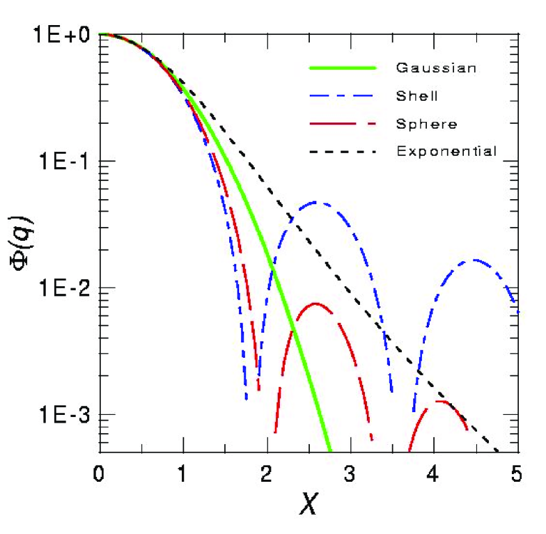
Figure 17: The upper part of the figure shows correlation functions plotted as function of $\Delta\omega=\omega_{1}-\omega_{2}=c(k_{1}-k_{2})$. Cases A to E correspond, respectively, to the first up to the fifth examples in Table 2. The lower part, shows the geometrical form factor $\Phi(q)$ plotted as a function of $X=\sqrt{-(1/2)[d^{2}\Phi(0)/dq^{2}]}q$. Figures extracted from Ref.hkp .

In between these two very different scales, Yogiro Hama, Takashi Kodama, and myself hkp discussed in 1995 an interesting approach to a beautiful problem, in a distinct environment. The focus was in a small sonoluminescent bubble, whose radius would lie in the range $R\sim 10^{-5}$m. The phenomenon had been discovered long time ago, in 1934, at the Univ. of Cologne, but its single bubble version was found out by Gaitan et al.sono1 only in 1988. In this last case, a single bubble of gas (usually filled with air) formed in water, is trapped by standing acoustic waves, contracting every 10-12 pico-sec approximately, and simultaneously emitting light. In other words, the sonoluminescence process converts the acoustic energy in a fluid medium into a short light pulse emitted from the interior of a collapsing small cavitating bubblesono1 . The spectrum of emitted light is very wide, extending from the visible to the ultraviolet regions. An important fact is that the light emission takes place within a very short period of time. The small size of the emission region and the short time scale of the emission process make it difficult to obtain precise geometrical and dynamical information about the collapsing bubble. Besides, a particular aspect of the emission process is still controversial: some authors attribute the light emission to the quantum-electrodynamic vacuum property based on the dynamical Casimir effectcasimir , whereas others consider that thermal processesthermal , such as a black-body type of radiation, should be the natural explanation. In Ref.hkp , we suggested that two-photon interferometry could shed some light to the problems raised above, by estimating the very small size and life-time of the single bubble sonoluminescence phenomenon. In fact, the simple existence of a HBT type of signal from such a collapsing bubble selects the scenario of explanation between the two classes mentioned above. This is possible because the emission processes are opposite in the case of thermal models and in the Casimir based ones. In the first case, the emission is chaotic, a condition that is essential for observing the two-identical particle HBT correlations, and an interferometric pattern would be observable. For the Casimir type of models, however, the emission is coherent and no HBT effect would be observable since, in that case, the correlation function acquires the trivial value $C(k_{1},k_{2})=1$ for all values of $k_{i}$.

In this work we neglect all the dynamical effects discussed in the previous studies, and considered that the space and time dependence would be decoupled as well. We adopted the notation used in Heinz2 , applied for our case.

$$C(\vec{k}_{1},\vec{k}_{2})=1+\frac{1}{2}\frac{|\tilde{S}(\vec{q},\vec{K})|^{2}}{\tilde{S}(0,\vec{k}_{1})\,\tilde{S}(0,\vec{k}_{2})}\,\;\;,$$ (57)

where

$$\tilde{S}(\vec{q},\vec{K})=\int d^{4}x\,e^{-iqx}\rho(x)\,j^{*}(\vec{k}_{1})j(\vec{k}_{2})\;,$$

$\vec{q}=\vec{k}_{1}-\vec{k}_{2}$ , $\vec{K}=(\vec{k}_{1}+\vec{k}_{2})/2\,$, and $j(\vec{k}_{i})$ is the amplitude for the emission of a photon with the wave-vector $\vec{k}_{i}$ at the source point $x$. The factor 1/2 in the second term of Eq. (57) comes from the spin 1 character of the photonHeinz2 .

We suggested a set of candidate models that could try and describe the system, as summarized in Table 3.

TABLE 3
Analytic expressions for some source parameterizations and the corresponding correlation functions are shown.

             Source $$\rho(r,t)$$

A:

B:

C:

D:

E:

As far as I know, no HBT experiment has been made yet with the photons emitted by the sonoluminescence bubble. T. Kodama and members of his group had initiated the experiment to produce single cavitating bubbles, with intension to perform the interferometric test I have just described above. In any case, the simple observation of a two-photon HBT correlation would be enough to rule out one of the two classes of models that aim at explaining the phenomenon, i.e., the ones based on the Casimir effect, in which the emission is coherent. It would automatically enforce the other class of thermal models, for which the emission is chaotic.

II.7 II.5  CONTINUOUS EMISSION

In Section II.2.1, we discussed the Bjorken Inside-Outside Cascade (IOC)Bj picture. It considers that, after high energy collisions, the system formed at the initial time $\tau=\tau_{0}$, thermalizes with an initial temperature $T_{0}$, evolving afterwards according to the ideal 1-D hydrodynamics, essentially the same as Landau’s version discussed in Section II.1, but with different initial conditions. During the expansion, the system gradually cools down and later decouples, when the temperature reaches a certain freeze-out value, $T_{f}$. In this model there is a simple relation between the temperature and the proper-time, i.e., $\tau\propto\tau_{0}\left(\frac{T_{0}}{T_{f}}\right)^{3}.$

A very interesting alternative picture of the particle emission was proposed by Grassi, Hama and Kodamaghk : instead of emitting particles only when these crossed the freeze-out surface, they considered that the process could occur continuously during the whole history of the expanding volume, at different temperatures. In this model, due to the finite size and lifetime of the thermalized matter, at any space-time point $x^{\mu}$ of the system, each particle would have a certain probability of not colliding anymore. So, the distribution function $f(x,p)$ of the expanding system would have two components, one representing the portion already free and another corresponding to the part still interacting, i.e., $f(x,p)=f_{free}(x,p)+f_{int}(x,p).$

In the Continuous Emission (CE) model, the portion of free particles is considered to be a fraction of the total distribution function, i.e., $f_{free}(x,p)={\cal P}f(x,p)\Longrightarrow f_{int}(x,p)=(1-{\cal P})f(x,p)$ or, equivalently,

$$f_{free}(x,p)=\frac{{\cal P}}{1-{\cal P}}f_{int}(x,p)\;\;.$$ (58)

The interacting part is assumed to be well represented by a thermal distribution function

$$f_{int}(x,p)\approx f_{th}(x,p)=\frac{g}{(2\pi)^{3}}\frac{1}{\exp{\ \left[p.u(x)/T(x)\right]}\pm 1}\;\;,$$ (59)

which poses a constraint on the applicability of the picture, since by continuously emitting particles the system would be too dilute to be considered in thermal equilibrium in its late stages of evolution. In Eq. (59), $u^{\mu}$ is the fluid velocity at $x^{\mu}$ and $T$ is its temperature in that point.

The fraction of free particles ${\cal P}$ at each space-time point, $x^{\mu}$, was computed by using the Glauber formula, i.e., ${\cal P}=\exp{\ \left(-\int_{t}^{t_{out}}n(x^{\prime})\sigma v_{rel}dt^{\prime}\right)},$where $t_{out}=t+(-\rho\cos\phi+\sqrt{R_{T}^{2}-\rho^{2}\sin^{2}\phi})/(v\sin\theta).$

The model also considered that, initially, the energy density could be approximated by a constant (i.e., $\epsilon=\frac{\pi^{2}}{10}T_{0}^{4}$ for all the points with $\rho\leq R_{T}$ and zero for $\rho>R_{T}$). Then, the probability ${\cal P}$ may be calculated analytically, resulting in ${\cal P}=(\tau/\tau_{out})^{a};\;\;a\sim 3\frac{1.202}{\pi^{2}}T_{0}^{3}\tau_{0}\sigma v_{rel},$where $v_{rel}\approx 1$. The factor ${\cal P}$ can be interpreted as the fraction of free particles with momentum $p^{\mu}$ or, alternatively, as the probability that a particle with momentum $p^{\mu}$ escapes from $x^{\mu}$ without further collisions.

Their early results for the spectra can be seen in Ref.ghk and in the review by Frederique Grassi, in this volume, which is a good source of further details and discussions on the Continuous Emission model.

Later, in collaboration with F. Grassi, Y. Hama, and O. Socolowskipghs , we developed the formulation for applying this new freeze-out criterium into $\pi\pi$ interferometry. Naturally, we would like to further explore if the above model would present striking differences when compared to the standard freeze-out picture (FO). One expectation would be that the space-time region from which the particles were emitted would be quite different in both scenarios. In particular, as we saw in Section II.1 and II.2.2, a non-instantaneous emission process strongly influences the behavior of the correlation function. Being so, a sizable difference was expected when comparing the instant freeze-out hypothesis and the continuous emission version, since in this last one, the emission process is expected to take much longer.

For treating the identical particle correlation within the continuous emission picture, instead of using the Covariant Current Ensemble formalism discussed in item II.2, we adopted a different but equivalent form for expressing the amplitudes in Eq. (26) as in Ref.ghk . Then, the single-inclusive distribution, can be written as

$$G(k_{i},k_{i})=\int d^{4}x\;{\cal D}_{\mu}\left[k_{i}^{\mu}f_{free}\right]\;\;,$$ (60)

where ${\cal D}_{\mu}$ is the generalized divergence operator. In Ref.ghk , it was shown that, in the limit of the usual freeze-out, Eq. (60) is reduced to the Cooper-Frye integral, $E\frac{d^{3}N}{dp^{3}}=\int_{T_{f}}d\sigma_{\mu}p^{\mu}f(x,p)$, over the freeze-out hyper-surface $T=T_{f}$, being $d\sigma_{\mu}$ the vector normal to this surface. Or equivalently, Eq. (60 ) in the instant freeze-out picture is reduced to Eq. (28), with the currents given by Eq. (29), or even by Eq. (30), which is a simplified parametric form of describing thermal currents used for obtaining analytical results in the Bjorken picture. We see more easily that it is indeed the limit if we replace the distribution function in Eq.(59) by its Boltzmann limit. We see more clearly that Eq. (28), or Eq. (38) in the Bjorken picture, are the natural limits of the proposed continuous emission spectrum, in case of instant freeze-out.

Analogously, the two-particle complex amplitude is written as

$$G(k_{1},k_{2})=\int d^{4}xe^{iqx}\;\{{\cal D}_{\mu}\left[k_{1}^{\mu}f_{free}\right]\}^{\frac{1}{2}}\;\{{\cal D}_{\mu}\left[k_{2}^{\mu}f_{free}\right]\}^{\frac{1}{2}}\;\;.$$ (61)

We saw above that the expression for the spectrum is reduced to the one in the Covariant Current Ensemble formalism in the limit of the instant freeze-out. Analogously, the above expression in this limit should yield to the result in Eq. (27). We see that this is indeed the case if we replace the individual momenta $k_{i}^{\mu}$ in E.(61) by the average momentum of the pair, $K^{\mu}=\frac{1}{2}(k_{1}^{\mu}+k_{2}^{\mu})$. This replacement is even more natural, if we remember that the $K^{\mu}$ is the momentum appearing in the Wigner formulation of interferomtrypratt ; pgg ; gb ; heinz1 ; hpb . And, it was shown in Ref. pgg that this also is reduced to the Covariant Current Ensemble for minimum packets and having the packet width equated to the pseudo-thermal temperature, as discussed in Section II.2.2. When this is assumed, also a substantial simplification is obtained in Eq.(61), which could then be written as

$$G(q,K)=\int d^{4}x\;e^{iq^{\nu}x_{\nu}}\;{\cal D}_{\mu}\left[K^{\mu}f_{free}\right]\;\;.$$ (62)

We compare next the results for these two very different scenarios by means of the two-pion correlation functions, assuming the Bjorken picture for the system, i.e., neglecting the transverse expansion. For the instant FO case, we use Eq.(36) and (38) for obtaining $C(q,K)$. For the CE case, we use Eq.(60) and (62) , writing the four-divergence and the integrals in cylindrical coordinates, using the symmetry of the problem, which leads to a simpler expression:

$$\!\!\!\!G(q,K)=$$

$$\!\!\!\!\!\!\frac{1}{(2\pi)^{3}}\int_{0}^{2\pi}d\phi\int_{-\infty}^{+\infty}d\eta\;\{\int_{0}^{R_{T}}\rho\,d\rho\;\tau_{{\cal F}}\,M_{T}\,\cosh(Y-\eta)$$

$$\!\!\!\!\!\!\times e^{i[\tau_{{\cal F}}(q_{0}\cos\eta-q_{L}\sinh\eta)-\rho q_{T}\cos(\phi-\phi_{q})]}\;$$

$$\!\!\!\!\!\!+\int_{\tau_{0}}^{+\infty}\!\!\tau d\tau\rho_{{\cal F}}K_{T}\cos\phi\,e^{i[\tau(q_{0}\cos\eta-q_{L}\sinh\eta)-\rho_{{\cal F}}q_{T}\cos(\phi-\phi_{q})]}\}$$

$$\!\!\!\!\!\!\times\;\frac{e^{-M_{T}\cosh(Y-\eta)/T_{ps}(x)}}{(1-{\bf{\cal P}}_{{\cal F}})}\;,$$ (63)

where $M_{T}=\sqrt{K_{T}^{2}+M^{2}};\;M^{2}=K^{\mu}K_{\mu}-\frac{1}{4}q^{\mu}q_{\mu};\;K^{\mu}=\frac{1}{2}(k_{1}^{\mu}+k_{2}^{\mu})$; $Y$ is the rapidity corresponding to $\vec{K}$, $\phi$ is the azimuthal angle with respect to the direction of $\vec{K}$, $\phi_{q}$ is the angle between the directions of $\vec{q}$ and $\vec{K}$, and

$$\tau_{{\cal F}}=\frac{-\rho\cos\phi+\sqrt{R_{T}^{2}-\rho^{2}\sin^{2}\phi}}{(k_{T}/E)[\sqrt{\sinh^{2}\eta+{\bf{\cal P}}_{{\cal F}}^{-2/a}}-\cosh\eta]}\;\;.$$

$$\rho_{{\cal F}} = -\tau\;(k_{T}/E)\cos\phi[\sqrt{\sinh^{2}\eta+{\bf{\cal P}}_{{\cal F}}^{-2/a}}-\cosh\eta]\;\pm\;$$

$$\sqrt{R_{T}^{2}-\tau^{2}(\frac{k_{T}}{E})^{2}\sin^{2}\phi\;[\sqrt{\sinh^{2}\eta+{\bf{\cal P}}_{{\cal F}}^{-2/a}}-\cosh\eta]^{2}}.$$

The spectrum is obtained from the expression (63), by replacing $K^{\mu}\rightarrow k_{i}^{\mu}$, $M\rightarrow m$, and $q^{\mu}\rightarrow 0$. In Eq. (63), $\tau_{{\cal F}}$ and $\rho_{{\cal F}}$, whose expressions are written above, are the limiting values corresponding to the escape probability ${\cal P}_{{\cal F}}$, which we fix to be ${\cal P}_{{\cal F}}\approx 0.5$, approximate value chosen for the sake of simplicity and for guaranteeing that the thermal assumption still holds in systems with finite size and finite lifetime. The rest of the emission for ${\cal P}_{{\cal F}}>0.5$ is assumed to be instantaneous, as in Eq. (36) and (38).

The complexity of the expressions for the Continuous Emission (CE) case suggested that we should look into special kinematical zones for investigating the differences between this scenario and the instant freeze-out picture. For details and discussions, see Ref.pghs . I summarize some of them. First, we observed that the correlation function $C(q_{O},q_{L})$ plotted versus the outward momentum difference, ${\bf q_{O}}$, exhibited the well-know dependence on the average momentum of the pair, $K_{T}$, discussed earlier in this section, in both cases. However, it was enhanced in the CE scenario, as expected, since the emission duration is longer in this case than in the standard freeze-out picture. We also observed a slight variation with $K_{T}$ of the correlation function versus ${\bf q_{S}}$ in the CE, differently from the instant freeze-out case, were it was absent, since we were considering only the longitudinal expansion of the system and no transverse flow. This result showed the tendency of the curve versus ${\bf q_{S}}$ to become slightly narrower for increasing $K_{T}$, an opposite tendency as compared to the curves plotted as functions of ${\bf q_{O}}$.

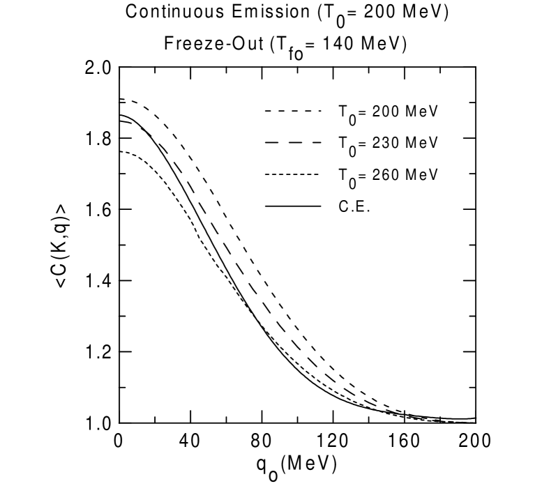
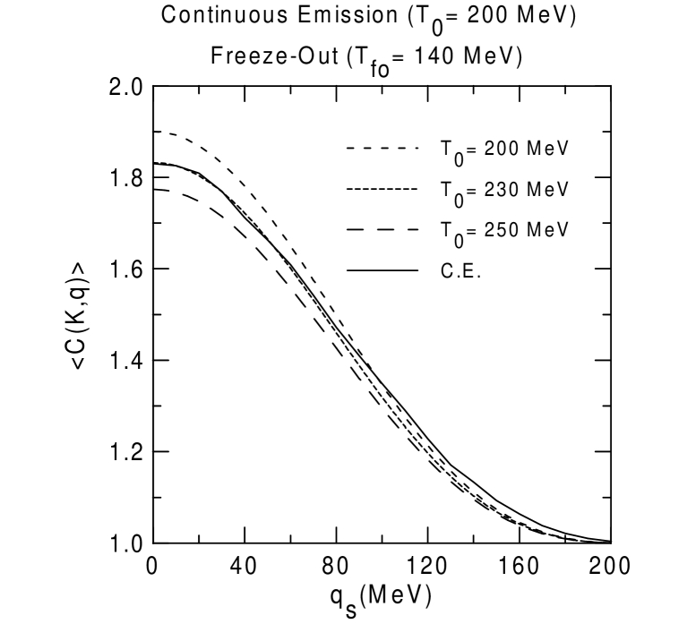
Figure 18: The average correlation function $\langle C\rangle_{\pi\pi}$ is shown versus $q_{L}$, $q_{O}$, and $q_{S}$, averaging over, respectively, ($q_{S}$ , $q_{O}$), ($q_{L}$ , $q_{S}$), and ($q_{L}$ , $q_{O}$). Comparison is made of the (solid) curve for the CE scenario with three others corresponding to the usual freeze-out at $T_{fo}=140$ MeV, but with different initial temperatures, whose values are shown in the plot. Plots extracted from Ref.pghs .

We also studied more realistic situations, where the correlation function was averaged over kinematical zones. Using the azimuthal symmetry of the problem, we defined the transverse component $K_{T}$ along the x-axis, such that $\vec{K}=(K_{T},0,K_{L})$. We then averaged over different kinematical regions, mimicking the experimental cuts, by integrating over the components of $\vec{q}$ and $\vec{K}$ (except over the plotting component of $\vec{q}$). For illustration, we considered the kinematical range of the CERN/NA35na35b experiment on S+A collisions at 200 AGeV, as

$$\!\!\!\langle C(q_{L})\rangle=1+$$

$$\!\!\!\!\!\!\!\!\!\frac{\int^{180}_{-180}dK_{L}\int^{600}_{50}dK_{T}\int^{30}_{0}dq_{S}\int^{30}_{0}dq_{o}C(K,q)|G(K,q)|^{2}}{\int^{180}_{-180}dK_{L}\int^{600}_{50}dK_{T}\int^{30}_{0}dq_{S}\int^{30}_{0}dq_{o}C(K,q)G(k_{1},k_{1})G(k_{2},k_{2})}.$$

With the previous equation we estimated the average theoretical correlation functions versus $q_{L}$, $q_{O}$ and $q_{S}$, comparing the results for CE and for FO scenarios. First, we considered the case in which the initial temperature was the same in both cases ($T_{0}=200$ MeV) and compared the CE prediction with two outcome curves corresponding to two FO temperatures, $T_{fo}=140$ and $T_{fo}=170$MeV. We observed that the same initial temperature led to entirely different results in each case. The details are shown and discussed in Ref. pghs . In the second situation, we relaxed the initial temperature constraint and studied the similarity of the curve in the CE scenario corresponding to a certain value of $T_{0}$, and compared to three different curves in the FO scenario, for which the freeze-out temperature was fixed $T_{fo}=140$ MeV. Each one of these curves in the standard FO case corresponded to a different initial temperature. The purpose here was to investigate, as usually done when trying to describe the experimental data, which initial temperatures in the FO scenario would lead to the curve closest to the one generated under the CE hypothesis. The results are shown in Fig. 18. Usually the shape of the correlation curve is very different in both cases, the one corresponding to the CE being highly non-Gaussian, mainly in the upper left plot of Fig. 18. In this particular one, we see that the CE correlation curve can be interpreted as showing the history of the hot expanding matter. For instance, the tail of $\langle C\rangle$ reflects essentially the early times, when the size of the system is small and the temperature is high, since the tail of the CE curve is closer to the FO one corresponding to the highest initial temperature. On the contrary, the peak region corresponds to the later times where the dimensions of the system are large and the temperature low (see the compatibility with the FO curve corresponding to the lowest initial temperature).

II.8 II.6  FINITE SIZE EFFECTS

II.9 II.6.1  PION SYSTEM

In 1998, a pos-doctoral fellow from China, Qing-Hui Zhang, joined the group, spending one year with us. Together, we investigated the effects of finite source sizes (boundary effects) on $\pi^{\pm}\pi^{\pm}$ interferometry. We derived a general formulation for spectrum and two-particle correlation, adopting a density matrix suitable for treating the charged pion cases in the non-relativistic limitzp .

A few hypotheses inspired that study. First, we considered pions, the most abundant particles produced in relativistic heavy-ion collisions, to be quasi-bound in the system, with the surface tensionshu ; MW95 ; SRSAS97 acting as a reflecting boundary. In this regard, the pion wave function could be assumed as vanishing outside this boundary. As usual, we also considered that these particles become free when their average separation is larger than their interaction range and we assumed this transition to happen very rapidly, in such a way that the momentum distribution of the pions would be governed by their momentum distribution just before they freeze out. We then studied the modifications on the observed pion momentum distribution caused by the presence of this boundary. We also investigated its effects on the correlation function, which is known to be sensitive to the geometrical size of the emission region as well as to the underlying dynamics. In this formalism, the single-pion distribution can then be written as

$$P_{1}({\bf p}) = \langle\hat{\psi}^{\dagger}({\bf p})\hat{\psi}({\bf p})\rangle=\sum_{\lambda}\sum_{\lambda^{\prime}}\tilde{\psi}_{\lambda}^{*}{(\bf p)}\tilde{\psi}_{\lambda^{\prime}}^{*}{(\bf p)}\langle\hat{a}^{\dagger}_{\lambda}\hat{a}_{\lambda^{\prime}}\rangle$$ (64)

$$= \sum_{\lambda}N_{\lambda}\tilde{\psi}^{*}_{\lambda}({\bf p})\tilde{\psi}_{\lambda}({\bf p})\;\;,$$

where the last equality follows from the fact that the expectation value $\langle\hat{a}^{\dagger}_{\lambda}\hat{a}_{\lambda^{\prime}}\rangle$ is related to the occupation probability of the single-particle state $\lambda$, $N_{\lambda}$, by $\langle\hat{a}^{\dagger}_{\lambda}\hat{a}_{\lambda^{\prime}}\rangle=\delta_{\lambda,\lambda^{\prime}}N_{\lambda}\;;\;$$a_{\lambda}$ ($a^{\dagger}_{\lambda}$) is the annihilation (creation) operator for destroying (creating) a pion in a quantum state characterized by a quantum number $\lambda$. In Eq. (64) $\hat{\psi}^{(\dagger)}({\bf p})=\sum_{l}\hat{a}^{(\dagger)}_{l}\tilde{\psi}^{(*)}_{l}({\bf p})$, where $\hat{a}^{\dagger}$ ($\hat{a}$) is the pion creation (annihilation) operator, and $\tilde{\psi}_{l}$ is one of the eigenfunctions belonging to a localized complete set, satisfying orthogonality and completeness relations.

For a bosonic system in equilibrium at a temperature $T$ and chemical potential $\mu$, $N_{\lambda}$ it is represented by the Bose-Einstein distribution

$$N_{\lambda}=\frac{1}{\exp{\left[\frac{1}{T}(E_{\lambda}-\mu)\right]}-1}\;\;.$$ (65)

The above formula coincides with the one employed in Ref.MW95 for expressing the single-pion distribution.

The normalized expectation value of an observable $A$ is given by

$$\langle\hat{A}\rangle=\frac{tr\{\hat{\rho}\hat{A}\}}{tr\{\hat{\rho}\}}\;\;;\;\;\hat{\rho}=\exp\left[-\frac{1}{T}(\hat{H}-\mu\hat{N})\right]=\prod_{l}\hat{\rho}{{}_{l}}\;,\;$$ (66)

where $\hat{\rho}$ is the density matrix operator for the bosonic system, and $\hat{\rho}_{l}=\exp\left[-\frac{1}{T}(\hat{H}_{l}-\mu\hat{N}_{l})\right],\;$with

$$\hat{H}=\sum_{l}\hat{H}_{l};\;\;\;\;\hat{H}_{l}=E_{l}\hat{N}_{l};\;\;\;\;\hat{N}=\sum_{l}\hat{N}_{l}\;,$$ (67)

respectively, the Hamiltonian and number operators; $\mu$ is the chemical potential, fixed to be zero in the results we present here.

Similarly, the two-pion distribution function can be written as

$$\!\!\!\!\!\!\!\!\!P_{2}({\bf p_{1},p_{2}})=\!\!\!\!\!\!\!\!\!\sum_{\lambda_{1},\lambda_{2},\lambda_{3},\lambda_{4}}\tilde{\psi}_{\lambda_{1}}^{*}({\bf p_{1}})\tilde{\psi}_{\lambda_{2}}^{*}({\bf p_{2}})\tilde{\psi}_{\lambda_{3}}({\bf p_{1}})\tilde{\phi}_{\lambda_{4}}({\bf p_{2}})$$ (68)

$$\;\;\;\;\;\;\;\;\;\;\;\;\;\;\;\;\;\;\;\;\;\;\;\;\langle\hat{a}^{\dagger}_{\lambda_{1}}\hat{a}^{\dagger}_{\lambda_{2}}\hat{a}_{\lambda_{3}}\hat{a}_{\lambda_{4}}\rangle$$

$$= \sum_{\lambda_{1},\lambda_{2},\lambda_{3},\lambda_{4}}\tilde{\psi}_{\lambda_{1}}^{*}({\bf p_{1}})\tilde{\psi}_{\lambda_{2}}^{*}({\bf p_{2}})\tilde{\psi}_{\lambda_{3}}({\bf p_{1}})\tilde{\phi}_{\lambda_{4}}({\bf p_{2}})$$

$$\left[\langle\hat{a}^{\dagger}_{\lambda_{1}}\hat{a}_{\lambda_{3}}\rangle\langle\hat{a}^{\dagger}_{\lambda_{2}}\hat{a}_{\lambda_{4}}\rangle_{\lambda_{1}\neq\lambda_{2}}\right.+\langle\hat{a}^{\dagger}_{\lambda_{1}}\hat{a}_{\lambda_{4}}\rangle\langle\hat{a}^{\dagger}_{\lambda_{2}}\hat{a}_{\lambda_{3}}\rangle_{{}_{\lambda_{1}\neq\lambda_{2}}}$$

$$\left.+\langle\hat{a}^{\dagger}_{\lambda_{1}}\hat{a}^{\dagger}_{\lambda_{2}}\hat{a}_{\lambda_{3}}\hat{a}_{\lambda_{4}}\rangle_{\lambda_{1}=\lambda_{2}=\lambda_{3}=\lambda_{4}}\right]$$

$$= P_{1}({\bf p_{1}})P_{1}({\bf p_{2}})+|\sum_{\lambda}N_{\lambda}\tilde{\psi}_{\lambda}^{*}({\bf p_{1}})\tilde{\psi}_{\lambda}({\bf p_{2}})|^{2}.$$

Since we are considering the case of two indistinguishable, identically charged pions, then $\langle\hat{a}_{\lambda}^{\dagger}\hat{a}_{\lambda}^{\dagger}\hat{a}_{\lambda}\hat{a}_{\lambda}\rangle=2\langle\hat{a}^{\dagger}_{\lambda}\hat{a}_{\lambda}\rangle^{2}.$  From the particular form proposed for the density matrix it follows that $\langle\hat{a}^{\dagger}_{\lambda}\hat{a}^{\dagger}_{\lambda}\rangle=\langle\hat{a}_{\lambda}\hat{a}_{\lambda}\rangle=0$, showing that it would not be suited for describing $\pi^{0}\pi^{0}$ and $\pi^{+}\pi^{-}$ cases. For this purpose, the formalism proposed in Ref.YS94 is more adequate.

The two-particle correlation can be written as

$$C_{2}({\bf p_{1},p_{2}}) = \frac{P_{2}({\bf p_{1},p_{2}})}{P_{1}({\bf p_{1}})P_{1}({\bf p_{2}})}$$

$$= 1+\frac{|\sum_{\lambda}N_{\lambda}\psi_{\lambda}^{*}({\bf p_{1}})\psi_{\lambda}({\bf p_{2}})|^{2}}{\sum_{\lambda}N_{\lambda}|\psi_{\lambda}({\bf p_{1}})|^{2}\sum_{\lambda}N_{\lambda}|\psi_{\lambda}({\bf p_{2}})|^{2}}\;\;.$$

In Ref. zp we illustrated the formalism by means of two examples. The first considered that the produced pions were bounded inside a confining sphere with radius $R$. In the second, they were inside a cubic box with size $L$. Since the results were similar in both cases, I will briefly discuss here only the first one. We estimated Eq.(64) for the confining sphere of radius $R$ for studying the boundary effects on the spectrum. The results can be summarized by looking directly into the top left plot in Fig. 19, where we also show the curve corresponding to the limit of very large system ($R\rightarrow\infty$). We see that the finite size affects the spectrum by depleting the curve at small values of the pion momentum and, at the same time, rising and broadening the curve at large $p$ (momentum conservation).

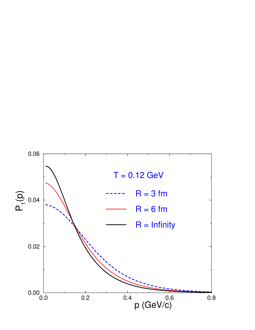
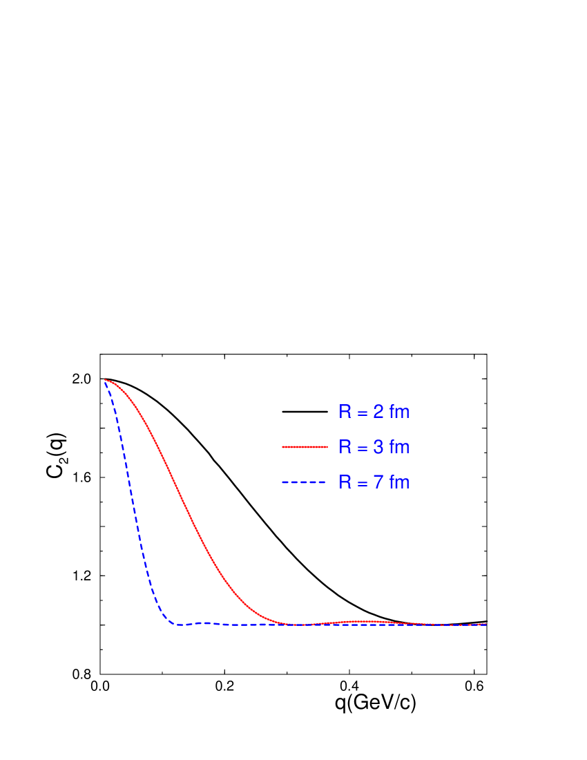
Figure 19: The top plot shows the spectrum in the example of pions confined in the sphere of radius $R$. The top right plot shows $C_{\pi\pi}(q)$ versus $q$, for three different values of the source radius. The plot in the bottom shows that the correlation function shrinks for increasing average momentum, $K$, in opposition to the behavior seen in Fig. 7 and for expanding systems, in general. Plots extracted from Ref.zp .

For studying the behavior of the correlation function we estimated Eq. (LABEL:pi2) in the case of the bounding sphere. Some results are shown in the top right plot of Fig. 19 and they are as expected: the correlation shrinks (i.e., the probed source dimension increases) with increasing values of the radius. Nevertheless, the bottom curve, corresponding to $C(q,K)$ versus $q$, shows an unexpected behavior for different values of the average momentum $K$. Contrary to what is observed in expanding system, the correlation function becomes narrower (probed region enlarges) with increasing $K$. However, the example shown for illustration does not take into account the expansion of the system. The variation with $K$ merely reflects the strong sensitivity of the results to the dynamical matrix adopted in the formulation. It is related to the weight factor $N_{\lambda}$, in Eq. (LABEL:pi2): pions with larger momenta come from higher quantum states $\lambda$, which correspond to a smaller spread in coordinate space. But, due to the Bose-Einstein form of the weight factor, large quantum states give a small contribution to the source distribution, causing the effective source radius to appear larger. To emphasize this we include in the bottom plot the narrowest curve, corresponding to fixing $N_{\lambda}=1$ (or equivalently, by considering $T\gg 1$ in the Bose-Einstein distribution, which makes $C(q,K)$ insensitive to $K$, due to the large temperature). This limit allows for an analytical expression,

$$C_{2}(q)=1+\frac{9}{q^{4}R^{6}}\left[R\cos(qR)-\frac{\sin(qR)}{q}\right]^{2},\;$$ (70)

which is shown in the lowest curve of the bottom plot of Fig. 19. Underneath this curve, shown by little circles in the same plot, is the numerically generated curve for $N_{\lambda}=1$, confirming the correcteness of our result.

II.10 II.6.2  $Q$-BOSON SYSTEM

More recently, Qing-Hui Zhang and I extended the above formalism for treating the interferometry of two $Q$-bosons. The concept of quons was suggestedgreenberg as an artifact for reducing the complexity of interacting systems, at the expense of deforming their commutation relations by means of a deformation parameter, $Q$. Then, this could be seen as an effective parameter, encapsulating the essential features of complex dynamics.

We derived a formalism suitable for describing spectra and two-particle correlation function of charged $Q$-bosons, which we considered as bounded in a finite volume. We adopted the $Q$-boson type suggested by Anchishkin et al.AGI , according to which the $Q$-bosons are defined by the following algebra of creation ($\hat{a}^{\dagger}$) and annihilation operators ($\hat{a}$): $\hat{a}_{l}\hat{a}_{l^{\prime}}^{\dagger}-Q^{\delta_{l,l^{\prime}}}\hat{a}_{l^{\prime}}^{\dagger}\hat{a}_{l}=\delta_{l,l^{\prime}},\;[\hat{a}_{l},\hat{a}_{l^{\prime}}]=[\hat{a}_{l}^{\dagger},\hat{a}_{l^{\prime}}^{\dagger}]=0,\;[\hat{N}_{l},\hat{a}_{l^{\prime}}]=-\delta_{l,l^{\prime}}\hat{a}_{l}\;[\hat{N}_{l},\hat{a}_{l^{\prime}}^{\dagger}]=\delta_{l,l^{\prime}}\hat{a}_{l}^{\dagger},\;[\hat{N}_{l},\hat{N}_{l^{\prime}}]=0;$ $\hat{N}_{l}$ is the number operator, $\hat{N}_{l}=\sum_{s=1}^{\infty}\frac{(1-Q)^{s}}{(1-Q^{s})}(\hat{a}_{l}^{\dagger})^{s}(\hat{a}_{l})^{s}.$ In the limit $Q=1$, the regular bosonic commutation relations are recovered. The deformation parameter $Q$ is a C-number, here assumed to be within the interval $[0,1]$.

The single-inclusive, $P_{1}({\bf p})$, and the two-particle distributions are derived in a similar way as in the case of regular pions discussed above. In the $Q$-boson case, Eq.(64) continues to hold, but the weight factor, $N_{\lambda}$, related to the occupation probability of a single-particle state $l$, no longer is as written in Eq.(65), but is changed into a modified Bose-Einstein distribution,

$$N_{l}=\frac{1}{\exp{\left[\frac{1}{T}(E_{l}-\mu)\right]}-Q}\;.$$ (71)

The two-particle correlation function as also modified, and is written as

$$C_{2}({\bf p_{1},p_{2}})=\frac{P_{2}({\bf p_{1},p_{2}})}{P_{1}({\bf p_{1}})P_{1}({\bf p_{2}})}=$$

$$=1+\left\{\sum_{l}N_{l}|\tilde{\psi}_{l}({\bf p_{1}})|^{2}\sum_{l}N_{l}|\tilde{\psi}_{l}({\bf p_{2}})|^{2}\right\}^{-1}\times$$

$$\;\;\;\sum_{l,l^{\prime}}\;\ N_{l}N_{l^{\prime}}\tilde{\psi}_{l}^{*}({\bf p_{1}})\tilde{\psi}_{l^{\prime}}^{*}({\bf p_{2}})\tilde{\psi}_{l}({\bf p_{2}})\tilde{\psi}_{l^{\prime}}({\bf p_{1}})\times$$

$$\left\{1-\delta_{l,l^{\prime}}(1-Q)\cdot\frac{\exp(\frac{1}{T}(E_{l}-\mu))+Q}{\exp(\frac{1}{T}(E_{l}-\mu))-Q^{2}}\right\}\;\;.$$ (72)

We apply this formulation by means of similar models as in Ref.zp , for the confining sphere of radius $R$. We studied the effects of different values of $Q$ on the correlation function, under different values of the pair average momentum, $K_{T}$. In Fig. 20 we show the boundary effects on the $Q$-boson spectrum and on the two-$Q$-boson correlation function. We also included in that plot the behavior of the of the two-$Q$ boson intercept parameter, $\lambda$, defined by $\lambda=C({\bf q=0},{\bf K})-1$. The top two plots in Fig. 20 reproduce the basic characteristics seen in Fig. 19, in particular, the correlation function narrows as the average momentum, $K$, grows. There is, however, a new result: the maximum of the correlation function drops as the deformation parameter, $Q$, increases. This can also be seen by looking into the bottom plot of the intercept $\lambda$, as a function of $Q$.

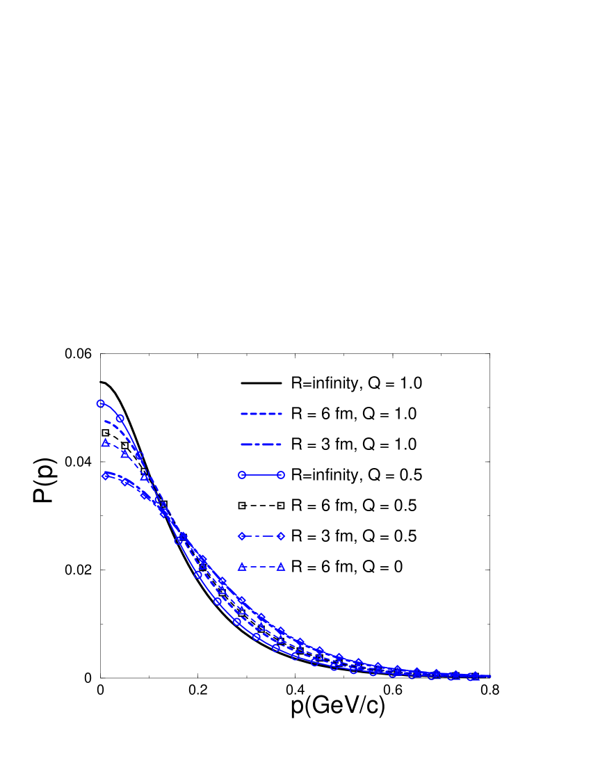
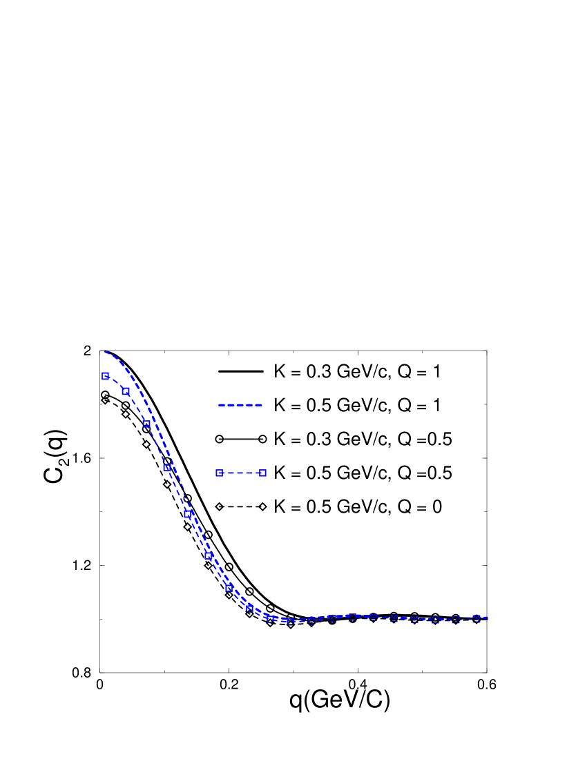
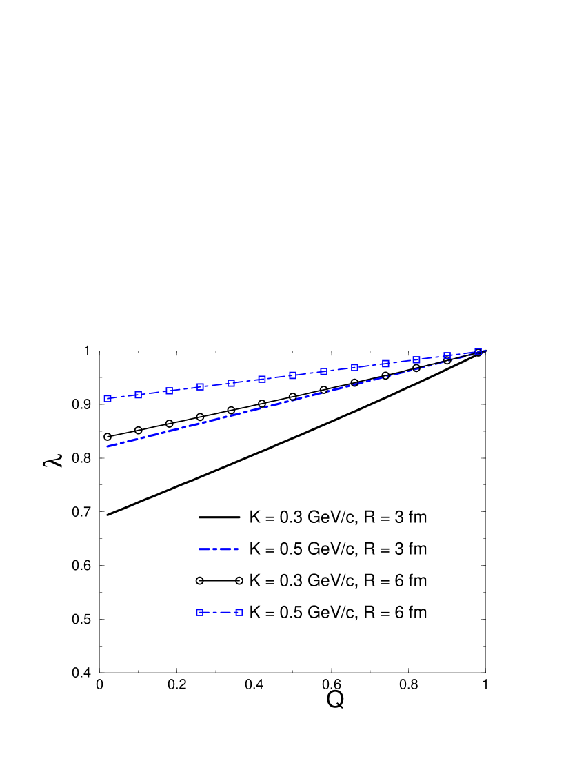
Figure 20: The results shown here were obtained by considering the $Q$-bosons confines inside a three-dimensional sphere of radius $R$. In the three plots above, the temperature was fixed to $T=0.12$ GeV and the chemical potential, $\mu=0$. The top left plot corresponds to the normalized spectrum (in arbitrary units) vs. momentum $|$p$|$ (in GeV/c). The solid lines correspond to the case $R\rightarrow\infty$, the dotted ones to $R=6$ fm, and the dashed lines correspond to the case, $R=3$ fm/c. The bare lines refer to $Q=1.0$ and the ones with symbols, to $Q=0.5$ ($Q=0$). The top right plot shows the two-pion correlation vs. momentum difference $|{\bf q}|$ (in GeV/c), for a $R=3$ fm sphere. The solid lines correspond to mean momentum $K=0.3$ GeV/c and the dashed ones, to the case $K=0.5$ GeV/c. The bare lines refer to the case of $Q=1.0$ and the ones with symbol, to $Q=0.5$ ($Q=0$). The bottom plot shows the intercept parameter, $\lambda$, vs. the deformation $Q$. The solid lines correspond to the mean momentum $K=0.3$ GeV/c and dashed ones to the case $K=0.5$ GeV/c. The bare lines refer to the case $R=3$ fm and the ones with symbols, to $R=6$ fm. Plots extracted from Ref.zp2 .

We also derived a generalized Wigner function for the $Q$-boson interferometry, which would reduce to the regular one in the limit of $Q\rightarrow 1$. For that, we define the Wigner function associated to the state $l$ as

$$g_{l}({\bf x},{\bf K})=\int\frac{d^{3}\Delta x}{(2\pi)^{3}}\;e^{-i{\bf K}.{\bf\Delta x}}\psi_{l}^{*}({\bf x}+\frac{\bf\Delta x}{2})\psi_{l}({\bf x}-\frac{\bf\Delta x}{2})\;.$$ (73)

We proceeded analogously to define the equivalent function for the integration in ${\bf y}$ and ${\bf\Delta y}$, remembering that $g_{l}({\bf x},{\bf K})=g_{l}^{*}({\bf x},{\bf K})$. Then, denoting by

$$g({\bf x},{\bf K})=\sum_{l}N_{l}\;g_{l},$$ (74)

we finally defined the generalized Wigner function of the problem as

$$g({\bf x},{\bf K};{\bf y},{\bf K})=g({\bf x},{\bf K})g({\bf y},{\bf K})\;-\;(1-Q)\times$$

$$\hskip-31.2982pt\sum_{l}\left\{N_{l}^{2}\left[\frac{\exp(\frac{1}{T}(E_{l}-\mu))+Q}{\exp(\frac{1}{T}(E_{l}-\mu))-Q^{2}}\right]g_{l}({\bf x},{\bf K})\;g_{l}({\bf y},{\bf K})\right\}.$$ (75)

We see that, for $Q=1$, the above expression is reduced to the usual result of the original Wigner function, i.e.,

$$g({\bf x},{\bf K};{\bf y},{\bf K})=g({\bf x},{\bf K})g({\bf y},{\bf K})\;.$$ (76)

On the other hand, for $Q=0$, Eq. (75) is identically zero for single modes only, as it would be expect in the limit of Boltzmann statistics. Nevertheless, in the multi-mode case, there seems to be some sort of residual correlation among $Q$-bosons even in the classical limit.

By means of this Wigner function, the two-$Q$-boson correlation function can be rewritten as

$$C_{2}({\bf p_{1},p_{2}})=1+\frac{\int\int e^{-i{\bf q}.({\bf x}-{\bf y})}g({\bf x},{\bf K};{\bf y},{\bf K})d{\bf x}d{\bf y}}{\int g({\bf x},{\bf p_{1}})d{\bf x}\int g({\bf y},{\bf p_{2}})d{\bf y}}$$ (77)

Particularly interesting is the approach in Ref.gastao , where it was shown that the composite nature of the particles (pseudo-scalar mesons) under study could result into deformed structures linked to the deformation parameter $Q$. In that reference this parameter is then interpreted as a measure of effects coming from the internal degrees of freedom of composite particles (mesons, in our case), being the value of $Q$ dependent on the degree of overlap of the extended structure of the particles in the medium. Being so, the $Q$-parameter could be related to the power of probing lenses, for mimicking the effects of internal constituents of the bosons. In this case, and for high enough magnification, the bosonic behavior of the $Q$-bosons could be blurred by the fermionic effect of their internal constituents, which would result in decreasing the value of $Q$. Our results on the two-$Q$-boson interferometry are compatible with this interpretation, as explained in detail in Ref.zp2 .

II.11 II.7  NON-EXTENSIVE STATISTICS AND HBT

Sérgio M. Antunessma , working under my supervision and in collaboration with G. Krein during his Master Degree, studied the effects of Tsallistsallis non-extensive statistics on the two-particle correlations and spectra. In this work, a very simple starting hypothesis was made: that under certain circumstances, the Boltzmann limit to the pion distribution could be replaced by an equivalent approximate expression derived within the non-extensive statistics. This concept of non-extensivity could be summarized very briefly by the relation: $S_{q_{T_{s}}}(A+B)=S_{q_{T_{s}}}(A)+S_{q_{T_{s}}}(B)+(1-q_{T_{s}})S_{q_{T_{s}}}(A)S_{q_{T_{s}}}(B)$, i.e., the entropy of a system formed by two independent sub-systems $A$ and $B$, no longer is the sum of the entropy of the two subsystems (note that by independent it is meant that the probability of the composite system factorizes as $p_{A+B}=p_{A}+p_{B}$). The parameter $q_{Ts}$ is a measure of the degree of non-extensivity of the system and the Boltzmann-Gibbs statistics is recovered in the limit $q_{T_{s}}\rightarrow 1$. From the definition of the generalized entropy in the Tsallistsallis formulation, it is possible to obtain approximate analytical expressions, for instance, for the mean occupation numberntsall

$$\hskip-34.14322pt\exp\{[-(E(p,r)-\mu]/T\}\longrightarrow$$

$$\{1+(q_{T_{s}}-1)[(E(p,r)-\mu]/T\}^{-1/(q_{T_{s}}-1)}\;,$$ (78)

which is reduced to the Boltzmann distribution for $q_{T_{s}}\!\!\!\rightarrow\!\!1$, where $T$ is the temperature and $\mu$, the chemical potential. The form given in Eq.(78) is, however, valid for $q_{Ts}$ close to unity. Later, G. Wilk et al.wilk showed that the above distribution can be written in the form

$$G_{q_{T_{s}}}=C_{q_{T_{s}}}\left[1-(1-q_{T_{s}})\frac{x}{\lambda}\right]^{\frac{1}{1-q_{T_{s}}}}.$$ (79)

Considering $G_{q_{T_{s}}}$ as a probability distribution (Lévy distribution) in the variable $x$, with $x\;\epsilon\;(0,\infty)$, the parameter $q_{Ts}$ must be limited to the interval $1\leq q_{Ts}\leq 2$. However, if the mean value of $x$ is required to be finite ($<x>=\lambda/(3-2q_{Ts})<\infty$) for $x\;\epsilon\;(0,\infty)$, then $q_{Ts}$ has to belong to the interval $1\leq q_{Ts}\leq 1.5$, which better justifies the interval of applicability of Eq. (78).

For investigating the above hypothesis, we adopted a model with radial flow spratt , leading to a non-decoupled phase-space freeze-out distribution

$$D(x,\vec{p})=\frac{\delta(r-R)\;e^{-t^{2}/\tau^{2}}}{[1+(q_{T_{s}}-1)\frac{1}{T}(E^{\prime}(\vec{p},\hat{r})-\mu)]^{1/(q_{T_{s}}-1)}},$$ (80)

where $E^{\prime}(\vec{p},\hat{r})=(E_{p}-\hat{r}.\vec{p})(1-v^{2})^{-\frac{1}{2}}$ and $\mu=0$.

With the above decoupling distribution the correlation function is written as

$$C_{2}(\vec{K},\vec{q})=1+\exp[-\frac{1}{2}(E_{k_{1}}-E_{k_{2}})^{2}\tau^{2}]\times$$

$$\frac{\left|\int_{0}^{\pi}\frac{\sin\theta J_{0}(\mid\vec{q}\mid\mid\vec{x}\mid\sin\theta\sin\overline{\theta})\exp\{i\mid\vec{q}\mid\mid\vec{x}\mid\cos\theta\cos\overline{\theta}\}d\theta}{[1+(q_{T_{s}}-1)(\frac{\gamma}{T}E_{\vec{K}/2}-y\cos\theta)]^{1/(q_{T_{s}}-1)}}\right|^{2}}{\left(\int_{-1}^{+1}d\xi[1+(q_{T_{s}}-1)(\frac{\gamma}{T}E_{\vec{K}/2}-y\cos\theta)]^{1/(1-q)}\right)^{2}}$$

where $E_{\frac{1}{2}\vec{K}}=\sqrt{(\frac{\vec{K}}{2})^{2}+m_{\pi}^{2}}$, $\gamma=(1-v^{2})^{-1/2}$ and $J_{0}(x)$ is the Bessel function of order $0$. In Eq. (II.11), $\theta$ is the angle between $\vec{K}$ and $\vec{x}$, $\overline{\theta}$ is the angle between $\vec{K}$ and $\vec{q}$, in such a way that the angle $\alpha$ between $\vec{q}$ and $\vec{x}$, can be determined by $\cos\alpha=cos\theta cos\overline{\theta}+sin\theta sin\overline{\theta}\cos(\phi-\overline{\phi})$. But $\vec{K}$ and $\vec{q}$ define a plane, so that we can choose the directions of these vectors in such a way that $\overline{\phi}=0$. Then, choosing the direction of $\vec{K}$ along the $z$-axis, if we integrate Eq. (II.11) for $\overline{\theta}=0$ and $\overline{\theta}=90^{0}$, this corresponds, respectively, to $\vec{q}\parallel\vec{K}$ (i.e, $q_{O}$) and $\vec{q}\perp\vec{K}$ (i.e., $q_{S}$).

Figure 21: The two upper plots show results for the two-pion correlation as function of $q_{O}$. The top plot has fixed values of $|\vec{K}|=0.8$ GeV/c and the factor $T/(\gamma v)=0.152$ GeV, with $T=0.100$ MeV and $v\approx<v>=0.55$, and curves corresponding to $q_{T_{S}}=1.0$ (dashed), $q_{T_{S}}=1.015$ (long-dashed) and $q_{T_{S}}=1.10$ (continuous). The plot in the middle results from fixing $|\vec{K}|=0.6$ GeV/c, $T/(\gamma v)=0.109$ GeV, $T=0.044$ MeV and $v\approx<v>=0.37$, with curves corresponding to $q_{T_{S}}=1.0$ (long-dashed) and $q_{T_{S}}=1.015$ (continuous). The plot on the bottom show the spectrum corresponding to the upper case, with corresponding curves for $q_{T_{S}}=1.0$ (continuous) and $q_{T_{S}}=1.015$ (dashed).

The correlation function versus the momentum difference, $q=k_{1}-k_{2}$, showed a strong dependence on the combined variables $K=k_{1}+k_{2}$ and $T/(\gamma v)$, where $v$ is the flow velocity (with $v\sim 0.55$ as typical flow velocity at CERN/SPS, and $v\sim 0.37$ as typical flow velocity at LBNL/Bevalac), $\gamma=(1-v^{2})^{-1}$, and $T$ is the temperature. Although not explicitly illustrated here, the dependence on the average momentum of the pair showed that the correlation curves became narrower for increasing $K$, similarly to what was observed in the results of Sect. II.6, even though the present model considers an expanding system. Moreover, also similarly to the results on the $Q$-boson interferometry, the correlation shrinks, i.e., the probed effective region grows, for increasing $q_{T_{s}}$, suggesting that long-range correlation could be present, in association with Tsallis statistics. The study also showed that a very small deviation from the Boltzmann statistics, corresponding to $q_{T_{s}}=1.015$, could lead to clear differences in the correlation function under some particular choices of the combination $T/(\gamma v)$, as shown in the top right plot of Fig. 21. We see that, due the strong dependence on the combination $T/(\gamma v)$, the search for such a deviation from the Boltzmann statistics, as suggested by the Tsallis extensive statistics, would be favored at lower energies. Nevertheless, it was shown that the experimental data on event-by-event pion transverse-momentum fluctuations, that could not be explained by a model based on standard extensive statistics, was compatible with a small deviation, i.e., for a value of the non-extensive parameter $q_{T_{s}}=1.015$, which inspired our analysis. Also, NA35 Collaboration data on pion transverse momentum distribution from $S+S$ collisions at SPS showed a better agreement with fit based on non-extensive statistics, with $q_{T_{s}}=1.038$ALQ , mainly for the tail of the distribution, which is of power-law type.

The above approach to the problem, however, is very simple, since the connection of $q_{T_{s}}$ to the space-time variables was considered only through the non-decoupled phase-space present in the adopted modelspratt . Nevertheless, the possibility is not excluded that a more general form for the Wigner function, as the one derived in Eq.(75) of Section II.6.2, would be more appropriate. Maybe long-range correlations, as suggested by Tsallis statistics, would not allow for reducing the Wigner function to its conventional form, as in Eq.(76).

II.12 II.8  PHASE-SPACE DENSITY

Victor Vizcarra-Ruizvvr , another student working with me, investigated a suggestion made by George Bertschbertschphsp , according to which the average phase-space density could be estimated by means of the two-pion correlation function and the single-particle spectrum. In his Master dissertation, a generalization of Bertsch’s suggestion is proposed, by applying the wave-packet formalism proposed in Ref.pgg .

Bertsch’s proposition could be briefly summarized as follows. He considered that, in ultra-relativistic heavy-ion collisions, the local phase-space density in the final state is frozen and gives a measure of the dynamics in the priory interacting region. He starts by converting the source function to an equivalent one at a common instant, $t_{0}$, times the phase-space density at that time, i.e.,

$$g(x,\vec{K})\rightarrow\delta(t-t_{0})f(\vec{r},\vec{K})/(2\pi)^{3}.$$ (81)

Using the Wigner formulation for the spectrum $\frac{d^{3}N}{d^{3}k}=\int d^{2}xg(x,\vec{K})$ and assuming the approximate validity of the relation $d^{3}N/d^{3}k_{1}\approx d^{3}N/d^{3}k_{2}\approx d^{3}N/d^{3}K$, independently of the momentum difference $\vec{q}$, he wrote the average phase-space density as

$$<f>_{\vec{K}}=\frac{\int d^{3}rf^{2}({\vec{r}},{\vec{K}})}{\int d^{3}rf({\vec{r}},{\vec{K}})}\approx\frac{d^{3}N}{d^{3}k}\int d^{3}q[C({\vec{q}},{\vec{K}})-1].$$ (82)

For instance, in case the experimental single-inclusive distribution could be well reproduced by the expression

$$\frac{d^{3}N}{d^{3}k}=\frac{1}{E_{K}}\frac{dN_{y}}{dy}\frac{e^{-K_{T}/T}}{2\pi T^{2}}$$ (83)

and the correlation function by Eq.(17), the phase-space density would be written as

$$<f>_{\vec{K}}=\frac{\lambda\sqrt{\pi}}{2E_{K}T^{2}}\frac{dN_{y}}{dy}\frac{e^{-K_{T}/T}}{R_{O}R_{S}R_{L}}\,$$ (84)

since the right-hand-side of Eq.(82) results in $\frac{\lambda\pi^{3/2}}{R_{O}R_{S}R_{L}}$.

The generalization proposed in vvr was derived using the powerful formulation based on the Wigner formalismpgg and summarized in Section II.2.2, applying to the case of two-boson interferometry. In this first approach, we tried to keep our derivation as close as possible to the one proposed by Bertsch, so that the differences could be clearly seen. With this in mind, we maintained expression (81) for the non-relativistic source function as suggested in bertschphsp .

The single-particle distribution (spectrum) is then written as

$$\left[E_{k_{i}}\frac{d^{3}N}{d^{3}k_{i}}\right]_{\Delta}\!\!\!\!\!\! = \!\!\!\frac{1}{(2\pi)^{3}(2\pi\Delta p)^{\frac{3}{2}}}\int\!\!d^{3}rd^{3}\!p\;f(\vec{r},\vec{p})\;e^{-(\vec{p}-\vec{k}_{i})^{2}/2\Delta p^{2}}$$ (85)

$$\approx \frac{1}{(2\pi)^{3}}\int d^{3}rd^{3}p\;f(\vec{r},\vec{p},\vec{K};\Delta p),\!\!\!\!\!\!$$

where we have defined

$$f(\vec{r},\vec{p},\vec{K};\Delta p)=\frac{1}{(2\pi\Delta p)^{\frac{3}{2}}}\;f(\vec{r},\vec{p})\;e^{-(\vec{p}-\vec{K})^{2}}.$$ (86)

The average phase-space density is then defined as

$$<f(\vec{K};\Delta p,\Delta x)>=$$

$$\frac{\int d^{3}rd^{3}p\;f(\vec{r},\vec{p},\vec{K};\Delta p,\Delta x)\;f(\vec{r},\vec{p},\vec{K};\Delta p)}{\int d^{3}rd^{3}p\;f(\vec{r},\vec{p},\vec{K};\Delta p)}.$$ (87)

Then, the reformulation of the average phase space density in terms of the generalized Wigner formalism was derived as

$$<f(\vec{K};\Delta p,\Delta x)>\approx\!\!\left[\frac{d^{3}N}{d^{3}K}\right]_{\Delta}\int d^{3}q[C_{\Delta}(\vec{q},\vec{K})-1].$$ (88)

Figure 22: The top plot shows the pion spectral distribution. The dashed line represents the transverse distribution in Eq. (83), the continuous one, the Kolehmainen-Gyulassy type, and the long-dashed curve, the Gaussian spectral distribution. The plot in the middle shows the correlation function in terms of $q_{L}$, for all the parameterizations used: Gaussian without and with the inclusion of the wave-packets (two bottom ones), as well as the one on top corresponding to minimal packets (or Kolehmainen-Gyulassy). The plot on the bottom shows the estimate for the average phase-space (divided by the integral in rapidity), for all the models: the highest curve corresponds to the simple Gaussian parametrization for the source with exponential spectrum, the lowest one, to the Gaussian source with Gaussian spectrum and minimal wave-packets, and the middle curve, to the Kolehmainen-Gyulassy type.

With the definition in Eq.(86), we see from Eq. (88) that the form of expression for the average phase density $<f>$ does not change significantly with the introduction of the wave-packets coming from the generalization of the Wigner formulation for interferometry,. What actually changes is the way to estimate the spectrum and the two-pion correlation function, where the wave packets are implicitly present.

For illustrating an application of Eq.(88), we can look into the simplest example, the Gaussian emission function, similarly to the one proposed by Bertsch, but without splitting the transverse variables, i.e.,

$$C(k_{1},k_{2})=1+\;e^{-q^{2}_{\small T}R^{2}_{T}}e^{-q^{2}_{\small L}R^{2}{\small L}}\;,$$ (89)

whereas the correspondent expression in the generalized Wigner formulation of Ref.pgg is

$$C(k_{1},k_{2})=1+\;e^{-q^{2}_{\small T}R^{2}_{\Delta,{\small T}}}e^{-q^{2}_{\small L}R^{2}_{\Delta,{\small L}}}\;,$$ (90)

from where we see that the intercept parameter,$\lambda$, is implicitly being fixed to unity. In Eq. (90), we have $R^{2}_{\Delta,i}=R^{2}_{i}(K)+1/(4m_{\pi}T_{f})$. Thus, we see that the results for the radial parameters in the standard Wigner formulation would correspond to the limit $\Delta x\sim 1/\Delta p\rightarrow 0$. The parameters used in this example are: $R_{T}=3.56$ fm, $R_{L}=2.52$ fm, as suggested by experimental results from the BNL/AGSe859 , $T_{f}=140$ MeV, and minimum packets were considered, i.e., $\Delta x\Delta p=1/2$, being $\Delta p\approx\sqrt{m_{\pi}T_{f}}$. Relative to these values of radii, the factor $1/\Delta p$ is very small ($0.5$ fm, or $\approx 4\%$).Consequently, the corrections to the correlation function and to $<f>$ are expected to be small, which is indeed what is observed. Nevertheless, we should notice that the time dependence was supposed to be a delta function, similar to Eq. (81), to keep the analysis simple and closer to Bertsch’s proposition, and for emphasizing the influence of the wave-packets. However, we know that the duration of the emission has an enormous influence into the correlation function and the expectations are that more pronounced differences would be seen if a broader time interval was introduced, for instance, by Gaussian time spread instead of the delta one used.

The proposed extension of the average phase-space estimate was applied to some examples. The first was the static Gaussian case, with and without the inclusion of wave packets. Another one was the case corresponding to the Bjorken picture, IOC, which, for minimal packets in the generalized Wigner formalism, is reduced to the Kolehmainen-Gyulassy solution, where the spectrum is close to an exponential. In the generalized Wigner formalism, however, it is possible to choose other possibilities for parameterizing the spectrum and, for a test, a Gaussian version of the momenta distribution is tried, although it is well known that the experimental results favor an exponential type of parametrization.

In the estimate of the average phase-space density, a strong sensitivity to the adopted spectral shape was observed. The study compared cases of static Gaussian source distribution, having exponential and Gaussian corresponding to minimum packets, with the Bjorken type from the Kolehmainen-Gyulassy approach. This is shown in Fig. 22.

II.13 II.9  THE RHIC PUZZLE

The new millennium started together with the first run of the Relativistic Heavy Ion Collider, at BNL. The main preliminary surprising result released was, coincidentally, in HBT. Since The conference Quark Matter 2001, in January of that year, it has been known as the RHIC Puzzle, first seen by the STAR collaborationstar and later confirmed by PHENIX Collaborationphenix . The result was related to the ratio of two of the radii parameters, $R_{out}/R_{sid}$ ($R_{out}\equiv R_{O}$ is the transverse radius in the direction of the transverse average momentum, ${\bf K_{T}}$, whereas $R_{sid}\equiv R_{S}$ is its component orthogonal to ${\bf K_{T}}$). The predictions based on microscopic models, such as UrQMD, suggested that the ratio would either grow indefinitely (considering hadronic re-scattering only) or increase up to $K_{T}>0.15$ GeV/c and then decrease, apparently saturating towards unity at large $K_{T}$ (when combining hydrodynamics and cascading). In any case, the ratio was above unity. The data, however, indicated an opposite trend, i.e., the data points for that ratio appeared to be steadily decreasing, reaching values around 0.8 at $K_{T}\approx 0.4$ GeV/c. Hydrodynamical models, such as proposed by U. Heinz and P. Kolbupkolb , failed in general to describe the experimental results for the individual radii, approaching data only if they considered that the system would immediately freeze-out at the hadronization point. Even in that case, however, they did not succeed in describing the ratio.

II.14 II.9.1  HOT TAMALE MODEL

Challenged as well by this puzzle, Larry MacLerran and myself tried and built a model assuming that the QGP, initially formed at RHIC, constituted an opaque source. The opacity was implemented by considering a model where pions are emitted from the surface of the system, at fixed radius, all along its lifetime, from its formation at $\tau_{0}$, up to the freeze-out. We neglected transverse flow for simplicity, considering the ideal Bjorken picture of 1+1 longitudinal expansion. The phase transition started at $\tau_{c}$ (at temperature $T_{c}=175$ MeV, to be consistent with lattice Monte-Carlo data), ending at $\tau_{h}$. The system, pions only, further expanded until reaching $\tau_{f}$ (at $T_{f}=150$ MeV, to be consistent with the energy per particle at RHIC and to fit the $p_{T}$ distribution of pions), when it broke up, in a volumetric emission.

Many of the features of the model we propose are embodied in the hydrodynamic computations of Heinz and Kolbupkolb , the essential difference being the treatment of surface emission. The energy was emitted already from the partonic phase. This quark and gluon matter was assumed to be directly converted into a flux of pions with the same energy and a blackbody distribution at the temperature of emission. This energy conservation condition allowed us to directly take a flux of gluons and quarks and convert it into a spectrum of purely pions. No complex mechanism for the QGP hadronization was considered in detail, although hadronization must take place. In other words, in first approximation, we considered the evaporation of “gluons” and “quarks” (as hadronized pions) from the external surface of the system in the same way as emission of pions, except for the different number of degrees of freedom.

We estimated the emitted energy and the total entropy at each stage. In the initial phase, lasting from $\tau_{0}$ to $\tau_{c}$, the emitted energy as a function of time was estimated considering the emission by an expanding cylinder of transverse radius $R_{T}$ and length $h$, in the time interval between $\tau$ and $\tau+d\tau$, as

$$dE_{in}=-\kappa\sigma T^{4}\;2\pi\;R_{T}\;h\;d\tau-\frac{1}{3}\;\sigma T^{4}\;\pi\;R_{T}^{2}dh\;\;,$$ (91)

where the first term comes from the black-body type of energy radiated from the surface of the cylinder, and the second term results from the mechanical work due to its expansion. The $\kappa$ factor was introduced to take into account that the system has some opacity to surface emission. The constant $\sigma$ is proportional to the number of degrees of freedom in the system. Integrating this equation we get for the energy density (i.e., $\epsilon=E/V$)

$$\epsilon_{in}=\epsilon_{0}(\frac{\tau_{0}}{\tau})^{\frac{4}{3}}\;e^{\!-\frac{2\kappa}{R_{T}}(\tau-\tau_{0})}\;\;.$$ (92)

From Eq.(92) we see that an extra factor, $e^{-\frac{2\kappa}{R_{T}}(\tau-\tau_{0})}$, is obtained in additional to that coming from the Bjorken picture. Consequently, the temperature in this model changes more rapidly, according to

$$T(\tau)=T_{0}(\frac{\tau_{0}}{\tau})^{\frac{1}{3}}e^{-\frac{\kappa}{2R_{T}}(\tau-\tau_{0})}\;\;(T_{0}<T<T_{c})\;\;.$$ (93)

The initial temperature was estimated by equating the initial entropy to the number of produced pions (pion yield) at the end, i.e., $S_{0}=\Gamma{\cal N}=\left[(g_{\small g}+g_{\small q})\times(\frac{4}{3})\frac{\pi^{2}}{30}T_{0}^{3}\right]\pi R_{T}^{2}\tau_{0},$where ${\cal N}\sim 1000$ is the average produced pion multiplicity per unit of rapidity at RHIC, and $\Gamma=S_{\pi}/N_{\pi}\approx 3.6$. Then, we get $T_{0}=411$ MeV. The degeneracy factors, $g$, are given by the gluon degrees of freedom, $g_{\small g}=2(spin)\times 8(color)$, and the quark/anti-quark degrees of freedom, $g_{\small q}=\frac{7}{8}[2(spin)\times 2(q+\bar{q})\times 3(color)\times N_{f}(flavor)]$, which add up to $g_{\tiny qgp}=g_{\small g}+g_{\small q}$. In the case of pions, the degeneracy factor is $g_{\small\pi}=3$.

The initial time is estimated by means of the uncertainty principle, i.e., $E_{0}\tau_{0}\sim 1$ ($\hbar c=1$) and $E_{0}\approx 3T_{0}$.

TABLE 4: Parameters of the Tamale Model

$\kappa$	$\tau_{0}$	$\tau_{c}$	$\tau_{h}$	$\tau_{f}$	${\cal S}/{\cal N}_{tot}$	${\cal V}$$/{\cal N}_{tot}$
	($\frac{fm}{c}$)	($\frac{fm}{c}$)	($\frac{fm}{c}$)	($\frac{fm}{c}$)	($\tau_{0}\leq\tau\leq\tau_{f}$)	(at $\tau_{f})$
1	0.160	1.54	5.73	6.97	0.844	0.156
0.5	0.160	1.75	8.37	10.5	0.758	0.242

During the mixed phase (i.e., $\tau_{c}<\tau<\tau_{h}$), the temperature remains constant and the total entropy is conserved. If the fraction of the fluid in the QGP phase is $f$, the fraction in the pionic phase is ($1-f$), so that the entropy density is written as $\tilde{s}=f\tilde{s}_{QGP}+(1-f)\tilde{s}_{h}$, where

$$f=\left(\frac{\tau_{h}\;e^{-\frac{2\kappa}{R_{T}}(\tau-\tau_{c})}-\tau\;e^{-\frac{2\kappa}{R_{T}}(\tau_{h}-\tau_{c})}}{\tau_{h}-\tau_{c}\;e^{-\frac{2\kappa}{R_{T}}(\tau_{h}-\tau_{c})}}\right)\frac{\tau_{c}}{\tau}\;.$$ (94)

Finally, the instants corresponding to the initial of the first-order phase transition, $\tau_{c}$, its end, $\tau_{h}$, and the breakup of the system, $\tau_{f}$, were estimated as

$$\tau_{c}\;e^{\frac{3\kappa}{2R_{T}}\tau_{c}}=\left(\frac{T_{0}}{T_{c}}\right)^{3}\;\tau_{0}\;e^{\frac{3\kappa}{2R_{T}}\tau_{0}}\;\;,$$ (95)

$$\tau_{h}\;e^{\frac{2\kappa}{R_{T}}\tau_{h}}=\left(\frac{g_{g}+g_{q}}{g_{\pi}}\right)\tau_{c}\;e^{\frac{2\kappa}{R_{T}}\tau_{c}}\;\;,$$ (96)

$$\tau_{f}\;e^{\frac{3\kappa}{2R_{T}}\tau_{f}}=\left(\frac{T_{c}}{T_{f}}\right)^{3}\;\tau_{h}\;e^{\frac{3\kappa}{2R_{T}}\tau_{h}}\;\;.$$ (97)

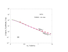
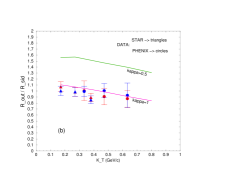
Figure 23: Part (a) shows the prediction for the spectrum based on the Tamale model. The points are from the minimum bias data from PHENIX Collaboration. The emissivity $\kappa$ is indicated in each curve. Part (b) shows results for the ratio $R_{out}/R_{sid}$ for our model and for two values of the emissivity. The ratio corresponding to $\kappa=1$ agrees very well with the PHENIX data points, within the experimental error bars but the one with 50% emissivity is completely excluded by data. The plots were extracted from Ref.sspqm02 .

Table 4 illustrates the time variables for two different assumptions on the emissivity, $\kappa$. I also write the estimated fraction of the particles emitted from the surface during the period $\tau_{0}\leq\tau\leq\tau_{f}$, ${\cal S}/{\cal N}_{tot}$, relative to the total number of produced particles, ${\cal N}_{tot}$, as well as the remnant portion at freeze-out, ${\cal V}$$/{\cal N}_{tot}$, then emitted from the entire volume. With the above parameters, we estimated the spectra and compared with experimental data from RHIC/Phenix Collaborationphenix , restricted to the central rapidity region. This is shown in Fig. 23.

With this model we managed to roughly explain the trend of data for $R_{out}$ but failed for $R_{sid}$, since it was independent on $K_{T}$. This, however, was expected, since the flow was neglected. The ratio, however, as can be seen from Fig. 23, came up just right, through the middle of the data pointssspqm02 ! Nevertheless, only much afterwards we did realize our emissivity parameter, $\kappa$, which controlled the surface emission, differed from the conventional one associated to a black-body. In fact, only by then we realized that the system would have to irradiate about four times more than an usual black-body for matching the data points. We then concluded that it was another strong evidence that flow should be included in the estimates, which is still under investigation.

II.15 II.9.2  IC, SPheRio, CEM & HBT

In Ref.sghk , Otávio, Frédérique, Yogiro and Takeshi analyze the effects of fluctuations in the initial conditions (IC), and of the continuous emission (CE) model, in two-pion interferometry within the hydrodynamical description of the SPheRio codespherio , comparing the results with the RHIC/STAR data.

The IC are, for simplicity, usually chosen as highly symmetric and smooth distributions of velocities and thermodynamical quantities. These IC correspond to mean distributions of hydrodynamical variables, averaged over several events. Nevertheless, for the typical finite systems formed in high energy collisions, large fluctuations are expected, varying from event to event. Moreover, the IC on the event-by-event basis often show small high-density spotssghk in the energy distribution. Being so, it would be expected that such spots would manifest themselves in the particle emission, contributing to decrease the HBT radii. In order to produce event-by-event fluctuating IC, in Ref.sghk they used the NeXus event generatornexus : once the incident nuclei and incident energy are given, it produces the energy-momentum tensor distribution at the proper time $\sqrt{t^{2}-z^{2}}$, in an event-by-event basis. This, together with the baryon-number density distributions constitute the fluctuating IC. No strangeness was introduced in the calculation.

On the other hand, the CE model we already discussed in Sec. II.5, is a alternative picture for describing the final state of the high energy collisions, i.e., the particle emission. According to the CE model, this emission occurs not only from the sharply defined freeze-out surface but also happens continuously, from the whole expanding volume at different temperatures and times. The main ingredients of the model are discussed in more detail by Frédérique Grassi in her review, in this volume. The basic formulation for CE interferometry was discussed in Sec. II.5.

In between the assumptions in the IC and the final stages described by the CE picture, there is the system evolution. This is considered in Ref.sghk by means of hydrodynamics, developed in the code SPheRio, which was based on the Smoothed Particle Hydrodynamics (SPH), first used in astrophysics and more recently adapted to nuclear collisionsspherio . SPH uses discrete Lagrangian coordinates attached to small volumes (“particles”) with some conserved quantities, which they take as the entropy and baryon number. For details about SPheRio and hydrodynamics, see the review by Yogiro Hama and Takeshi Kodama, in this volume.

Some of the results shown in Ref.sghk are summarized in Fig. 24.

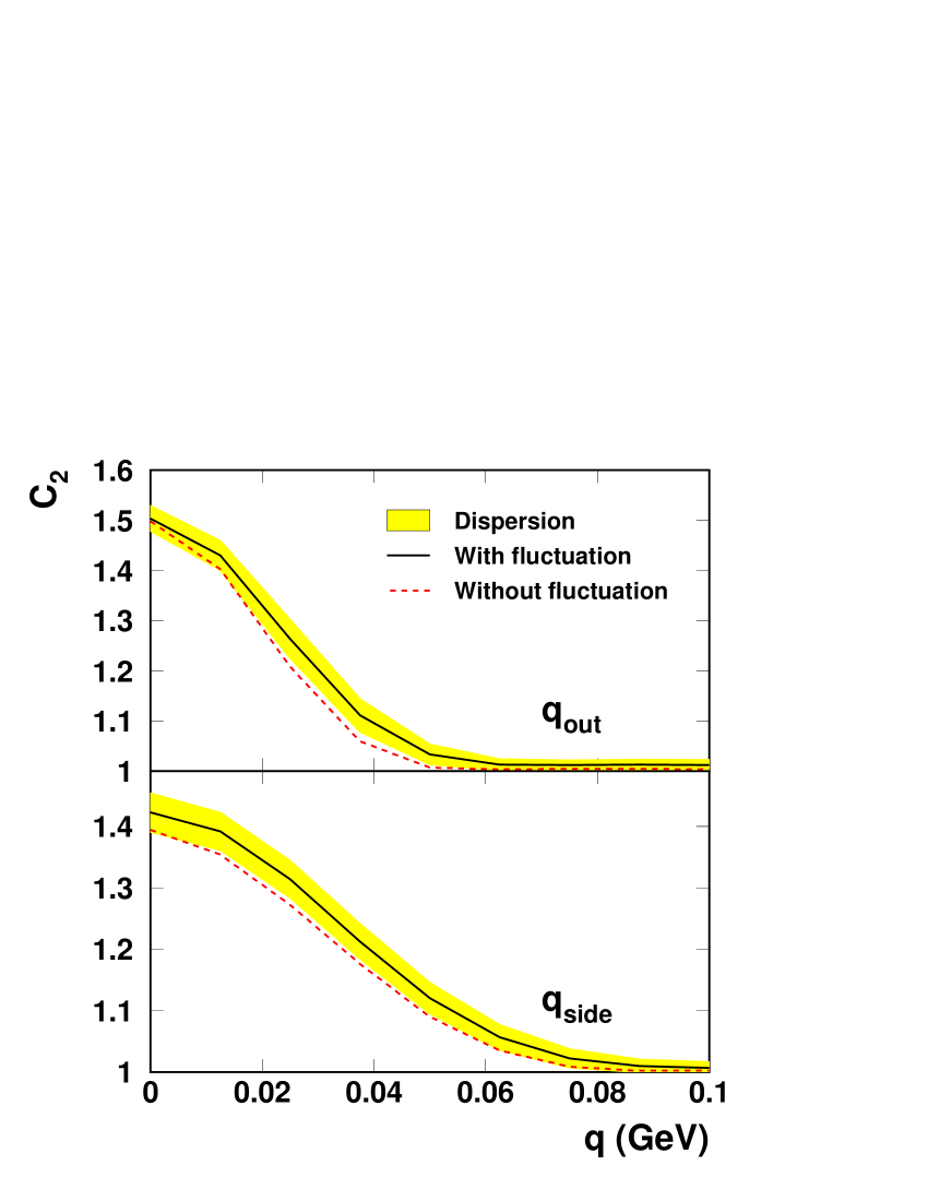
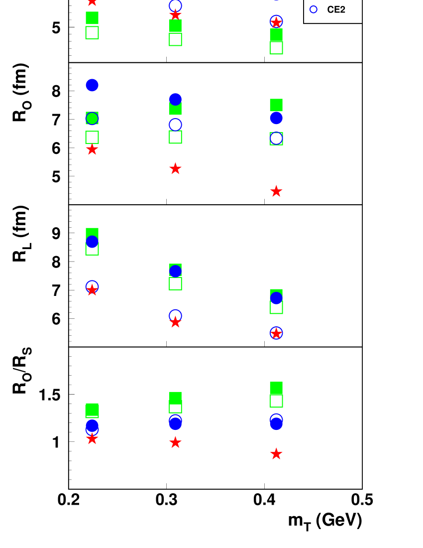
Figure 24: The plot on the left shows correlation functions assuming fluctuating IC and average IC, with sudden freeze-out. The $q_{O,S,L}$ that are not displayed in the horizontal axes were integrated in the interval $0\leq q_{O,S,L}\leq 35$ MeV. The plot on the right shows the radii $R_{O},R_{S},R_{L}$ together with the ratio $R_{O}/R_{S}$, as a function of $m_{T}$. The complement 1 stands for average IC and 2, for fluctuating IC. The plots were extracted from Ref.sghk .

To test the effect of fluctuations in the IC, a sudden freeze-out is initially assumed, at $T_{f.o.}=128$ MeV. In the left part of Fig. 24 the correlation function $C_{2}$, averaged over 15 fluctuating events, is compared with the corresponding $C_{2}$ with average IC (i.e., no fluctuations). The IC fluctuations are reflected in the fluctuations seen in the correlation functions. Averaging the correlations over the fluctuating range, we see that the resulting $C_{2}$ is broader than the correspondent ones computed with average IC. So, the effect of the IC fluctuations is to reduce the effective radii extracted from the correlation functions. Besides, the shapes of the resulting correlations with fluctuating IC and with smoothed average IC, are different. On the right-hand-side of Fig. 24, it is shown the $m_{T}$ dependence of the HBT radii. These were estimated by fitting Gaussians to $C_{2}$. Results based on the CE model, as well as RHIC data from STAR Collaborationstar are also included in that plot.

From Fig. 24, we see that joint effects of the smooth IC with sudden freeze-out make the $m_{T}$ dependence of the outwards radii, $R_{O}$, flat or slightly increasing. The fluctuating IC push the effective radii towards smaller values and flat $m_{T}$ dependence. Adding the CE hypothesis to the analysis, we also see from Fig. 24 that all effective radii, $R_{O}$, $R_{S}$, and $R_{L}$ decrease with increasing $m_{T}$. This is expected, since in the CE picture, high-$k_{T}$ particles have a bigger chance of being emitted at early times, when the system is hot, mostly from its surface. On the contrary, low-$k_{T}$ particles are emitted later, when the system has already cooled down and has larger size due to the expansion. The role of the fluctuating IC in the CE case is mostly of reducing the values of the effective radii, without significantly changing its $m_{T}$ dependence. These two effects together improve the description of the data points, as seen in Fig. 24. Nevertheless, the ratio $R_{O}/R_{S}$ is still above unity and does not describe the data points yet. Another ingredient may still be lacking.

II.16 II.10  BACK-TO-BACK CORRELATIONS

The Back-to-Back Correlations (BBC) have a much more recent history. Under the historical perspective we are pursuing in this review, it is worthy to briefly revise its origin. In 1991, Andreev, Plümber and Weinerbbcapw wrote a paper in which they pointed out the surprise existence of a new quantum statistical correlation, among particle-antiparticle pairs. Thus, $\pi^{+}\pi^{-}$ correlations of this type would be similar to $\pi^{0}\pi^{0}$ (since $\pi^{0}$ is its own antiparticle) but entirely different from the Bose-Einstein correlations we discussed in the previous sections. They were related to the expectation value of the annihilation (creator) operator, more specifically, $<\hat{a}^{(\dagger)}(k_{1})\hat{a}^{(\dagger)}(k_{2})>\neq 0$, analogous to what is observed in two-particle squeezing in optics, where the averages are estimated using a density matrix that contains squeezed states. Although not all they discussed was correct, they pointed out that $C(\pi^{+}\pi^{-})>1$ and $C(\pi^{0}\pi^{0})>1$, reflecting particle-antiparticle quantum statistical effects. Later, SinyukovYS94 , discussed a similar effect for $\pi^{+}\pi^{-}$ and $\pi^{0}\pi^{0}$ pairs, claiming that the effects would be due to inhomogeneities in the system, as opposite homogeneity regions in HBT, which comes from a hydrodynamical description of the system evolution. He used Wick’s theorem for expanding the two-particle inclusive distribution in terms of bilinear forms.

We can understand the origin of this effect in a simpler way in terms of creation and annihilation operators, in the $\pi^{0}$ case. For instance, the single-inclusive distribution is written as

$$N_{1}({\mathbf{k}}_{i})=\omega_{{\mathbf{k}}_{i}}\frac{d^{3}N}{d{\mathbf{k}}_{i}}=\omega_{{\mathbf{k}}_{i}}\langle\hat{a}^{\dagger}_{{\mathbf{k}}_{i}}\hat{a}_{{\mathbf{k}}_{i}}\rangle\;,$$ (98)

and, after the decomposition that follows from Wick’s theorem, the two-particle distribution is written as

$$N_{2}({\mathbf{k}}_{1},{\mathbf{k}}_{2})=\omega_{{\mathbf{k}}_{1}}\omega_{{\mathbf{k}}_{2}}\langle\hat{a}^{\dagger}_{{\mathbf{k}}_{1}}\hat{a}^{\dagger}_{{\mathbf{k}}_{2}}\hat{a}_{{\mathbf{k}}_{2}}\hat{a}_{{\mathbf{k}}_{1}}\rangle$$ (99)

$$= \omega_{{\mathbf{k}}_{1}}\omega_{{\mathbf{k}}_{1}}\{\langle\hat{a}^{\dagger}_{{\mathbf{k}}_{1}}\hat{a}_{{\mathbf{k}}_{1}}\rangle\langle\hat{a}^{\dagger}_{{\mathbf{k}}_{2}}\hat{a}_{{\mathbf{k}}_{2}}\rangle+\langle\hat{a}^{\dagger}_{{\mathbf{k}}_{1}}\hat{a}_{{\mathbf{k}}_{2}}\rangle\langle\hat{a}^{\dagger}_{{\mathbf{k}}_{2}}\hat{a}_{{\mathbf{k}}_{1}}\rangle$$

$$\hskip 5.69046pt+\hskip 5.69046pt\langle\hat{a}^{\dagger}_{{\mathbf{k}}_{1}}\hat{a}^{\dagger}_{{\mathbf{k}}_{2}}\rangle\langle\hat{a}_{{\mathbf{k}}_{1}}\hat{a}_{{\mathbf{k}}_{2}}\rangle\}\;.$$

In Eq. (99), the first term corresponds to the product of the two single-inclusive distributions, the second one gives rise to the Bose-Einstein identical particle correlation, reflecting the last position, just after particle emission. The third term, absent in the $\pi^{\pm}\pi^{\pm}$ case, is the responsible for the particle-antiparticle correlation. Under analogous conditions as HBT, this last term usually vanishes but is non zero if the Hamiltonian of the system is of the type $H=H_{0}+H_{1}$, where $H_{0}$ is the free part in the vacuum (final particles) and $H_{1}$ represents the interaction of quasi-particles, resulting in an effective shift of their masses. Alternatively, as in the pioneer work in Ref. bbcapw , this could be similar to having a chaotic superposition of coherent states and the density matrix containing squeezed states.

Later, Andreev and Weinerandwei continued the discussion. They considered that, in high energy collisions, a pion blob (strongly interacting pion system, seen as a liquid) is formed and later undergoes a sudden freeze-out, where the pionic system (having background and excited states) is rapidly converted into free pions. They postulate that, at the moment of transition, they can relate in-medium creation and annihilation operators ($\hat{b}^{\dagger},\hat{b}$) to the corresponding free ones ($\hat{a}^{\dagger},\hat{a}$), by means of a squeezing transformation, with a real squeezing parameter [$r=\frac{1}{2}\ln(E_{fr}/E_{in})$]. In the same year, Asakawa and Csörgő proposed a similar structure to this previous approach, but relating in-medium operators to free ones by means of a Bogoliubov transformation. They suggested that, while the in-medium Hamiltonian, $H_{1}$, is diagonalized in terms of $\hat{b}^{\dagger},\hat{b}$, the free one is diagonalized by $\hat{a}^{\dagger},\hat{a}$. They also proposed to observe hadron mass modification in hot medium by means of Back-to-Back Correlations. However, the theory was not yet completely correct.

There were a few more tentative works by the two groups but the correct approach was finally written in 1999, by Asakawa, Csörgő, and Gyulassyacg .

The formalism developed for the case of an infinite medium can be summarized as follows. The in-medium Hamiltonian is written as ${H}=H_{0}-\frac{1}{2}\int d{\mathbf{x}}~{}d{\mathbf{y}}\phi({\mathbf{x}})\delta M^{2}({\mathbf{x}}-{\mathbf{y}})\phi({\mathbf{y}}),\;\;$where $H_{0}=\frac{1}{2}\int d{\mathbf{x}}\left(\dot{\phi}^{2}+|\nabla\phi|^{2}+m^{2}\phi^{2}\right),\;$is the asymptotic (i.e., free) Hamiltonian, in the rest frame of matter. The scalar field $\phi({\mathbf{x}})$ in the Hamiltonian $H$ corresponds to quasi - particles that propagate with a momentum-dependent medium-modified effective mass, which is related to the vacuum mass, $m$, via

$$m_{*}^{2}({|{\mathbf{k}}|})=m^{2}-\delta M^{2}({|{\mathbf{k}}|}).$$

The mass-shift is assumed to be limited to long wavelength collective modes: $\delta M^{2}({|{\mathbf{k}}|})\ll m^{2}$ if $|{\mathbf{k}}|>\Lambda_{s}$. Given such a mass shift, the dispersion relation is modified to $\Omega_{\mathbf{k}}^{2}=\omega^{2}_{\mathbf{k}}-\delta M^{2}(|{\mathbf{k}}|)$, where $\Omega_{\mathbf{k}}$ is the frequency of the in-medium mode with momentum ${\mathbf{k}}$.

The in-medium, thermalized annihilation (creation) operator is denoted by $b_{\mathbf{k}}$ ($b^{\dagger}_{\mathbf{k}}$), whereas the corresponding asymptotic operator for the observed quantum with four-momentum $k^{\mu}\,=\,(\omega_{\mathbf{k}},{\mathbf{k}})$, $\omega_{\mathbf{k}}^{2}=m^{2}+{\mathbf{k}}^{2}$ ($\omega_{\mathbf{k}}>0$) is denoted by $a_{\mathbf{k}}$ ($a^{\dagger}_{\mathbf{k}}$). These operators are related by the Bogoliubov transformation, i.e., $a_{{\mathbf{k}}_{1}}=c_{{\mathbf{k}}_{1}}b_{{\mathbf{k}}_{1}}+s^{*}_{-{\mathbf{k}}_{1}}b^{\dagger}_{-{\mathbf{k}}_{1}}$, which is equivalent to a squeezing operation. For this reason, $r_{\mathbf{k}}$ is called mode-dependent squeezing parameter. Note that the relative and the average pair momentum coordinates are $q^{0}_{1,2}=\omega_{1}-\omega_{2},$ ${\mathbf{q}}_{1,2}={\mathbf{k}}_{1}-{\mathbf{k}}_{2}$, $E_{i,j}=\frac{1}{2}(\omega_{i}+\omega_{j})$, and ${\mathbf{K}}_{1,2}=(1/2)({\mathbf{k}}_{1}+{\mathbf{k}}_{2})$. For shortening the notation, we wrote the squeezed functions as $c_{i,j}=\cosh[r({i,j},x)]$ and $s_{i,j}=\sinh[r({i,j},x)]$, where

$$r(i,j,x) = \frac{1}{2}\log\left[(K^{\mu}_{i,j}u_{\mu}(x))/(K^{*\nu}_{i,j}(x)u_{\nu}(x))\right]$$ (100)

$$= \frac{1}{2}\log\left[\frac{\omega_{k_{i}}(x)+\omega_{k_{j}}(x)}{\Omega_{k_{i}}(x)+\Omega_{k_{j}}(x)}\right].$$

Also, $n_{i,j}$ is the density distribution, which is taken as the Boltzmann limit of the Bose-Einstein distribution, i.e., $n^{(*)}_{i,j}(x)\approx\exp{\{-[K^{(*)^{\mu}}_{i,j}u_{\mu}(x)-\mu(x)]/T(x)\}}$, where the symbol ^∗ implies the use of in-medium mass, whereas it should be dropped where there is no mass-shift.

In cases where the boson is its own anti-particle, as for $\pi^{0}\pi^{0}$ or $\phi\phi$ correlations, the full correlation function consists of a HBT part (related to the chaotic amplitude, $G_{c}(1,2)$) together with a BBC portion (related to the squeezed amplitude, $G_{s}(1,2)$), as shown below

$$C_{2}({\mathbf{k}}_{1},{\mathbf{k}}_{2})=\frac{N_{2}({\mathbf{k}}_{1},{\mathbf{k}}_{2})}{N_{1}({\mathbf{k}}_{1})N_{1}({\mathbf{k}}_{2})}$$

$$=1+\frac{|G_{c}(1,2)|^{2}}{G_{c}(1,1)G_{c}(2,2)}+\frac{|G_{s}(1,2)|^{2}}{G_{c}(1,1)G_{c}(2,2)},$$ (101)

being the invariant single-particle and two-particle momentum distributions given by

$$G_{c}(1,2) = \sqrt{\omega_{{\mathbf{k}}_{1}}\omega_{{\mathbf{k}}_{2}}}\langle\hat{a}^{\dagger}_{{\mathbf{k}}_{1}}\hat{a}_{{\mathbf{k}}_{2}}\rangle,$$

$$G_{s}(1,2) = \sqrt{\omega_{{\mathbf{k}}_{1}}\omega_{{\mathbf{k}}_{2}}}\langle\hat{a}_{{\mathbf{k}}_{1}}\hat{a}_{{\mathbf{k}}_{2}}\rangle,$$

$$G_{c}(i,i) = G_{c}(k_{i},k_{i})=N_{1}({\mathbf{k}}_{i}).$$ (102)

So far, the derivation considered an infinite system. The effects of finite size on BBC will be considered afterwards in the text. In Ref.acg , they discussed the influence of finite emission times, observing that the BBC in this case was suppressed when compared to the instant emission. Including the finite emission time as $\theta(t-t_{0})\Gamma\exp[-\Gamma(t-t_{0})]$, $C_{2}({\mathbf{k}}_{1},{\mathbf{k}}_{2})-1$ acquires a multiplicative factor $[1+(\omega_{\mathbf{k}}-\omega_{-\mathbf{k}})^{2}/\Gamma^{2}]$. They illustrated the maximum BBC, corresponding to $C_{2}({\mathbf{k}},-{\mathbf{k}})$ for the $\phi$-meson, obtaining a considerable magnitude for the BBC correlation function, in spite of considering the time suppression. We will see this more explicitly later.

As we discussed in the beginning of this section, the BBC is a different type of correlation, discovered for boson-antiboson pairs. More recently, Tamás Csörgő, Yogiro Hama, Gastão Krein, Prafulla K. Panda, and myself demonstrated that a similar correlation existed between fermion-antifermion pairs, if the mass of the fermions were modified in a thermalized medium. We already saw in the Introduction that, regarding the HBT effect, identical bosons have an opposite behavior as compared to identical fermions, as illustrated in Fig. 4, where we see that quantum statistics suppresses the probability of observing pairs of identical fermions with nearby momenta, while it enhances such a probability in the case of bosons. With respect to BBC, however, we found out a very different situation: fermionic BBC are positive and similar in strength to bosonic BBC! And, contrary to the HBT correlations, the BBC are unlimited.

In the fermion BBC case, there are expressions similar to Eq.(98) and (99),

$$N_{1}({\mathbf{k}}_{i})=\omega_{{\mathbf{k}}_{i}}\langle a^{\dagger}_{{\mathbf{k}}_{i}}a_{{\mathbf{k}}_{i}}\rangle\;\;;\;\;\tilde{N}_{1}({\mathbf{k}}_{i})=\omega_{{\mathbf{k}}_{i}}\langle\tilde{a}^{\dagger}_{{\mathbf{k}}_{i}}\tilde{a}_{{\mathbf{k}}_{i}}\rangle\;,$$ (103)

$$N_{2}({\mathbf{k}}_{1},{\mathbf{k}}_{2})=\omega_{{\mathbf{k}}_{1}}\omega_{{\mathbf{k}}_{2}}\langle a^{\dagger}_{{\mathbf{k}}_{1}}\tilde{a}^{\dagger}_{{\mathbf{k}}_{2}}\tilde{a}_{{\mathbf{k}}_{2}}a_{{\mathbf{k}}_{1}}\rangle\;.$$ (104)

In the above expressions,$<\hat{O}>$ denotes the expectation value of the operator $\hat{O}$ in the thermalized medium and $a^{\dagger},a,\tilde{a}^{\dagger},\tilde{a}$ are, respectively, creation and annihilation operators of the free baryons and antibaryons of mass $M$ and $\omega_{k}=\sqrt{M^{2}+|\vec{k}^{2}|}$, which are defined through the expansion of the baryon field operator as $\Psi(\vec{x})=\frac{1}{V}\sum_{\lambda,\lambda^{\prime},\vec{k}}(u_{\lambda,\vec{k}}a_{\lambda,\vec{k}}+v_{\lambda^{\prime},-\vec{k}}a^{\dagger}_{\lambda^{\prime},-\vec{k}})e^{i\vec{k}.\vec{x}}$; $V$ is the volume of the system, $u_{\lambda,\vec{k}}$ and $v_{\lambda^{\prime},-\vec{k}}$ are the Dirac spinors, where the spin projections are $\lambda,\lambda^{\prime}=1/2,-1/2$. The in-medium creation and annihilation operators are denoted by $b^{\dagger},b,\tilde{b}^{\dagger},\tilde{b}$. While the $a$-quanta are observed as asymptotic states, the $b$-quanta are the ones thermalized in the medium. They are related by a fermionic Bogoliubov-Valatin transformation,

$$\left(\begin{array}[]{c}a_{\lambda,{\mathbf{k}}}\\ \tilde{a}^{\dagger}_{\lambda^{\prime},-{\mathbf{k}}}\end{array}\right)=\left(\begin{array}[]{cc}c_{\mathbf{k}}&\frac{f_{\mathbf{k}}}{|f_{\mathbf{k}}|}\,s_{\mathbf{k}}\,A\\ -\frac{f^{*}_{\mathbf{k}}}{|f_{\mathbf{k}}|}\,s^{*}_{\mathbf{k}}\,A^{\dagger}&c^{*}_{\mathbf{k}}\end{array}\right)\left(\begin{array}[]{c}b_{\lambda,{\mathbf{k}}}\\ \tilde{b}^{\dagger}_{\lambda^{\prime},-{\mathbf{k}}}\end{array}\right),$$ (105)

here $c_{1}=\cos r_{1}$, $s_{1}=\sin r_{1}$, and

$$\tan(2r_{1})=-\frac{|{\bf k}_{1}|\Delta M({\bf k}_{1})}{\omega({\bf k}_{1})^{2}-M\Delta M({\bf k}_{1})}$$ (106)

is the fermionic squeezing parameter. Note that in the fermionic case, the squeezing parameter is the coefficient of sine and cosine functions, differently than the bosonic cases in which appeared their hyperbolic counterparts. In Eq. (105) $A$ is a $2~{}\times~{}2$ matrix with elements $A_{\lambda_{1}\lambda_{2}}=\chi^{\dagger}_{\lambda_{1}}\sigma\cdot{\hat{\bf k}}_{1}\tilde{\chi}^{\phantom{\dagger}}_{\lambda_{2}}$, where $\hat{\bf k}_{1}={\bf k}_{1}/|{\bf k}_{1}|$, $\chi$ is a Pauli spinor and $\tilde{\chi}=-i\sigma^{2}\chi$. Since $r$ is real in the present case, we drop the complex-conjugate notation in what follows.

In order to evaluate the thermal averages above, the system is modelled as a globally thermalized gas o quasi-particles (quasi-baryons). In this description, the medium effects are taken into account through a self-energy function, which, for a spin-$\frac{1}{2}$ particle (we will focus on proton and anti-proton pairs), under the influence of mean fields in a many-body system, can be written as $\Sigma=\Sigma^{s}+\gamma^{0}\Sigma^{0}+\gamma^{i}\Sigma^{i}$. In this expression, $\Sigma^{0}$ is a weakly momentum-dependent function which, for locally thermalized systems that we are considering, has the role of shifting the chemical potential, i.e., $\mu_{*}=\mu-\Sigma^{0}$. The vector part is very small and is neglected. The scalar part can be written as $\Sigma^{s}=\Delta M({\bf k})$. With these approximations we describe the system with a momentum-dependent in-medium mass, $M_{*}({\bf k})=M-\Delta M(|{\bf k}|)$.

We are mainly interested here in the study of the squeezed correlation function, which corresponds to considering only the joint contribution of the first and third terms on the rhs of Eq. (101). In the fermionic case and for an infinite, homogeneous thermalized medium, the correlation BBC part of the correlation function is written as

$$\!\!\!\!\!\!\!\!\!\!\!\!C_{2}^{(+-)}({\bf k}_{1},-{\bf k}_{1})=1+\;[1+(2\Delta t\;\omega_{\bf k})^{2}]^{-1}\;\times$$

$$\!\!\!\!\!\!\!\!\!\!\!\!\{\frac{(1-n_{\bf k}-\tilde{n}_{\bf k})^{2}(c_{\bf k}s_{\bf k})^{2}}{\left[c_{\bf k}^{2}n_{\bf k}+s_{\bf k}^{2}(1-\tilde{n}_{\bf k})\right]\left[c_{\bf k}^{2}\tilde{n}_{\bf k}+s_{\bf k}^{2}(1-n_{\bf k})\right]}\},\;$$ (107)

where $n_{\bf k}=\frac{1}{\exp\left[(\Omega_{\bf k}-\mu_{*})/T\right]+1}\;;\;\tilde{n}_{\bf k}=\frac{1}{\exp\left[(\Omega_{\bf k}+\mu_{*})/T\right]+1}$ in terms of which the net baryonic density is written as $\rho_{B}=(g/V)\sum_{\bf k}~{}\bigl{(}n_{\bf k}-n_{-{\bf k}}\bigr{)}$. In Eq. (107) we have included a more gradual freeze-out by means of a finite emission interval, similarly to what was done in Refacg , which has the effect of suppressing the BBC signal.

For our numerical study of the fermionic back-to-back correlations (fBBC), we considered, for simplicity, momentum independent in-medium masses, i.e., $M_{*}=M-\Delta M$. There is no difficulty in considering momentum dependent self-energies, however, this requires the commitment to a specific model and we preferred to leave it for a future investigation. In Fig. 25 we show fBBC for $\bar{p}p$ pairs as a function of the in-medium mass $M_{*}$, for three values of the net baryonic density $\rho_{B}$: for the normal nuclear matter, one tenth of this value and for the baryon free region, i.e., $\rho_{B}=0$. We show in the same plot results for the bosonic case, bBBC, corresponding to $\phi$ meson pair, whose mass is close to the proton mass and was the example used in Ref.acg .

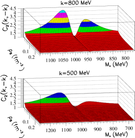
Figure 25: The plot on the left shows back-to-back correlations of $\bar{p}p$ (fBBC) and of $\phi$-meson pairs, for $|\vec{k}|=800$ MeV/c. The plot on the right shows the dependence of the fBBC on the in-medium modified proton mass, $M_{*}$, and on the net baryon density, $\rho_{B}$ and two typical values of $|\vec{k}|$. In both cases $T=140$ MeV and $\Delta t=2$ fm/c. The plots were extracted from Ref.pchkp .

We see from Fig. 25 that fBBC and bBBC are, indeed, both positive correlations, with similar shape, and of the same order of magnitude. We also observe that fBBC is strongly enhanced for decreasing net baryonic density, being maximal for $\rho_{B}\approx 0$, i.e., for approximately equal baryon and anti-baryon densities. Fig. 25 also shows that fBBC increases with increasing momentum. Besides, we see that the shape of fBBC is very sensitive to the shape of the freeze-out distribution and, in the limit of a very long freeze-out, both fBBC and bBBC would vanish.

So far, we considered an infinite and homogeneous medium, although we know that the systems produced in high energy collisions, including the ones at RHIC, have finite sizes. Thus, we need to know if the BBC signal would survive when more realistic spacial and dynamical considerations were made. For pursuing this purpose, we studied the effects on the squeezing parameter and on the back-to-back correlation of a finite size medium moving with collective velocity. For this, we considered a hydrodynamical ensemble, in which the amplitudes $G_{c}$ and $G_{s}$ in Eq. (101) and (102) are extended to the special form derived by Makhlin and Sinyukov sm .

$$G_{c}(1,2) = \frac{1}{(2\pi)^{3}}\int d^{4}\sigma_{\mu}(x)K_{1,2}^{\mu}e^{iq_{1,2}\cdot x}\{|c_{1,2}|^{2}n_{1,2}$$ (108)

$$\hskip 28.45274pt+\;\;\;|s_{-1,-2}|^{2}(n_{-1,-2}+1)\},$$

$$G_{s}(1,2)\!\! = \!\!\frac{1}{(2\pi)^{3}}\int d^{4}\sigma_{\mu}(x)K_{1,2}^{\mu}e^{2iK_{1,2}\cdot x}\{s^{*}_{-1,2}c_{2,-1}n_{-1,2}$$ (109)

$$\hskip 28.45274pt+\;\;\;c_{1,-2}s^{*}_{-2,1}(n_{1,-2}+1)\}.$$

In Eq.(108) and (109) $d^{4}\sigma^{\mu}(x)=d^{3}\Sigma^{\mu}(x;\tau_{f})\,F(\tau_{f})d\tau_{f}$ is the product of the normal-oriented volume element depending parametrically on $\tau_{f}$ (the freeze-out hyper-surface parameter) and on the invariant distribution of that parameter $F(\tau_{f})$. We consider two possibilities: i) an instant freeze-out, corresponding to $F(\tau)=\delta(\tau-\tau_{0})$; ii) an extended freeze-out, with a finite emission interval, with $F(\tau)=[\theta(\tau-\tau_{0})/\Delta t]e^{-(\tau-\tau_{0})/\Delta t}$. These cases lead, after performing the integration in $d\tau$ in Eq. (108) and (109) with weight ($E_{i,j}\;e^{-i2E_{i,j}\tau}$), respectively to: i) $(\omega_{i}+\omega_{j})\;e^{-i(\omega_{i}+\omega_{j})\tau_{0}}$; ii) $(\omega_{i}+\omega_{j})[1+[(\omega_{i}+\omega_{j})\Delta t]^{-2}$.

According to the hydrodynamical solution, we can express the chemical potential as $\frac{\mu(x)}{T(x)}=\frac{\mu_{0}}{T}-\frac{{\mathbf{r}}^{2}}{2R^{2}}$, being $R$ the radius of the system, $T=T(x)$ the temperature of the system in each space-time point $x$, and $\mu_{0}$ a constant. We assume that the system expands with four-dimensional flow velocity $u^{\mu}=\gamma(1,{\mathbf{v}})$, where ${\mathbf{v}}=<\!\!u\!\!>\!\frac{\mathbf{r}}{R}$. In the non-relativistic limit, we can write $\gamma=(1+{\mathbf{v}})^{-1/2}\approx 1+\frac{1}{2}{\mathbf{v}}^{2}$, thus taking into account all terms up to ${\cal O}(mv^{2})$. We estimate the geometrical and dynamical effects on the BBC in the bosonic case, considering the in-medium changes for the $\phi$-meson.

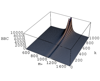
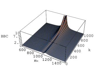
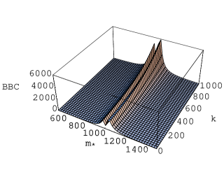
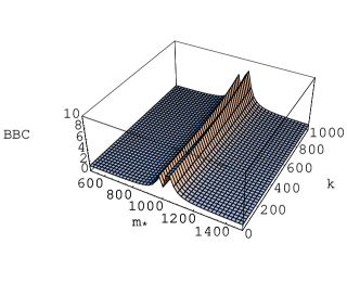
Figure 26: The Back-to-Back Correlation is shown as a function of the pair average momentum, for ${\mathbf{k}}_{1}=-{\mathbf{k}}_{2}={\mathbf{k}}$, when considering the values of the shifted mass around the vacuum mass, $m_{\phi}=1020$ MeV). The squeezed mass was considered to change in the entire Gaussian volume, with rms $R=6$ fm. In the top plots no flow was included, i.e., ${\mathbf{v}}=<\!\!u\!\!>\!\frac{\mathbf{r}}{R}=0$, but radial flow with $<\!\!u\!\!>\!=0.5$ was included in the bottom cases. Plots on the left side correspond to the case of particles emitted instantly, and those on the right, to the case where particles are emitted during a finite time interval, $\Delta t$.

For small mass shifts, i.e. $\frac{(m-m_{*})}{m}\ll 1$, the flow effects on the squeezing parameter are of fourth order, i.e., ${\cal O}\left(\frac{Kin.\;energy}{m}\right)(\frac{\delta m^{2}}{m^{2}})$. As a consequence, the flow effects on $r_{i,j}$ can be neglected, and the factor $c_{i,j}$ and $s_{i,j}$ become flow independent, although they could still depend on the coordinate $r$ through the shifted mass, $m_{*}$ (e.g., through $T(x)$, as in hydrodynamics), which is not considered here.

For the sake of simplicity, trying to keep the results as much analytical as possible (for details, see chkppflow ), we make the hypothesis that the mass-shift is independent on the position within the fireball. We further assume that this last one has a sharp surface, i.e., $\delta m=0$ on the surface, and also the density vanishes outside the system volume. The spatial integration in Eq. (108) and (109) extends over the region where the mass-shift is non-vanishing, which is not infinitely large. For instance,I in relativistic heavy ion collisions is a finite region $V\approx R^{3}\approx(5-10)^{3}$ fm³. We should keep in mind that the vacuum term in the integrand vanishes outside the mass-shift region, since it is proportional to $s_{i,j}$, which vanishes in that region. On the other hand, the terms proportional to $n^{(*)}_{i,j}(x)$ are finite. Being so, we can extend the integration in Eq. (108) and (109) to infinity and, without much loss of generality, we can choose for $V$ a Gaussian profile, $\exp[-{\mathbf{r}}^{2}/(2R^{2})]$.

We studied the flow effects in two cases. The first one considers the mass-shift as occurring in the entire volume of the system, for which the parameter $R$, in the exponential, represents the cross-sectional area of the Gaussian profile with rms $R$ . The other case corresponds to considering the shift of mass in a smaller volume, associated to a certain $R_{s}<R$. We show in Fig. 26 the results for the first case only, where we adopted $R=6$ fm. The BBC signals for the mass shift in the partial volume, although not shown, are very similar to the ones in Fig. 26, except for the maximum strength of the bBBC signal, which is smaller than seen in the plots of Fig. 26, emphasizing that the effect is directly proportional to the size of the region where the mass-shift occurs. By comparing the top panels (no flow) with the bottom ones ($<\!\!u\!\!>\!=0.5$) in Fig. 26, we see that the flow has a suppression effect on the bBBC strength in the high momentum region. However, the presence of flow surprisingly enhances the BBC signal in the low momentum region (i.e., for $|{\mathbf{k}}|\lesssim 1000$ MeV), as compared to the no-flow case on top panel, suggesting this as the region to focus the search for the BBC effect. In any case, we conclude with enthusiasm that the BBC signal survives more realistic conditions, like finite sizes, time spread, and flow. This strongly encourages us to analyze even more realistic systems than the ones discussed here, and to optimize the way we should look for this interesting, although not yet observed, effect.

III BRIEF CONCLUDING REMARKS

I would like to finalize by emphasizing that, although a lot was written above about the evolution and contributions related to HBT, since its discovery about half a century ago, the present text merely covers a tiny fraction of what has been produced on this subject. An increasing number of people over these five decades have given countelss contributions to the field. Unfortunately, the lack of space would not allow me to mention and discuss them all. Finally, I would like to dedicate this review to the memory of my father, who passed away this year, as well as to Robert Hanbury-Brown and Richard Q. Twiss, on celebrating the 50^th anniversary of their first publication on this fabulous method and discovery.

I would like to express my gratitude to Yogiro Hama and Takeshi Kodama for devising, 15 years ago, and organizing ever since, this active group working on hadronic and nuclear interactions at high energies.

This work was partially supported by CNPq (Proc. Proc. N${}^{\b{o}}200410/82-2$) and Fundação de Amparo à Pesquisa do Estado de São Paulo (FAPESP), Projetos Temáticos $90/4074-5,93/2463-2,95/4635-0,98/2249-4$ and $00/04422-7$.

References

- (1) G. Goldhaber, Proc. Int. Workshop on Correlations and Multiparticle production (CAMP - LESIP IV), p. 409, ed. by M. Plümer, S. Raha, and R. M. Weiner, World Scientific (1991).
- (2) R.Hanbury-Brown and R. Q. Twiss, Phil. Mag. 45 (1954) 663, Nature 177 (1956) 26, Nature 178 (1956) 1447.
- (3) E. M. Purcell, Nature 178 (1956) 1449.
- (4) G. Goldhaber et al., Phys. Rev. 120 (1960) 300.
- (5) E. A. Bartnik and K. Rza̧ewski, Phys. Rev. D18 (1978) 4308.
- (6) M. Deutschmann et al., CERN/EP/PHYS 78-1 (January, 1978).
- (7) Sandra S. Padula and M. Gyulassy, Nucl. Phys. A525 (1991) 339c.
- (8) V. G. Grishin, G. I. Kopylov and M. I. Podgoretskiĭ, Sov. J. Nucl. Phys., 13 (1971) 638, Sov. J. Nucl. Phys. 14 (1972) 335.
- (9) G. Cocconi, Phys. Lett. 49B (1974) 459.
- (10) Richard M. Weiner, Bose-Einstein Correlations in Particle and Nuclear Physics, John Wiley & Sons, 1997.
- (11) M. Gyulassy, S. K. Kaufmann, and L. W. Wilson, Phys. Rev. C20 (1979) 2267.
- (12) G. N. Fowler and R. M. Weiner, Phys. Lett. 70B (1977) 201; Phys. Rev. D17 (1978) 3118; G. N. Fowler, N. Stelteand R. M. Weiner, Nucl. PHys. A319 (1979)349.
- (13) P. Grassberger, Nucl. Phys. B120 (1977) 231.
- (14) G. Bertsch, Nucl. Phys. A498 (1989) 173c.
- (15) S. Chapman, P. Scotto, and U. Heinz , Phys.Rev.Lett. 74 (1995) 4400-4403
- (16) W. A. Zajc, Hadronic Multiparticle Production, World Scientific Press, P. Carruthers, ed. (1988).
- (17) D. H. Boal, C. K. Gelbke and B. K. Jennings, Rev. Mod. Phys. 62 (1990) 553.
- (18) C-Y. Wong, Introduction to High-Energy Heavy-Ion Collisions, World Scientific (1994).
- (19) Heinz, B. Tomasik, U.. Heinz, B. Tomasik, U. A. Wiedermann and Y. F. Wu, Phys. Lett 382B (1996) 181.
- (20) T. Csörgő, Heavy Ion Phys. 15 (2002) 1-80.
- (21) C. Alder et al., STAR Collab., Phys. Rev. Lett. 87 (2001) 082301; K. Adcox et al, PHENIX Collab., Phys. Rev. Lett. 88 (2002) 192302.
- (22) Sandra S. Padula, Correlação entre Bosons Idênticos produzidos em Colisões Hadrônicas a Altas Energias, Ph.D. Thesis presented at Instituto de Física, Universidade de São Paulo (October 16, 1987).
- (23) J. D. Bjorken, private communication.
- (24) T. Åkesson et al., Phys. Let. 129B (1983) 269.
- (25) Y. Hama and Sandra S. Padula, Phys. Rev. D37 (1988) 3237.
- (26) L. D. Landau, Izv. Akad. Nauk SSSR Ser. Fiz. 17 (1953) 51; Collected Papers, p. 569 and 665, edited by D. Ter Haar (Gordon and Breach, 1967).
- (27) Y. Hama, Phys. Rev. D19 (1079 2623, Y. Hama and F. W. Pottag, Rev. Brtas. Fis 12 (1982) 247; Y. Hama and F. S. Navarra, PHys. Lett. 129B (1983) 251.
- (28) E. V. Shuryak, Phys. Lett. 44B (1973) 387.
- (29) S. Pratt, Phys. Rev. D33 (1986) 1314.
- (30) Miklos Gyulassy and Sandra S. Padula, Phys. Lett. 217B (1989) 181.
- (31) B. Andersson et al., Nucl. Phys. B281 (1987) 289; M. Gyulassy, CERN-TH. 4794 (1987), Proc. Eighth Balaton Conf. on Nucl. Phys. (ed. by Z. Fodor, KDKI, Budapest, 1987).
- (32) T. J. Humanic, Z. Phys. C38 (1988) 79; A. Bamberger et al., Phys. Lett. B203 (1988) 320.
- (33) . G. Bertsch, M. Gong, M. Tohyama, Phys. Rev. C37 (1988) 1896.
- (34) Sandra S. Padula and M. Gyulassy, Proc. Quark Matter ’88, Nucl. Phys. A498 (1989) 555c.
- (35) K. Kolehmainen and M. Gyulassy, Phys. Lett. B180 (1986) 203.
- (36) J. D. Bjorken, Phys. Rev. D27 (1983) 140.
- (37) Sandra S. Padula and M. Gyulassy, Nucl. Phys. B339 (1990) 378.
- (38) Miklos Gyulassy and Sandra S. Padula, Phys. Rev. C41 (1990) R21.
- (39) K. Kulka and B.Lörstad, Z. Phys. C45 (1990) 581.
- (40) Sandra S. Padula, M. Gyulassy, Nucl. Phys. A544 (1992) 537c.
- (41) Sandra S. Padula, M. Gyulassy, S. Gavin, Nucl. Phys. B329 (1990) 357.
- (42) Sandra S. Padula and M. Gyulassy, Phys. Lett. B348 (1995) 303.
- (43) T. Abott et al. (E802 Collab.), Phys. Rev. Lett. 64 (1990) 847, ibidem 66 (1991) 1567; ibidem 69 (1992) 1030; R. J. Morse, Nucl. Phys. A525 (1991) 531c.
- (44) Sandra S. Padula and Cristiane G. Roldão, Phys. Rev. D58 (1998) 2907.
- (45) Y. Akiba et al. (E859 Collab.),Phys. Rev. Lett. 70 (1993) 1057, V. Cianciolo, Nucl. Phys. A590 (1995) 459c; O. E. Vossnack, Nucl. Phys. A566 (1994) 535c; V. Cianciolo, Ph.D Thesis presented to MIT (May/1994).
- (46) Y. Hama, T. Kodama, and Sandra S. Padula, Phys. Rev. A 56 (1997) 2233.
- (47) D.F. Gaitan and L.A. Crum, J. Acoust. Soc. Am., Supple. 1 87, S141 (1990), D.F. Gaitan, L.A. Crum, C.C. Curch and R.A.Roy, J. Acoust. Soc. Am. 91, 3166 (1992); Sonoluminescence, L.A. Crum, Physics Today, Sep. (1994).
- (48) Casimir Energy for a Spehrical Cavity in a Dielectric: Toward a Model for Sonoluminescence?, K.A. Milton, hep-th/9510091; C. Eberlein, Phys. Rev. A53, 2772 (1996); Sonoluminescence and the Heimlich Effect, A. Chodos, hep-ph/9604368.
- (49) R.Löfstedt, B.P. Barber and S.J. Putterman, Phys. Fluids A5, 2911 (1993); W.C. Moss, D.B. Clarke, J.W. White and D.A. Young, Phys. Lett. A211, 69 (1996); Sonoluminescence: Sound into Light, Seth Putterman, Scientific American Fev. (1995).
- (50) C. Slotta and U. Heinz, Phys. Lett. B391, 469 (1997).
- (51) F. Grassi, Y. Hama and T. Kodama, Phys. Lett B355 (1995) 9; Z. Phys. C73 (1996) 153.
- (52) F. Grassi, Y. Hama, Sandra S. Padula, and O. Socolowski, Phys. Reviw C62 (2000) 44940.
- (53) T. Csörgö, J. Zimanyi, Nucl. Phys. A527 (1991) 621c; S. Chapman, J. R. Nix and U. Heinz, Phys. Rev. C52 (1995) 2694; T. Csörgö and B. Lörstad, Nucl. Phys. A590 (1995) 465.
- (54) T. Alber et al., NA35 Collab., Z. PHys. C66 (1995) 77.
- (55) Q.H. Zhang and Sandra S. Padula, Phys. Rev. C62 (2000) 24902.
- (56) E. V. Shuryak, Phys. Rev. D 42, 1764 (1990).
- (57) M. G.-H. Mostafa and C.Y. Wong, Phys. Rev. C 51, 2135 (1995).
- (58) S. Sarkar, P. K. Roy, D. K. Srivastava, and B. Sinha, J. Phys. G22, 951 (1996)A. Ayala and A. Smerzi, Phys. Lett. B405, 20 (1997).
- (59) Yu. Sinyukov, Nucl. Phys. A566, 589c (1994).
- (60) O.W. Greenberg, Phys. Rev. Lett. 64, 705 (1990), and Phys. Rev. D43, 4111 (1991).
- (61) D. V. Anchishkin, A. M. Gavrilik and N. Z. Iorgov, Eur. Phys. J. A7 229 (2000); Mod. Phys. Lett A15 (2000) 1637.
- (62) Q. H. Zhang and Sandra S. Padula, Phys. Rev. C69 (2000) 24907.
- (63) S. S. Avancini and G. Krein, J. Phys. A: Math. Gen. 28, 685 (1995).
- (64) Sérgio M. Antunes, Estudo dos efeitos da estatística não extensiva de Tsallis em interferometria de pions, IFT-D.003/2000.
- (65) C. Tsallis, J. Stat. Phys. 52 (2988) 479.
- (66) . Büyükkili,̧ D. Dermirhan, A. Güle, Phys. Rev. A197 (1995) 209; Q.A.Wang and A.L. Méhauté, Phys.Lett, A 235, (1997) 222; U.Tirnakli, F. Büyükkili,̧ D.Dermirhan, Phys. Lett A 245, (1998) 62.
- (67) O.V.Utyuzh, G.Wilk, and Z.Włodarczyk, J. Phys. G26 (2000) L39.
- (68) S. Pratt, Phys. Rev. Lett. 53 (1984) 1219.
- (69) G. Kaniadakis, A. Lavagno, M.Lissia, P. Quarati, nucl-th/9812033.
- (70) W. M. Alberico, A. Lavagno, P. Quarati, Nucl. Phys. A680 (2000) 94.
- (71) Victor Viscarra-Ruiz, Estimativa da densidade de espaço-de-fase em colisões a altas energias usando interferometria, IFT-D.008/2000.
- (72) G. F. Bertsch, Phys. Rev. Lett. 71 (1994) 2349.
- (73) F. Laue, Proc. Quark Matter 2001, Nucl. Phys. A698 (2002) 177c; C. Alder et al., STAR Collab., Phys. Rev. Lett. 87 (2001) 082301.
- (74) K. Adcox et al, Phys. Rev. Lett. 88 (2002) 192302.
- (75) U. Heinz and P. Kolb, Nucl. Phys. A702, 269 (2002).
- (76) Sandra S. Padula, Nucl. Phys. A715 (2003) 637c.
- (77) O. Socolowski Jr., F. Grassi, Y. Hama, and T. Kodama, Phys. Rev. Lett. 93 (2004) 182301.
- (78) C.E. Aguiar, T. Kodama, T. Osada and Y. Hama, J. Phys. G27, 75 (2001).
- (79) H.J. Drescher et al., J. Phys. G25, L91 (1999); Nucl. Phys. A661, 604 (1999).
- (80) I. V. Andreev, M. Plümer and R. M Weiner, Phys. Rev. Lett. 67 (1991) 3475.
- (81) I. V. Andreev and R. M Weiner, Phys. Lett. B373 (1996) 159.
- (82) M. Asakawa and T. Csörgö, H. Ion Phys. 4 (1996) 233.
- (83) M. Asakawa, T. Csörgö, and M. Gyulassy, Phys. Rev. Lett. 83 (1999) 4013.
- (84) A. Makhlin and Yu. Sinyukov, Sov. J. Nucl. Phys. 46, (1987) 354; Yad. Phys. 46, (1987) 637; Yu. Sinyukov, Nucl. Phys. A566, (1994) 598c.
- (85) P.K. Panda, T. Csörgo, Y. Hama, G. Krein, S.S. Padula, Phys. Lett. B512 (2001) 49.
- (86) T. Csörgő, Y. Hama, G. Krein, Sandra S. Padula, P.K. Panda, in preparation.