Photoproduction of Pentaquark in Feynman and Regge Theories

Abstract

Photoproduction of the $\Theta^{+}$ pentaquark on the proton is analyzed by using an isobar and a Regge models. The difference in the calculated total cross section is found to be more than two orders of magnitude for a hadronic form factor cut-off $\Lambda>1$ GeV. Comparable results would be obtained for $0.6\leq\Lambda\leq 0.8$ GeV. We also calculate contribution of the $\Theta^{+}$ photoproduction to the GDH integral. By comparing with the current phenomenological calculation, it is found that the GDH sum rule favors the result obtained from Regge approach and isobar model with small $\Lambda$.

The observation of a narrow baryon state from the missing mass spectrum of $K^{+}n$ and $K^{+}p$ with extracted mass $M=1540$ MeV leps ; saphir ; clas ; diana ; hermes has led to a great excitement in hadronic and particle physics communities. This state is identified as the $\Theta^{+}$ pentaquark that has been previously predicted in the chiral soliton model diakonov . Since then a great number of investigation on the $\Theta^{+}$ production has been carried out. In general, these efforts can be divided into two categories, i.e., investigations using hadronic and electromagnetic processes. The electromagnetic production (also known as the photon-induced production) is, however, well known as a more ”clean” process, since electromagnetic interaction has been well under-controlled. Furthermore, photoproduction process provides an easier way to ”see” the $\Theta^{+}$ which contains an antiquark, since all required constituents are already present in the initial state Karliner:2004gr . Other processes, such as $e^{+}e^{-}$ and ${\bar{p}}p$ annihilations, would produce the strangeness-antistrangeness (and baryon-antibaryon in the case of $e^{+}e^{-}$) from gluons, which has a consequence of the suppressed cross section Titov:2004wt .

Several $\Theta^{+}$ photoproduction studies have been performed by using isobar models with Born approximation ysoh ; liu&ko2004 ; nam ; qzhao ; yu&ji2004 ; yrliu ; wwli ; pko , with the resulting cross section spans from several nanobarns to almost one $\mu$barn, depending on the $\Theta^{+}$ width, parity, hadronic form factor cut-off, and the exchanged particles used in the process. Those parameters are unfortunately still uncertain at present. Furthermore, the lack of information on coupling constants has severely restricted the number of exchanged particles used in the process, including a number of resonances which have been shown to play important roles at $W$ around 2 GeV and determine the shape of cross sections of the $K\Lambda$ and $K\Sigma$ photoproductions mart2000 .

Therefore, it is important to constrain the proliferation of models by using all available informations in order to achieve a reliable cross section prediction which is urgently required by present experiments. For this purpose we will exploit the isobar and Regge models and using all available coupling constant informations. The use of Regge model has a great advantage since the number of uncertain parameters is much less than those of the isobar one. Nevertheless, from the experience in $K\Lambda$ and $K\Sigma$ photoproduction, in spite of using a small number of parameters Regge model works quite well at high energies and the discrepancy with experimental data at the resonance region is found to be less than 50% guidal97 ; Mart:2003yb . Concerning with the high threshold energy of this process ($W\approx$ 2 GeV) it is naturally imperative to consider the Regge mechanism in the calculation. As an example, a reggeized isobar model has shown a great success in explaining experimental data of $\eta$ and $\eta^{\prime}$ photoproductions up to the photon lab energy $E_{\gamma}^{\rm lab}=2$ GeV Chiang:2002vq .

In this paper we compare the cross sections obtained from both models and investigate the effect of hadronic form factor cut-off ($\Lambda$) variation in the isobar model. To this end, we will consider the positive parity of $\Theta^{+}$, since previous calculations have found a ten times smaller cross section if one used the negative parity state, whereas we concern very much with the overprediction of cross sections by isobar models. Moreover, our first motivation is to investigate the effect of $\Lambda$ variation and compare the varied cross sections with that of the Regge model. To further support our finding, we will calculate contribution of the $\Theta^{+}$ photoproduction to the Gerasimov-Drell-Hearn (GDH) integral from both models. Since only GDH integral for proton is relatively well understood drechsel , we calculate only photoproduction on the proton

$$\gamma(k)+p(p)\longrightarrow{\bar{K}}^{0}(q)+\Theta^{+}(p^{\prime})~{}.$$

In isobar model the amplitudes are obtained from a series of tree-level Feynman diagrams shown in Fig. 1. They contain the $p$, $\Theta^{+}$, $K^{*}$ and $K_{1}$ intermediate states. The neutral kaon $K^{0}$ cannot contribute to this process since a real photon cannot interact with a neutral meson. The $K^{*}$ and $K_{1}$ intermediate states are considered here, since previous studies on $K\Lambda$ and $K\Sigma$ photoproductions have proven their significant roles. The transition matrix for both reactions can be decomposed into

$$M_{\mathrm{f}i} = {\bar{u}}({\mbox{\boldmath${p}$}}^{\prime})\sum_{i=1}^{4}A_{i}~{}M_{i}~{}u({\mbox{\boldmath${p}$}})~{},$$ (1)

where the gauge- and Lorentz invariant matrices $M_{i}$ are given in, e.g., Ref. Lee:1999kd . In terms of the Mandelstam variables $s$, $u$, and $t$, the functions $A_{i}$ are given by

$$A_{1} \!\!=\! -\frac{eg_{K\Theta N}F_{1}(s)}{s-m_{p}^{2}}\left(1+\kappa_{p}\frac{m_{p}-m_{\Theta}}{2m_{p}}\right)$$ (2)

$$-\frac{eg_{K\Theta N}F_{2}(u)}{u-m_{\Theta}^{2}+im_{\Theta}\Gamma_{\Theta}}\!\left[1+\frac{\kappa_{\Theta}\left(m_{\Theta}-m_{p}-{\textstyle\frac{i}{2}}\Gamma_{\Theta}\right)}{2m_{\Theta}}\right]$$

$$-\frac{G^{T}F_{3}(t)}{M(t-m_{K^{*}}^{2}+im_{K^{*}}\Gamma_{K^{*}})(m_{\Theta}+m_{p})}~{},$$

$$A_{2} = \frac{2eg_{K\Theta N}}{t-m_{K}^{2}}\left(\frac{1}{s-m_{p}^{2}}+\frac{1}{u-m_{\Theta}^{2}}\right){\widetilde{F}}(s,u,t)$$ (3)

$$+\frac{G^{T}_{K^{*}}F_{3}(t)}{M(t-m_{K^{*}}^{2}+im_{K^{*}}\Gamma_{K^{*}})(m_{\Theta}+m_{p})}$$

$$-\frac{G^{T}_{K_{1}}F_{3}(t)}{M(t-m_{K_{1}}^{2}+im_{K_{1}}\Gamma_{K_{1}})(m_{\Theta}+m_{p})},$$

$$A_{3} = \frac{eg_{K\Theta N}}{s-m_{p}^{2}}~{}\frac{\kappa_{p}F_{1}(s)}{2m_{p}}-\frac{eg_{K\Theta N}}{u-m_{\Theta}^{2}}~{}\frac{\kappa_{\Theta}F_{2}(u)}{2m_{\Theta}}$$

$$-\frac{G^{T}_{K^{*}}F_{3}(t)}{M(t-m_{K^{*}}^{2}+im_{K^{*}}\Gamma_{K^{*}})}\frac{m_{\Theta}-m_{p}}{m_{\Theta}+m_{p}}$$

$$+\frac{(m_{\Theta}+m_{p})G^{V}_{K_{1}}+(m_{\Theta}-m_{p})G^{T}_{K_{1}}}{M(t-m_{K_{1}}^{2}+im_{K_{1}}\Gamma_{K_{1}})}\frac{F_{3}(t)}{m_{\Theta}+m_{p}},$$

$$A_{4} = \frac{eg_{K\Theta N}}{s-m_{p}^{2}}~{}\frac{\kappa_{p}F_{1}(s)}{2m_{p}}+\frac{eg_{K\Theta N}}{u-m_{\Theta}^{2}}~{}\frac{\kappa_{\Theta}F_{2}(u)}{2m_{\Theta}}$$ (5)

$$+\frac{G^{V}_{K^{*}}F_{3}(t)}{M(t-m_{K^{*}}^{2}+im_{K^{*}}\Gamma_{K^{*}})}~{},$$

with $\kappa_{p}$ and $\kappa_{\Theta}$ indicate the anomalous magnetic moments of the proton and $\Theta$, and $M$ is taken to be 1 GeV in order to make the coupling constants

$$G^{V,T}_{K^{*}(K_{1})\Theta N} = g^{V,T}_{K^{*}(K_{1})\Theta N}\,g_{K^{*}K\gamma}$$ (6)

dimensionless.

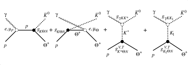
Figure 1: Feynman diagrams for $\Theta^{+}$ photoproduction on the proton $\gamma+p\longrightarrow{\bar{K}}^{0}+\Theta^{+}$.

The inclusion of hadronic form factors at hadronic vertices is performed by utilizing the Haberzettl prescription Haberzettl:1998eq . The form factors in this calculation are taken as

$$F_{i}(q^{2}) = \frac{\Lambda^{4}}{\Lambda^{4}+(q^{2}-m_{i}^{2})^{2}}$$ (7)

with $q^{2}=s,u,t$, and $i=p,\Theta,{\bar{K}}$, while $\Lambda$ the corresponding cut-off. The form factor for non-gauge-invariant terms ${\widetilde{F}}(s,u,t)$ in Eq. (3) is extra constructed in order to satisfy crossing symmetry and to avoid a pole in the amplitude Davidson:2001rk .

The coupling constant $g_{K\Theta N}$ is calculated from the decay width of the $\Theta^{+}\to K^{+}n$ by using

$$\Gamma = \frac{g^{2}_{K^{-}\Theta^{+}n}}{4\pi}\,\frac{E_{n}-m_{n}}{m_{\Theta}}\,p~{},$$ (8)

with

$$p=\frac{[\{m_{\Theta}^{2}-(m_{K}+m_{n})^{2}\}\{m_{\Theta}^{2}-(m_{n}-m_{K})^{2}\}]^{1/2}}{2m_{\Theta}}$$ (9)

The precise measurement of the decay width is still lacking due to the experimental resolution. The reported width is in the range of 6–25 MeV leps ; saphir ; clas ; diana ; hermes ; svd ; nusinov . Theoretical analyses of $K^{+}N$ data result in $\Gamma\leq 1$ MeV theor_anal , whereas the Particle Data Group pdg2004 ; cahn announces $\Gamma=0.9\pm 0.3$ MeV. Based on this information, we decided to use a width of 1 MeV in our calculation. We find that the isobar model becomes no longer sensitive to the value of $g_{K\Theta N}$ coupling constant, once we have included the $K^{*}$ and $K_{1}$ exchanges. Explicitly, we use

$$\frac{g_{K\Theta N}}{\sqrt{4\pi}} = 0.39~{}.$$ (10)

The magnetic moment of $\Theta^{+}$ is also not well known. A recent chiral soliton calculation kim2003 yields a value of $\mu_{\Theta}=0.82~{}\mu_{N}$, from which we obtain $\kappa_{\Theta}=0.35$. As in the case of $g_{K\Theta N}$ coupling constant, our calculation is also not sensitive to the numerical value of $\Theta^{+}$ magnetic moment, so that we feel it is save to use the above value. Note that the Regge model does not depend on this coupling constant as well as the $\Theta^{+}$ magnetic moment.

The transition moment is related to the radiative decay width by

$$\Gamma_{K^{*}\to K\gamma}=\frac{\alpha}{24}\left(\frac{g_{K^{*}K\gamma}}{M}\right)^{2}\,\left[m_{K^{*}}\left(1-\frac{m_{K}^{2}}{m_{K^{*}}^{2}}\right)\right]^{3}.$$ (11)

The decay width for $K^{*0}(892)$ is well known, i.e. pdg2004

$$\Gamma_{K^{*0}\rightarrow K^{0}\gamma} = 116\pm 10~{}~{}{\rm keV}~{}.$$ (12)

Thus, we obtain $g_{K^{*0}K^{0}\gamma}=-1.27$, where we have used the quark model prediction of Singer and Miller singer in order to constrain the relative sign.

The coupling constants $g^{V}_{K^{*}\Theta N}$ and $g^{T}_{K^{*}\Theta N}$ are also not well known. Therefore, we follow Refs. yu&ji2004 ; liu&ko2004 , i.e., using $g^{V}_{K^{*}\Theta N}=1.32$ and neglecting $g^{T}_{K^{*}\Theta N}$ due to lack of information on this coupling. By combining the electromagnetic and hadronic coupling constants we obtain

$$\frac{G^{V}_{K^{*}\Theta N}}{4\pi} = 8.72\times 10^{-2}~{}.$$ (13)

Most previous calculations excluded the $K_{1}$ exchange, mainly due to the lack of information on the corresponding coupling constants. Reference yu&ji2004 used the vector dominance relation $g_{K_{1}K\gamma}=eg_{K_{1}K\rho}/f_{\rho}$ to determine the electromagnetic coupling $g_{K_{1}K\gamma}$, where $f^{2}_{\rho}/4\pi=2.9$ and $g_{K_{1}K\rho}=12$ is taken from the effective Lagrangian calculation of Ref. haglin94 . As in the case of $K^{*}$, the $K_{1}$ hadronic tensor coupling will be neglected in this calculation due to the same reason. Following Ref. yu&ji2004 , the $K_{1}$ axial vector coupling $g^{V}_{K_{1}\Theta N}$ is estimated from an isobar model for $K^{+}\Lambda$ photoproduction by using the extracted $G^{V}_{K^{*}\Lambda N}/G^{V}_{K_{1}\Lambda N}$ ratio. However, instead of using the result of WJC model wjc we will exploit the extracted ratio found in Ref. mart2000 . There are two models given in Ref. mart2000 , i.e., models with and without the missing resonance $D_{13}(1895)$, which give a ratio of $-0.24$ and $-8.25$, respectively. Incidentally, Ref. wjc gives a ratio of $-8.26$, i.e., similar to the model without missing resonance. In our calculation we will use this ratio and excluding the result from the model with missing resonance, since the later leads to a divergence contribution to the GDH sum rule, as will be described later. In summary, in our calculation we use

$$\frac{G^{V}_{K_{1}\Theta N}}{4\pi} = -7.64\times 10^{-3}~{}.$$ (14)

The cross section can be easily calculated from the functions $A_{i}$ given by Eqs. (2)–(5) deo .

For the Regge model one should only use the last two diagrams in Fig. 1. Hence, the result from Regge model will not depend on the value of $g_{K\Theta N}$ and $\Theta^{+}$ magnetic moment. The procedure is adopted from Ref. guidal97 , i.e., by replacing the Feynman propagator with the Regge propagator

$$P_{\rm Regge} = \frac{s^{\alpha_{K^{i}}(t)-1}}{\sin[\pi\alpha_{K^{i}}(t)]}~{}e^{-i\pi\alpha_{K^{i}}(t)}~{}\frac{\pi\alpha_{K^{i}}^{\prime}}{\Gamma[\pi\alpha_{K^{i}}(t)]}~{},$$ (15)

where $K^{i}$ refers to $K^{*}$ and $K_{1}$, and $\alpha_{K^{i}}(t)=\alpha_{0}+\alpha^{\prime}\,t$ denotes the corresponding trajectory guidal97 . We note that Ref. guidal97 used form factors for extending the model to larger momentum transfer (“hard” process region). In our calculation we do not use these form factors, since the corresponding cross sections at this region are already quite small and, therefore, will not strongly influence the result of our calculation. We also note that systematic analyses of experimental data on $\rho$, $\omega$, and $J/\Psi$ photoproductions explicitely require hadronic form factors regge_rho .

In both models, however, we can also calculate the spin dependent total cross sections

$$\sigma_{\rm T}=\frac{\sigma_{3/2}+\sigma_{1/2}}{2}~{}~{}~{}\textrm{and}~{}~{}\sigma_{\rm TT^{\prime}}=\frac{\sigma_{3/2}-\sigma_{1/2}}{2},$$ (16)

where the latter is of special interest since it can be related to the proton anomalous magnetic moment $\kappa_{p}$ using the GDH sum rule

$$-\frac{2\pi^{2}\alpha\kappa_{p}^{2}}{m_{p}^{2}}=\int_{0}^{\infty}\frac{d\nu}{\nu}[\sigma_{1/2}(\nu)-\sigma_{3/2}(\nu)]~{}\equiv~{}I_{\rm GDH},$$ (17)

with $\nu=E_{\gamma}^{\rm lab}$ and $\sigma_{1/2}$ ($\sigma_{3/2}$) represents the cross section for possible proton and photon spin combinations with a total spin of $1/2$ ($3/2$). Thus, we can calculate contribution of the $\Theta^{+}$ photoproduction to the GDH integral $I_{\rm GDH}$ defined by Eq. (17). Note that in deriving Eq. (17) it has been assumed that the scattering amplitude goes to zero in the limit of $|\nu|\rightarrow\infty$ sbass .

Figure 2: Total cross sections $\sigma_{\rm T}$ and $-\sigma_{\rm TT^{\prime}}$ of the isobar and Regge models. In isobar model variation of the total cross section for different hadronic form factor cut-offs is shown.

The result of our calculation is depicted in Fig. 2, where we compare the total cross section obtained from isobar model with different hadronic cut-offs and that from the Regge model. Obviously, the hadronic cut-off strongly controls the magnitude of the cross section in the isobar model. By varying $\Lambda$ from 0.6 to 1.2, both total cross sections increase by two orders of magnitude, whereas their shapes remain stable and tend to saturate at high energies. In the Regge model, both $\sigma_{\rm T}$ and $-\sigma_{\rm TT^{\prime}}$ steeply rise to maximum at $W$ around 2.2 GeV and monotonically decrease after that. Regge cross sections are clearly more convergent than isobar ones. From threshold up to $W=3$ GeV, the cross section magnitude of the Regge model falls between the results obtained from isobar model with $\Lambda=0.6$ and 0.8 GeV. Starting from $W=3$ GeV, the magnitude becomes smaller than the result from isobar model with $\Lambda=0.6$ GeV. Thus, future calculation should consider the hadronic cut-off in the range of 0.6 and 0.8 GeV.

Figure 3: Contribution of the $\Theta^{+}$ photoproduction to the GDH integral of the proton for isobar (with different hadronic form factor cut-offs) and Regge models.

Contribution from the pentaquark photoproduction to the GDH integral is shown in Fig. 3, where we compare the result from isobar and Regge models as in Fig. 2. Clearly, the contribution is positive and small [note that direct calculation of the l.h.s. of Eq. (17) gives $-205~{}\mu$b]. Nevertheless, the positive contribution to $I_{\rm GDH}$ invites an interesting discussion if we consider the current knowledge of the GDH individual contribution on the proton. By summing up contributions from $\pi$, $\eta$, $\pi\pi$, and $K$ photoproduction, including contribution from the higher energy part, Ref. drechsel found an $I_{\rm GDH}=-202~{}\mu$b. Recent calculation on vector meson ($\omega$, $\rho^{0}$, and $\rho^{+}$) contributions qzhao indicates that their total contribution is also small ($+0.26~{}\mu$b). From this point of view, negative (or positive but small) contribution is more preferred. In other words, prediction from Regge model is more desired rather than those of isobar model with $\Lambda\geq 0.8$ GeV.

As previously mentioned, the isobar model which includes the missing resonance mart2000 yields a ratio of $G^{V}_{K^{*}\Lambda N}/G^{V}_{K_{1}\Lambda N}=-0.24$. Using this ratio, we found that the predicted $-\sigma_{\rm TT^{\prime}}$ flips to negative values at $W$ around 3 GeV and starts to diverge from that point. This behavior merely emphasizes that certain mechanism (resonance exchanges) is missing in the process. Therefore, in our calculation we do not use this ratio.

Figure 4: Differential cross section for $\Theta^{+}$ photoproduction on the proton as functions of $\cos\theta$ and $W$ from isobar model obtained with $\Lambda=1$ GeV. The same pattern, but with the magnitude 20 times smaller, would be obtained if one used $\Lambda=0.6$ GeV.

Recent isobar calculation for $K^{+}\Lambda$ photoproduction janssen claimed that a soft hadronic form factor (small $\Lambda$) is not desired by the field theory. A harder form factor is achieved by including some $u$-channel resonances in the model. However, the authors do not build an explicit relation of this statement with the field theory. At tree level the extracted coupling constants are assumed to effectively absorb some important ingredients in the process, such as rescattering terms and higher order corrections, which are clearly beyond the scope of an isobar model. Therefore, the constants cannot be separated from the form factors. Together, they define the effective coupling constants. Hence, it is hard to say that at tree level calculation an isobar model should simultaneously produce SU(3) coupling constants and large cut-offs, i.e., weak suppression on the divergent Born terms. A careful examination on the $u$-channel resonance coupling constants reveals the fact that the corresponding error bars are relatively large, which indicates that the inclusion of these resonances is trivial petr .

Figure 5: Differential cross section for $\Theta^{+}$ photoproduction on the proton as functions of $\cos\theta$ and $W$ from Regge model.

The predicted differential cross sections are shown in Figs. 4 and 5. The result shown in Fig. 4 is obtained by using $\Lambda=1$ GeV. By varying the $\Lambda$ value, only the magnitude of the cross section changes, whereas its shape with respect to $W$ and $\cos\theta$ remains stable. Thus, the difference between isobar and Regge models is quite apparent in these figures. The isobar model limits measurements only at $0\leq\cos\theta\leq 0.5$, while Regge model allows for a complete angular distribution of differential cross section at energies between threshold and 2.5 GeV. At smaller $\cos\theta$ the cross section increases with $W$ and becomes constant for $W>3.5$ GeV, in contrast to the prediction from isobar model, which sharply increases as a function of $W$. Future experimental measurements at JLab, SPRING-8, or ELSA will certainly be able to settle this problem.

In conclusion we have simultaneously investigated $\Theta^{+}$ photoproduction by using isobar and Regge models. We found that a comparable result is achieved if we use a hadronic cut-off between 0.6–0.8 GeV. This result indicates that previous calculations which used a harder hadronic form factor are probably overestimates. By calculating the contribution to the GDH integral we found that Regge model and isobar model with $\Lambda\leq 0.6$ GeV are favorable.

This work has been supported in part by the QUE (Quality for Undergraduate Education) project.

References

- (1) T. Nakano et al., Phys. Rev. Lett. 91, 012002 (2003).
- (2) J. Barth et al., Phys. Lett. B 572, 127 (2003).
- (3) S. Stepanyan et al., Phys. Rev. Lett. 91, 252001 (2003); V. Kubarovsky et al., Phys. Rev. Lett. 92, 032001 (2004).
- (4) V. V. Barmin et al., Phys. Atom Nucl. 66, 1715 (2003).
- (5) A. Airapetian et al., Phys. Lett. B 585, 213 (2004).
- (6) D. Diakonov, V. Petrov, and M. Polyakov, Z. Phys. A 359, 305 (1997).
- (7) M. Karliner and H. J. Lipkin, Phys. Lett. B 597, 309 (2004)
- (8) A. I. Titov, A. Hosaka, S. Date and Y. Ohashi, Phys. Rev. C 70, 042202(R) (2004).
- (9) Y. Oh, H. C. Kim, and S. H. Lee, Phys. Rev. D 69 014009 (2004).
- (10) S. I. Nam, A. Hosaka, and H.-Ch. Kim, Phys. Lett. B 579, 43 (2004).
- (11) Y. R. Liu, P. Z. Huang, W. Z. Deng, X. L. Chen and S. L. Zhu, Phys. Rev. C 69, 035205 (2004)
- (12) W. W. Li et al., High Energy Phys. Nucl. Phys. 28, 918 (2004).
- (13) P. Ko, J. Lee, T. Lee and J. h. Park, hep-ph/0312147.
- (14) W. Liu, C. M. Ko, and V. Kubarovsky, Phys. Rev. C 69, 025202 (2004).
- (15) B. G. Yu, T. K. Choi, and C.-R. Ji, Phys. Rev. C 70, 045205 (2004).
- (16) Q. Zhao, J. S. Al-Khalili, and C. Bennhold, Phys. Rev. C 65, 032201(R) (2002).
- (17) T. Mart and C. Bennhold, Phys. Rev. C 61, 012201(R) (2000); Kaon-Maid, http://www.kph.uni-mainz. de/MAID/kaon/kaonmaid.html.
- (18) M. Guidal, J. M. Laget, and M. Vanderhaeghen, Nucl. Phys. A627, 645 (1997).
- (19) T. Mart and T. Wijaya, Acta Phys. Polon. B 34, 2651 (2003).
- (20) W. T. Chiang, S. N. Yang, L. Tiator, M. Vanderhaeghen and D. Drechsel, Phys. Rev. C 68, 045202 (2003).
- (21) D. Drechsel, S. S. Kamalov, and L. Tiator, Phys. Rev. D 63, 114010 (2001).
- (22) F. X. Lee, T. Mart, C. Bennhold and L. E. Wright, Nucl. Phys. A695, 237 (2001).
- (23) H. Haberzettl, C. Bennhold, T. Mart, and T. Feuster, Phys. Rev. C 58, R40 (1998).
- (24) R. M. Davidson and R. Workman, Phys. Rev. C 63, 025210 (2001).
- (25) A. Aleev et al., hep-ex/0401024
- (26) S. Nussinov, hep-ph/0307357 (2003).
- (27) R. A. Arndt, I. I. Strakovsky, and R. L. Workman, nucl-th/0311030 (2003); W. R. Gibbs, Phys. Rev. C 70, 045208 (2004); A. Sibirtsev, J. Haidenbauer, S. Krewald, Ulf-G. Meissner, Phys. Lett. B 599, 230 (2004).
- (28) Particle Data Group: S. Eidelman et al., Phys. Lett. B 592, 1 (2004).
- (29) R. N. Cahn and G. H. Trilling, Phys. Rev. D 69, 011501 (2004).
- (30) Hyun-Chul Kim, Phys. Lett. B 585, 99 (2004).
- (31) P. Singer and G. A. Miller, Phys. Rev. D 33, 141 (1986).
- (32) K. Haglin, Phys. Rev. C 50, 1688 (1994).
- (33) R. A. Williams, C.-R. Ji, and S. R. Cotanch, Phys. Rev. C 46, 1617 (1992).
- (34) B. B. Deo and A. K. Bisoi, Phys. Rev. D 9, 288 (1974); G. Knöchlein, D. Drechsel, and L. Tiator, Z. Phys. A 352, 327 (1995).
- (35) A. Donnachie and P. V. Landshoff, Phys. Lett. B 478, 146 (2000); A. Sibirtsev, K. Tsushima and S. Krewald, Phys. Rev. C 67, 055201 (2003); A. Sibirtsev, S. Krewald and A. W. Thomas, J. Phys. G 30, 1427 (2004).
- (36) S. D. Bass, Z. Phys. A 355, 77 (1996).
- (37) S. Janssen, J. Ryckebusch, D. Debruyne, and T. Van Cauteren, Phys. Rev. C. 65, 015201 (2002).
- (38) P. Bydzovsky, private communication.