Density Functional Theory: Methods and Problems

Abstract

The application of density functional theory to nuclear structure is discussed, highlighting the current status of the effective action approach using effective field theory, and outlining future challenges.

1 Introduction

The similarities between self-consistent mean-field approaches to nuclear structure, such as Skyrme Hartree–Fock [1, 2], and Kohn-Sham density functional theory (DFT), which is widely applied to Coulomb many-body problems [3], are frequently noted. To go beyond the simple surface comparisons, however, there are many questions to address about applying DFT methods to nuclear structure and potential problems or challenges one will confront in trying to connect the two. For example,

• How is Kohn-Sham DFT more than a mean-field calculation? Where are the approximations? How do we include long-range effects in a Skyrme-like formalism?

• What can you calculate in a DFT approach? Excited states? What about single-particle properties?

• How does pairing work in DFT? Are higher-order contributions important?

• How do we deal with broken symmetries (translation, rotation, …)?

• Can we connect quantitatively to the free NN interaction? What about to chiral effective field theory (EFT) and/or low-momentum interactions?

In this talk, we discuss how to make the nuclear connection to DFT systematically, by building a framework for addressing these questions. The idea is to use effective actions of composite operators to develop DFT [4], with the Kohn-Sham orbitals arising through the inversion method used to effect the Legendre transformation to the effective action [5, 6]. The inversion method requires a hierarchy of approximations; here this is provided by an effective field theory expansion, which uses power counting to tell us what diagrams to include at each order [7]. Ultimately, we seek nuclear energy functionals similar to conventional “phenomenological” approaches but model independent, with error estimates, and derivable from microscopic EFT approaches.

2 Effective Action Approach to EFT-Based Kohn-Sham DFT

The dominant use of density functional theory (DFT) is in the description of interacting point electrons in the static potential of atomic nuclei. Applications include calculations of atoms, molecules, crystals, and surfaces [3]. Discussions of DFT typically start with a proof by contradiction of the existence of the Hohenberg-Kohn (HK) energy functional

$$E_{v}[\rho]=F_{\rm HK}[\rho]+\int\!d^{3}x\,v({\bf x})\rho({\bf x})\ ,$$ (1)

which is minimized at the exact ground-state energy by the exact ground-state density, and where $F_{\rm HK}[\rho]$ is universal. The Kohn-Sham procedure further posits a non-interacting system with the same density as the fully interacting system [3]. This leads to constructing $E_{v}$ using single-particle orbitals in a local potential $v_{\rm KS}({\bf x})$,

$$[-\bm{\nabla}^{2}/2m+v_{\rm KS}({\bf x})]\phi_{i}={\varepsilon_{i}}\phi_{i}\ \Longrightarrow\ \rho({\bf x})=\sum_{i=1}^{N}|\phi_{i}({\bf x})|^{2}\ ,$$ (2)

which is determined self-consistently from $E_{v}[\rho]$. The relative simplicity of solving Eq. (2) for large finite systems is apparent while the entire approach is a win if there are reasonable approximations to $F_{\rm HK}[\rho]$, such as the local density approximation (LDA).

We rely on a thermodynamic derivation of DFT, which uses the effective action formalism [8] to construct energy density functionals [4, 5]. The basic plan is to consider the partition function ${\cal Z}$ for the (finite) system of interest in the presence of external sources coupled to various quantities of interest (such as the density). We derive energy functionals of these quantities by Legendre transformations with respect to the sources. These sources probe, in a variational sense, configurations near the ground state.

To derive conventional density functional theory, we consider an external source $J(x)$ coupled to the density operator $\widehat{\rho}(x)\equiv\psi^{\dagger}(x)\psi(x)$ in the partition function

$${\cal Z}[J]=e^{-W[J]}\sim{\rm Tr\,}e^{-\beta(\widehat{H}+J\,\widehat{\rho})}\sim\int\!{\cal D}[\psi^{\dagger}]{\cal D}[\psi]\,e^{-\int[{\cal L}+J\,\psi^{\dagger}\psi]}\ ,$$ (3)

for which we will construct a path integral representation with Lagrangian ${\cal L}$ [8]. (Note: for convenience, we will take the inverse temperature $\beta$ and the volume $V$ equal to unity in the sequel.) The (time-dependent) density $\rho(x)$ in the presence of $J(x)$ is

$$\rho(x)\equiv\langle\widehat{\rho}(x)\rangle_{J}=\frac{\delta W[J]}{\delta J(x)}\ ,$$ (4)

which we invert to find $J[\rho]$ and then Legendre transform from $J$ to $\rho$:

$$\Gamma[\rho]=-W[J]+\int\!J\,\rho\quad\mbox{with}\quad J(x)=\frac{\delta\Gamma[\rho]}{\delta\rho(x)}\longrightarrow\left.\frac{\delta\Gamma[\rho]}{\delta\rho(x)}\right|_{\rho_{\rm gs}({\bf x})}=0\ .$$ (5)

For static $\rho({\bf x})$, $\Gamma[\rho]$ is proportional to the DFT energy functional $F_{\rm HK}$!

We still need a way to carry out the inversion; for this we rely on the inversion method of Fukuda et al. [4]. The idea is to expand the relevant quantities in a hierarchy,

$$W[J,\lambda] \!=\! W_{0}[J]+\lambda W_{1}[J]+\lambda^{2}W_{2}[J]+\cdots\ ,$$ (6)

$$J[\rho,\lambda] \!=\! J_{0}[\rho]+\lambda J_{1}[\rho]+\lambda^{2}J_{2}[\rho]+\cdots\ ,$$ (7)

$$\Gamma[\rho,\lambda] \!=\! \Gamma_{0}[\rho]+\lambda\Gamma_{1}[\rho]+\lambda^{2}\Gamma_{2}[\rho]+\cdots\ ,$$ (8)

treating $\rho$ as order unity, and match order by order in $\lambda$. Zeroth order is a noninteracting system with potential $J_{0}(x)$:

$$\Gamma_{0}[\rho]=-W_{0}[J_{0}]+\int\!d^{4}x\,J_{0}(x)\rho(x)\quad\Longrightarrow\quad\rho(x)=\frac{\delta W_{0}[J_{0}]}{\delta J_{0}(x)}\ .$$ (9)

Because $\rho$ appears only at zeroth order, it is given exactly from the non-interacting system according to Eq. (9). This is the Kohn-Sham system with the exact density! We diagonalize $W_{0}[J_{0}]$ by introducing Kohn-Sham orbitals as in Eq. (2); it is the sum of $\varepsilon_{i}$’s. Finally, we find $J_{0}$ for the ground state by completing a self-consistency loop:

$${J_{0}}\rightarrow W_{1}\rightarrow\Gamma_{1}\rightarrow J_{1}\rightarrow W_{2}\rightarrow\Gamma_{2}\rightarrow\cdots\Longrightarrow{J_{0}(x)=-\sum_{i>0}J_{i}(x)=\sum_{i>0}\frac{\delta\Gamma_{i}[\rho]}{\delta\rho(x)}}\ .$$ (10)

Note that even though solving for Kohn-Sham orbitals makes the approach look like mean field, the approximation to the energy and density is only in the truncation of Eq. (10) at some order. Further, by using time-dependent sources we can generalize RPA to time-dependent DFT, to calculate properties of collective excitations.

The hierarchy we have in mind is defined by EFT power counting. For example, the EFT for a dilute Fermi system with short-range interactions is defined by a general interaction as the sum of delta functions and their derivatives. In momentum space,

$$\langle{\bf k}|V_{\rm eft}|{\bf k^{\prime}}\rangle=C_{0}+\frac{1}{2}C_{2}({\bf k}^{2}+{\bf k^{\prime}}^{2})+C^{\prime}_{2}{\bf k\cdot k^{\prime}}+\cdots\ ,$$ (11)

which corresponds to ${\cal L}_{\rm eft}$ with general contact interactions (including $3+$ bodies):

$${\cal L}_{\rm eft} = \psi^{\dagger}\Bigl{[}i\frac{\partial}{\partial t}+\frac{\overrightarrow{\nabla}^{\,2}}{2M}\Bigr{]}\psi-\frac{C_{0}}{2}(\psi^{\dagger}\psi)^{2}+\frac{C_{2}}{16}\bigl{[}(\psi\psi)^{\dagger}(\psi\!\stackrel{{\scriptstyle\leftrightarrow}}{{\nabla}}\!{}^{2}\psi)+\mbox{ h.c.}\bigr{]}$$ (12)

$$\hbox{}+\frac{C_{2}^{\prime}}{8}(\psi\!\stackrel{{\scriptstyle\leftrightarrow}}{{\nabla}}\!\psi)^{\dagger}\cdot(\psi\!\stackrel{{\scriptstyle\leftrightarrow}}{{\nabla}}\!\psi)-\frac{D_{0}}{6}(\psi^{\dagger}\psi)^{3}+\ldots\ .$$

Dimensional analysis implies that $C_{2i}\sim\frac{\textstyle 4\pi}{\textstyle M}R^{2i+1}\,,D_{2i}\sim\frac{\textstyle 4\pi}{\textstyle M}R^{2i+4}$, where $R$ is the range of the interaction, which gives our hierarchy (e.g., if $k_{\scriptscriptstyle\rm F}R\ll 1$). This ${\cal L}_{\rm eft}$ will generate functionals like conventional Skyrme functionals (but with a different power counting).

The conventional diagrammatic expansion of the propagator takes the form

$\Longrightarrow$ 

with a non-local, state-dependent $\Sigma^{\ast}({\bf x},{\bf x}^{\prime};\omega)$. In contrast, in Kohn-Sham DFT we have a local $J_{0}({\bf x})$ to all orders (i.e., not just at the Hartree level):

which introduces new Feynman rules for the “inverse density-density correlator” (double line) corresponding to $[\delta\rho({\bf x})/\delta J_{0}({\bf y})]^{-1}$. These inverse correlators appear in the energy,

(13)

but in this case the last two diagrams precisely cancel, in complete analogy to the cancellation of anomalous diagrams according to Kohn, Luttinger, and Ward [8].

We can show how the full Green’s function $G$ is related to the Kohn-Sham Green’s function $G_{\rm ks}$ by adding a non-local source $\xi(x,x^{\prime})$ coupled to $\psi(x)\psi^{\dagger}(x^{\prime})$ [9]:

$$Z[J,\xi]=e^{-W[J,\xi]}=\int\!D\psi D\psi^{\dagger}\ e^{-\int\!d^{4}x\ [{\cal L}\,+\,J(x)\psi^{\dagger}(x)\psi(x)\,{+\,\int\!d^{4}x^{\prime}\,\psi(x)\xi(x,x^{\prime})\psi^{\dagger}(x^{\prime})}]}$$ (14)

The Green’s function follows as a functional derivative of $W$ with respect to $\xi$ at constant $J$, which is in turn equal to a functional derivative of $\Gamma$ with respect to $\xi$ at constant $\rho$. Since $\Gamma$ can be decomposed as $\Gamma_{0}$ from Eq. (9) plus everything else,

$$\Gamma[\rho,\xi]=\Gamma_{0}[\rho,\xi]+\Gamma_{\rm int}[\rho,\xi]\ ,$$ (15)

and $G_{\rm ks}$ is the full Green’s function for $\Gamma_{0}$, we can derive a Dyson-like equation:

$$G(x,x^{\prime})=\left.\frac{\delta W}{\delta\xi}\right|_{J}=\left.\frac{\delta\Gamma}{\delta\xi}\right|_{\rho}=G_{\rm ks}(x,x^{\prime})+G_{\rm ks}\Bigl{[}\frac{\delta\Gamma_{\rm int}}{\delta G_{\rm ks}}-\frac{\delta\Gamma_{\rm int}}{\delta\rho}\Bigr{]}G_{\rm ks}\ ,$$ (16)

represented diagrammatically as:

(17)

We find a simple diagrammatic proof that the density from the exact Green’s function (by taking a trace) equals the density of the non-interacting Kohn-Sham propagator:

(18)

but other observables quantities of interest, such as single-particle properties, will generally differ and will need to be calculated using Eq. (17).

To study further how well single-particle properties are reproduced, we include the kinetic energy density $\tau(x)\equiv\langle\bm{\nabla}\psi^{\dagger}\cdot\bm{\nabla}\psi\rangle$ in the DFT formulation for fermions in a trap. The meta-GGA DFT for the Coulomb problem uses $\tau$ as an ingredient in the energy functionals, but applies a semi-classical expansion in terms of the density [3]. The result is a Kohn-Sham equation with a local potential only. In contrast, in Skyrme Hartree-Fock (SHF), $\rho$ and $\tau$ are treated as independent ($N=Z$ nuclei here [1]):

$$E_{\rm SHF}[\rho,\tau,{\bf J}] = \int\!d^{3}x\,\biggl{\{}{1\over 2M}\tau+{3\over 8}t_{0}\rho^{2}+{1\over 16}t_{3}\rho^{2+\alpha}+{1\over 16}(3t_{1}+5t_{2})\rho\tau$$ (19)

$$\hbox{}+{1\over 64}(9t_{1}-5t_{2})(\bm{\nabla}\rho)^{2}-{3\over 4}W_{0}\rho\bm{\nabla}\cdot{\bf J}+{1\over 32}(t_{1}-t_{2}){\bf J}^{2}\biggr{\}}\ ,$$

(${\bf J}$ is a spin-orbit density) and the orbital equations now have effective mass $M^{*}({\bf x})$.

To generate the analogous functional in DFT/EFT, add to the Lagrangian $\eta({\bf x})\,\bm{\nabla}\psi^{\dagger}\bm{\nabla}\psi$ and Legendre transform to an effective action of $\rho$ and $\tau$:

$$\Gamma[\rho,\tau]=W[J,\eta]-\int\!J(x)\rho(x)-\int\!\eta(x)\tau(x)\ .$$ (20)

The inversion method results in two Kohn-Sham potentials,

$$J_{0}({\bf x})=\frac{\delta\Gamma_{\rm int}[\rho,\tau]}{\delta\rho({\bf x})}\quad\mbox{and}\quad\eta_{0}({\bf x})=\frac{\delta\Gamma_{\rm int}[\rho,\tau]}{\delta\tau({\bf x})}\ .$$ (21)

We diagonalize the quadratic part of the Lagrangian in $W_{0}$,

$$\int\!d^{4}x\ \psi^{\dagger}\biggl{[}i\partial_{t}+\frac{\bm{\nabla}^{\,2}}{2M}-v({\bf x})+J_{0}({\bf x})-\bm{\nabla}\cdot\eta_{0}({\bf x})\bm{\nabla}\biggr{]}\psi$$ (22)

and the Kohn-Sham equation becomes [with $v_{\rm KS}\equiv v({\bf x})-J_{0}({\bf x})$]

$$\bigl{[}-\bm{\nabla}{\frac{1}{M^{*}({\bf{x}})}}\bm{\nabla}+v_{\rm KS}({\bf x})\bigr{]}\,\psi_{\alpha}=\epsilon_{\alpha}\psi_{\alpha}$$ (23)

with an effective mass $1/2M^{*}({\bf x})\equiv 1/2M-\eta_{0}({\bf x})$, just like in Skyrme HF [9].

To highlight the differences between an energy functional of $\rho$ alone and one of $\rho$ and $\tau$, we focus on the Hartree-Fock contributions from vertices with derivatives:

$${\cal L}_{\rm eft}=\ldots+\frac{C_{2}}{16}\bigl{[}(\psi\psi)^{\dagger}(\psi\!\stackrel{{\scriptstyle\leftrightarrow}}{{\nabla}}\!{}^{2}\psi)+\mbox{ h.c.}\bigr{]}+\frac{C_{2}^{\prime}}{8}(\psi\!\stackrel{{\scriptstyle\leftrightarrow}}{{\nabla}}\!\psi)^{\dagger}\cdot(\psi\!\stackrel{{\scriptstyle\leftrightarrow}}{{\nabla}}\!\psi)+\ldots\ .$$ (24)

The corresponding part of the energy density with spin degeneracy $\nu=2$ for Kohn-Sham LDA is [6]

$${\cal E}_{\rm int}[\rho]=\ldots+\frac{C_{2}}{8}\Bigl{[}\frac{3}{5}\left(\frac{6\pi^{2}}{\nu}\right)^{2/3}\rho^{8/3}\Bigr{]}+\frac{3C_{2}^{\prime}}{8}\Bigl{[}\frac{3}{5}\left(\frac{6\pi^{2}}{\nu}\right)^{2/3}\rho^{8/3}\Bigr{]}+\ldots$$ (25)

and with $\tau$ is [10]

$${\cal E}_{\rm int}[\rho,\tau]=\ldots+\frac{C_{2}}{8}\bigl{[}\rho\tau+\frac{3}{4}(\bm{\nabla}\rho)^{2}\bigr{]}+\frac{3C_{2}^{\prime}}{8}\bigl{[}\rho\tau-\frac{1}{4}(\bm{\nabla}\rho)^{2}\bigr{]}+\ldots\ .$$ (26)

The $\rho\tau$ functional with $\nu=4$ takes the same form as the Skyrme functional with $C_{i}\rightarrow t_{i}$. (To get the spin-orbit part, one should couple a source to the spin-orbit density.)

   

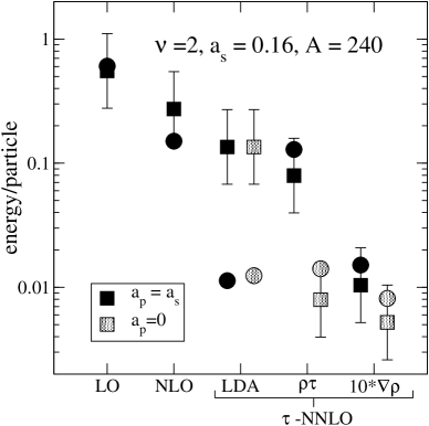
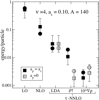
Figure 1: Contributions to the energy for two systems of trapped fermions [10].

First, we note that power counting estimates work for all terms in the $\rho\tau$ energy functional, as shown for two examples in Fig. 1 [the “$\rho\tau$” and “$\nabla\rho$” contributions are from Eq. (26)]. The squares with error bars are estimated contributions to the energy per particle from terms in the energy functional at each order. The error bars indicate a “natural” range of coefficients between 1/2 and 2. The circles are the actual values. The hierarchy as well as the accuracy of the predictions is evident [10].

$a_{p}=a_{s}$ $E/A$ $\sqrt{\langle r^{2}\rangle}$ $\rho$ 7.66 2.87 $\rho\tau$ 7.65 2.87 $a_{p}=2a_{s}$ $E/A$ $\sqrt{\langle r^{2}\rangle}$ $\rho$ 8.33 3.10 $\rho\tau$ 8.30 3.09      

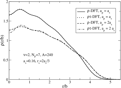
Figure 2: Results for the $\rho$ and $\rho\tau$ functionals for representative cases [10].

We also note from these figures that the contributions that are new to the $\rho\tau$ functional are very small. Thus, we are not surprised to find that predicted bulk observables are very similar (see Fig. 2). The total binding energy and density are what Kohn-Sham is supposed to get right. What about the single-particle spectrum? The effective mass is unity in the $\rho$ case and, as seen in Fig. 3(a), is reduced significantly in the $\rho\tau$ case (the central values roughly cover the range in typical Skyrme interactions). The different effective mass is reflected in the single-particle spectra in Fig. 3(b), which can be understood qualitatively from the spectra calculated in a uniform system,

$$\varepsilon_{\bf k}^{\rho}-\varepsilon_{\bf k}^{\rho\tau}=\frac{\pi}{\nu}[(\nu-1)a_{s}^{2}r_{s}+2(\nu+1)a_{p}^{3}]\,\frac{k_{F}^{2}-{\bf k}^{2}}{2M}\rho\ .$$ (27)

Even though the density and energy are the same, the spectra are not. However, the $\rho\tau$ result is closer to that of the full Green’s function, as can be shown from Eq. (17) [10].

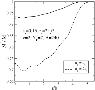
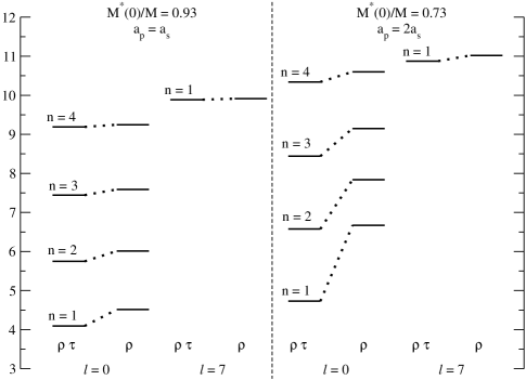
Figure 3: a) Effective mass and b) single-particle spectra for representative cases [10].

An important ingredient of energy functionals for nuclei is pairing, which requires another generalization of Kohn-Sham DFT. To do so, we introduce an external source $j$ coupled to the pair density, to break the $U(1)$ phase symmetry associated with fermion number. The generating functional now becomes

$$Z[J,\/j]=e^{-W[J,\/j]}=\int\!D(\psi^{\dagger}\psi)\ e^{-\int\!d^{4}x\ [{\cal L}\,+\,J(x)\psi_{\alpha}^{\dagger}\psi_{\alpha}\,+\,j(x)(\psi^{\dagger}_{\uparrow}\psi^{\dagger}_{\downarrow}+\psi_{\downarrow}\psi_{\uparrow})]}\ ,$$ (28)

and the fermion and pair densities $\rho,\phi$ are found by functional derivatives with respect to $J,j$:

$$\rho(x) \equiv \langle\psi^{\dagger}(x)\psi(x)\rangle_{J,j}=\left.\frac{\delta W[J,j]}{\delta J(x)}\right|_{j}\ ,$$ (29)

$$\phi(x) \equiv \langle\psi^{\dagger}_{\uparrow}(x)\psi^{\dagger}_{\downarrow}(x)+\psi_{\downarrow}(x)\psi_{\uparrow}(x)\rangle_{J,j}=\left.\frac{\delta W[J,j]}{\delta j(x)}\right|_{J}\ .$$ (30)

The effective action $\Gamma[\rho,\phi]$ follows yet again by functional Legendre transformation:

$$\Gamma[\rho,\phi]=W[J,j]-\int\!d^{4}x\,J(x)\rho(x)-\int\!d^{4}x\,j(x)\phi(x)\ ,$$ (31)

and is proportional to the ground-state energy functional. The sources in turn are given by functionals derivatives with respect to $\rho$ and $\phi$, which are therefore determined in the ground state (where the sources are zero) by stationarity:

$$\left.\frac{\delta\Gamma[\rho,\phi]}{\delta\rho({\bf x})}\right|_{{\rho=\rho_{\rm gs},\phi=\phi_{\rm gs}}}=\left.\frac{\delta\Gamma[\rho,\phi]}{\delta\phi({\bf x})}\right|_{{\rho=\rho_{\rm gs},\phi=\phi_{\rm gs}}}=0\ .$$ (32)

This is Hohenberg-Kohn DFT extended to pairing!

Inversion is again carried out by order-by-order matching in an EFT expansion. Zeroth order is the Kohn-Sham system with potentials $J_{0}({\bf x})$ and $j_{0}({\bf x})$, which yields the exact densities $\rho({\bf x})$ and $\phi({\bf x})$. We introduce single-particle orbitals and solve

$$\left(\begin{array}[]{cc}h_{0}({\bf x})-\mu_{0}&j_{0}({\bf x})\\ j_{0}({\bf x})&-h_{0}({\bf x})+\mu_{0}\end{array}\right)\left(\begin{array}[]{c}u_{i}({\bf x})\\ v_{i}({\bf x})\end{array}\right)=E_{i}\left(\begin{array}[]{c}u_{i}({\bf x})\\ v_{i}({\bf x})\end{array}\right)$$ (33)

where $u_{i},v_{i}$ satisfy conventional orthonormality relations [1, 2] and

$$h_{0}({\bf x})\equiv-\frac{\bm{\nabla}^{2}}{2M}+v({\bf x})-J_{0}({\bf x})\ .$$ (34)

Thus it looks like conventional Hartree-Fock-Bogoliubov (HFB)!

The diagrammatic expansion is the same as without pairing, but now uses Nambu-Gorkov matrix Green’s functions. The Kohn-Sham self-consistency procedure is the same as in Skyrme or RMF with pairing [1, 2]. In terms of the orbitals, the fermion density is given by

$$\rho({\bf x})=2\sum_{i}\,|v_{i}({\bf x})|^{2}\ ,$$ (35)

and the (bare, unrenormalized) pair density is

$$\phi_{\rm bare}({\bf x})=\sum_{i}\,[u_{i}^{*}({\bf x})v_{i}({\bf x})+u_{i}({\bf x})v_{i}^{*}({\bf x})]=2\sum_{i}u_{i}({\bf x})v_{i}({\bf x})\ .$$ (36)

The chemical potential $\mu_{0}$ is fixed by $\int\!\rho({\bf x})=A$ and diagrams for $\Gamma[\rho,\phi]=-E[\rho,\phi]$ yields Kohn-Sham potentials

$$J_{0}({\bf x})\Bigr{|}_{\rho=\rho_{\rm gs}}=\left.\frac{\delta{\Gamma}_{\rm int}[\rho,\phi]}{\delta\rho({\bf x})}\right|_{\rho=\rho_{\rm gs}}\ \mbox{and}\quad j_{0}({\bf x})\Bigr{|}_{\phi=\phi_{\rm gs}}=\left.\frac{\delta{\Gamma}_{\rm int}[\rho,\phi]}{\delta\phi({\bf x})}\right|_{\phi=\phi_{\rm gs}}\ .$$ (37)

The pair density is divergent and requires renormalization. This problem is solved for a uniform system in Ref. [11] by introducing a counterterm proportional to $j^{2}$. In this uniform limit, $\phi$ is ultimately defined with a subtraction:

$$\phi=\int^{k_{c}}\!\frac{d^{3}k}{(2\pi)^{3}}\,j_{0}\left(\frac{1}{\sqrt{(\epsilon_{k}^{0}-\mu_{0})^{2}+j_{0}^{2}}}-\frac{1}{\epsilon_{k}^{0}}\right)\stackrel{{\scriptstyle k_{c}\rightarrow\infty}}{{\longrightarrow}}\mbox{finite}\ ,$$ (38)

which can be applied in a local density approximation (i.e., Thomas-Fermi),

$$\phi({\bf x})=2\sum_{i}^{E_{c}}u_{i}({\bf x})v_{i}({\bf x})-j_{0}({\bf x})\frac{Mk_{c}({\bf x})}{2\pi^{2}}\quad\mbox{with}\quad E_{c}=\frac{k_{c}^{2}({\bf x})}{2M}+v_{\rm KS}({\bf x})-\mu\ .$$ (39)

However, convergence is very slow as the energy cutoff $E_{c}$ is increased, which is a practical problem for implementation in nuclei. Bulgac and Yu have shown how one can make different subtractions and greatly improve the convergence [12]. For example, defining $\phi$ instead through

$$\phi=\int^{k_{c}}\!\frac{d^{3}k}{(2\pi)^{3}}\,j_{0}\left(\frac{1}{\sqrt{(\epsilon_{k}^{0}-\mu_{0})^{2}+j_{0}^{2}}}-\frac{{\cal P}}{\epsilon_{k}^{0}-\mu_{0}}\right)\stackrel{{\scriptstyle k_{c}\rightarrow\infty}}{{\longrightarrow}}\mbox{finite}$$ (40)

leads to much faster convergence, as seen here for the uniform system:

Bulgac has found even faster convergence with other subtractions.

A question to be investigated is the role of higher-order contributions. In the weak-coupling limit, the pairing gap in a dilute Fermi gas with two spin states is reduced approximately fifty percent by induced interactions. The DFT/EFT framework is perfectly suited to explore the ramifications for finite nuclei, with a consistent treatment of interactions in the particle-particle and particle-hole channels.

3 Problems and Challenges

There are many problems and challenges facing the DFT/EFT program for nuclei. Here we give a personal laundry list of what we believe are priority issues.

• Including long-range effects. Two classes of long-range phenomena are particularly relevant. On the left, we have long-range forces, such as pion exchange.

  

  

  On the right are diagrams leading to non-localities from near-on-shell particle-hole excitations. We will need appropriate expansions or resummations for both.

• Developing gradient expansions. We need to consider semiclassical expansions used in Coulomb DFT and to revisit the density matrix expansion. Furthermore, there are gradient expansion techniques for one-loop effective actions, which might be adapted. The first targets are the beachball diagram for short-range forces and the Fock diagram for pion exchange.

• Restoring broken symmetries. In Coulomb applications, a fixed external potential (nuclear Coulomb field) means that translational and rotational invariance are not issues, so they have not been studied via DFT. This is also true of particle-number violation in HFB. In the effective action framework, these correspond to problems from “zero modes,” which can be dealt with using a Fadeev-Popov approach. Work in progress seeks an energy functional for the intrinsic density, using a one-dimensional toy model as a theoretical laboratory.

• Developing auxiliary field Kohn-Sham theory. Auxiliary fields are like non-dynamical meson fields, which can be incorporated in the formalism using an appropriate saddlepoint evaluation. It may be profitable to revisit the large $N$ expansion in this context. For pairing, the challenge is to separate particle-hole and particle-particle channels for short-range interactions.

• Studying covariant DFT. Relativistic mean-field models also need to be cast into DFT form. We are exploring a controlled laboratory for finite systems using short-range interactions only. Special renormalizations allow for great simplifications. The connection to three-body forces in the nonrelativistic limit is being pursued, as well as covariant pairing and time-dependent Kohn-Sham theory.

Work in all of these areas is in progress.

Perhaps the ultimate challenges for the DFT program for nuclear structure is to connect quantitatively to microscopic approaches. Past attempts to derive Skyrme parameters from NN interactions have resulted in qualitative or semi-quantitative agreement, but have always fallen short of useful quantitative predictions. In contrast, Kohn-Sham density functional theory for Coulomb systems is “ab initio” in the sense that the LDA part of the energy functional comes directly from numerical calculations (with a form based on analytic limits) of a uniform interacting electron gas.

The successes of Coulomb DFT are often attributed to the fact that Hartree-Fock gives the dominate contribution, so that correlations are small corrections (even though the precision required — chemical accuracy — is high!). In turn, it has been said that the same level of success is unlikely for nuclear systems since for conventional NN interactions, the correlations are larger than Hartree-Fock. However, these conventional potentials are not the only choice for many-body interactions.

If we start with a chiral effective potential and then run a momentum cutoff down, we end up with a much softer potential. In the medium, as the cutoff is run toward the Fermi surface, the phase space for particle-particle scattering intermediate states in the medium becomes severely constrained. The apparent result is a more perturbative many-body system (at least in the particle-particle channel), so Hartree-Fock (with both two- and three-body low-momentum interactions) is a useful starting point [13]. Deriving constants for Skyrme-like energy functionals from this approach is an important problem for the near future.

References

References

- [1] Ring P and Schuck P 2000 The Nuclear Many-Body Problem (New York: Springer-Verlag)
- [2] Bender et al2003 Rev. Mod. Phys. 75 121
- [3] Dreizler R M and Gross E K U 1990 Density Functional Theory (Berlin: Springer)
- [4] Fukuda et al(1994) Prog. Theor. Phys. 92 833
- [5] Valiev M and Fernando G W (1997) Phys. Lett. A 227 265
- [6] Puglia S J, Bhattacharyya A et al2003 Nucl. Phys. A723 145
- [7] Hammer H-W and Furnstahl R J (2000) Nucl. Phys. A678 277
- [8] Negele J W and Orland H (1988) Quantum Many-Particle Systems (New York: Addison-Wesley)
- [9] Bhattacharyya A and Furnstahl R J 2005 Phys. Lett. B in press, Preprint nucl-th/0408014
- [10] Bhattacharyya A and Furnstahl R J 2005 Nucl. Phys. A747 268
- [11] Furnstahl R J et al(in preparation)
- [12] Bulgac A and Yu Y 2002 Phys. Rev. Lett. 88 042504
- [13] Bogner S K et al(in preparation)