Particle emission in hydrodynamics: a problem needing a solution

Abstract

A survey of various mechanisms for particle emission in hydrodynamics is presented. First, in the case of sudden freeze out, the problem of negative contributions in the Cooper-Frye formula and ways out are presented. Then the separate chemical and thermal freeze out scenario is described and the necessity of its inclusion in a hydrodynamical code is discussed. Finally, we show how to formulate continuous particle emission in hydrodynamics and discuss extensively its consistency with data. We point out in various cases that the interpretation of data is quite influenced by the choice of the particle emission mechanism.

I 1. Introduction

Historically, the hydrodynamical model was suggested in 1953 by Landau landau as a way to improve Fermi statistical model fermi . For decades, hydrodynamics was used to describe collisions involving elementary particles and nuclei. But it really got wider acceptation with the advent of relativistic (truly) heavy ion collisions, due to the large number of particles created and its success in reproducing data. Brazil has a good tradition with hydrodynamics. Many aspects of it have been treated by various persons. For illustration, the following papers can be quoted. Initial conditions were studied in ha97a ; ag02 . Solutions of the hydrodynamical equations using symmetries ha85 ; cs03 or numerical el99 ; ag01 were investigated. The equation of dense matter was derived in me93 ; ag03 . Comparison with data was performed in ha88 ; pa98 ; pa02 ; gr00 ; gr98 ; gr99a ; gr99b . The emission mechanism was considered in ha91 ; na92 ; gr95 ; ma99 ; ar01 ; yogiro . In this paper, I concentrate on the problem of particle emission in hydrodynamics. In the Fermi description, energy is stored in a small volume, particles are produced according to the laws of statistical equilibrium at the instant of equilibrium and they immediately stop interacting, i.e. they freeze out. Landau took up these ideas: energy is stored in a small volume, particles are produced according to the laws of statistical equilibrium at the instant of equilibrium, expansion occurs (modifying particle numbers in agreement with the laws of conservation) and stops when the mean free path becomes of order the linear dimension of the system, which led to a decoupling temperature of order the pion mass for a certain energy and slowly decreasing with increasing energy. In today’s hydrodynamical description, two Lorentz contracted nuclei collide. Complex processes take place in the initial stage leading to a state of thermalized hot dense matter at some proper time $\tau_{0}$. This matter evolves according to the laws of hydrodynamics. As the expansion proceeds, the fluid becomes cooler and more diluted until interactions stop and particles free-stream towards the detectors. In the following, I review various possible descriptions for this last stage of the hydrodynamical description. The usual mechanism for particle emission in hydrodynamics is sudden freeze out so I will use it as a point of comparison. I will start in section 2, reminding what it is, some of its problems and ways outs. There is another particle emission scenario which is a small extension of this idea of sudden freeze out: the separate chemical and thermal freeze out scenario. It has become used a lot e.g. to analyse data. So I will discuss in section 3 what it is, its alternatives and how to incorporate it in hydrodynamics. Continuous emission is a mechanism for particle emission that we proposed some years ago. As the very name suggests, it is not “sudden” like the usual freeze out mechanism. I will explain what it is precisely in section 4 and how it describes data compared to freeze out. Finally I will conclude in section 5.

II 2. Sudden freeze out

II.1 2.1 The traditional approach and its problems

Traditionally in hydrodynamics, the following simple picture is used. Matter expands until a certain dilution criterion is satisfied. Often the criterion used is that a certain temperature has been reached, typically around 140 MeV in the spirit of Landau’s case. In some more modern version such as hi , a certain freeze out density must be reached. There also exist attempts he87 ; le88 ; hu98 ; leh90 ; na92 to incorporate more physical informations about the freeze out, for example type i particles stop interacting when their average time between interactions $\tau^{i}_{scatt}$ becomes greater than the fluid expansion time and average time to reach the border. When the freeze out criterion is reached, it is assumed that all particles stop interacting suddenly (this is called “freeze out”) and fly freely towards the detectors. As a consequence, observables only reflect the conditions (temperature, chemical potential, fluid velocity) met by matter late in its evolution.

In the sudden freeze out model, to actually compute particle spectra and get predictions for the observables, the Cooper-Frye formula (1) CFart may be used.

$$\frac{Ed^{3}N}{dp^{3}}=\int_{T_{f.out}}d\sigma_{\mu}p^{\mu}f(x,p).$$ (1)

$d\sigma_{\mu}$ is the normal vector to this surface, $p^{\mu}$ the particle momentum and $f$ its distribution function. Usually one assumes a Bose-Einstein or Fermi-Dirac distribution for this $f$.

This sudden freeze out approach is often used however it is known to have some bad features. I will mention two. First when using the Cooper-Frye formula, we sometime meet negative terms ($d\sigma_{\mu}p^{\mu}\leq 0$) corresponding to particles re-entering the fluid. However since they presumably had stopped interacting (being in the frozen out region), they should not re-enter the fluid and start interacting again.

Figure 1: In Cooper-Frye formula, the expression $p^{\mu}d\sigma_{\mu}$ may be negative.

So usually one removes these negative terms from the calculations as being unphysical. However by doing this, one removes baryon number, energy and momentum from the calculation and violates conservation laws. It is not a negligible problem, as shown in the figure 2.

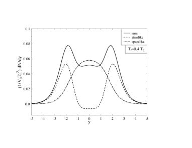
Figure 2: Rapidity distribution of particles freezing out on the $T_{f.out}=0.4T_{0}$ isotherm in the Landau model. The solid line corresponds to all the contributions in formula 1, the dashed-dotted line represents contributions from space-like parts of the isotherm and the dashed line contributions from time-like parts be96 ; ri98 . In this last case, note the negative contributions at y=0.

In the code SPHERIO ag01 , it can be a 20% overestimate of particle number. There are some ways to avoid these violations but none is completely satisfying ma99 .

The second problem is the following: do particles really suddenly stop interacting when they reach a certain hypersurface? Intuitively no, this must happen over a mean free path. This is corroborated by results from simulations of microscopical modelsBra ; Sor ; Bas : the shape of the region where particles last interacted is generally not a sharp surface as assumed for sudden freeze outs. Some exceptions might be heavy particles in heavy systems or the phase transition hypersurface.

We postpone the discussion of the second problem to section 4 and turn to the first problem.

II.2 2.2 Improved freeze out

In this section, we adopt the sudden freeze out picture and seek ways to incorporate conservation laws ma99 .

We suppose that prior to crossing the freeze out surface $\sigma$, particles have a thermalized distribution function and we know the baryonic current and energy momentum tensor, $n_{0}^{\mu}$ and $T_{0}^{\mu\nu}$. We suppose also that after crossing the surface, the distribution function is

$$f^{*}_{FO}(x,p;d\sigma^{\mu})=f_{FO}(x,p)\Theta(p^{\mu}\ d\sigma_{\mu})$$ (2)

The $\Theta$ function selects among particles which are emitted only only those with $d\sigma_{\mu}p^{\mu}>0$. This equation is solved in the rest frame of the gas doing freeze out (RFG) in figure 3 . We see that according to the value of $v={d\sigma_{0}/d\sigma_{x}}_{RFG}$, a region more or less big in the $p_{\perp}-p^{x}$ space can be excluded.

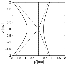
Figure 3: The solution to the equation $d\sigma_{\mu}p^{\mu}=0$ for $v$ = 0,65, 0 and -0,35 is given by the left hyperbola, the vertical axis and right hyperbola respectivaly. The permitted region is localized to the right of the curve in each of these three cases. The dashed lines correspond to the case of massless particles.

We do not know what the shape of $f_{FO}(x,p)$ is. To simplify, we first suppose that

$$f_{FO}(x,p)=\frac{1}{(2\pi)^{3}}exp\left(\frac{-p_{\mu}u^{\mu}+\mu}{T}\right)$$ (3)

with $u^{\mu}=\gamma(1,v,0,0)$ and $\mu$ is the baryonic potential.
This does not mean that $f_{FO}$ is thermalized but simply that we choose a parametrization of the thermalized type. This parametrization is arbitrary, we discuss later how to improve our ansatz. For the moment we use it to illustrate how to proceed in order not to violate conservation laws when using the Cooper-Frye formula.

It is possible to find expressions for the baryonic current, energy momentum tensor and entropy current corresponding to 2 in terms of Bessel-like functions and for massless particules, even analytical expressions as function of $v$, $T$ e $\mu$ ma99 .

To determine the parameters $v$,T and $\mu$ for matter on the post-freeze out side of $\sigma$, we need to solve the conservation equations

$[N^{\mu}d\sigma_{\mu}]=0\,\,\,\,\,\,\,\,[T^{0\mu}d\sigma_{\mu}]=0\,\,\,\,\,\,\,\,[T^{x\mu}d\sigma_{\mu}]=0$,

as function of quantities for matter on the pre-freeze out side, $v_{0}$, $T_{0}$ e $\mu_{0}$. This being done, we still need to check that

$[S^{\mu}d\sigma_{\mu}]\geq 0$ or $R=\frac{S^{\mu}d\sigma_{\mu}}{S_{0}^{\mu}d\sigma_{\mu}}\geq 1$

i.e. entropy can only increase when crossing $\sigma$. Generally, these equations need to be solved numerically but for massless particles, they have an analytical solution ma99 . For illustration, we show this solution for the case of a plasma with an MIT bag equation of state in figure 4.

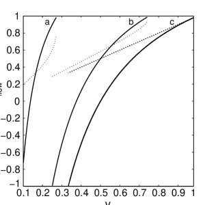
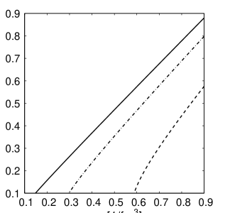
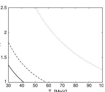
Figure 4: Solution of conservation laws in the case of a plasma.
Top: $v$ as function of $v_{0}$ (solid line) for a) $n_{0}=1.2\,fm^{-3},T_{0}=60\,MeV,\Lambda_{B}\equiv B^{1/4}=225\,MeV$, b) $n_{0}=0.1\,fm^{-3},T_{0}=60\,MeV,\Lambda_{B}=80\,MeV$, c) $n_{0}=1.2\,fm^{-3},T_{0}=60\,MeV,\Lambda_{B}=0\,MeV$. (Dashed lines: velocity of pos-freeze out baryonic flow).
Middle: baryonic density $n$ as function of $n_{0}$ for $v_{0}=0.5$, $T_{0}=50\,MeV$, a) $\Lambda_{B}=80\,MeV$ (continuous line), b) $\Lambda_{B}=120\,MeV$ (dashed-dotted line), c) $\Lambda_{B}=160\,MeV$ (dashed line).
Bottom : $R$, ratio of entropy currents for post and pre-freeze matter as function of $T_{0}$ for a) $n_{0}=0.1\,fm^{-3},v_{0}=0.5\,MeV,\Lambda_{B}=80\,MeV$ (solid line), b) $n_{0}=0.5\,fm^{-3},v_{0}=0.5\,MeV,\Lambda_{B}=80\,MeV$ (dashed line), c) $n_{0}=1.2\,fm^{-3},v_{0}=0.5\,MeV,\Lambda_{B}=225\,MeV$ (dotted line).

An interesting result can be seen on the top figure. Normally when using a Cooper-Frye formula, the velocity of matter pre and post freeze out is assumed to be the same. However in the figure, one sees that when imposing conservation laws, matter may be acelerated in a subtantial way. For example in case a), $v_{0}=0.2$ implies $v_{flow}=0.4$ and $v=0.6$. In term of effective temperature, there was an increase of 60%.

This example illustrates the importance of taking into account conservation laws when crossing $\sigma$. However, the choice of $f_{FO}$ as being parametrized in the same way as a thermalized distribution is arbitrary as we mentioned already. So we now study a more physical way of computing this function.

Consider an infinite tube with the $x<0$ part filled with matter and the $x>0$ part empty. At t=0, we remove the partition at $x=0$ and matter expands in vacuum. Suppose we remove the particles on the right hand side and put them back on the left hand side continuously so as to get a stationary flow, with a rarefaction wave propagating to the left of the matter.

In the spirit of the continuous emission model presented below, the distribution function of matter has two components, $f_{free}$ and $f_{int}$. Suppose that $f_{free}(x=0,p)=0$ and $f_{int}(x=0,p)=f_{therm}((x=0,p)$. A simple model for the fluid evolution is

$$\partial_{x}f_{int}(x,\vec{p})dx = -\Theta(p^{\mu}d\hat{\sigma}_{\mu})\frac{\cos\theta_{\vec{p}}}{\lambda}f_{int}(x,\vec{p})dx,\$$

$$\partial_{x}f_{free}(x,\vec{p})dx = +\Theta(p^{\mu}d\hat{\sigma}_{\mu})\frac{\cos\theta_{\vec{p}}}{\lambda}f_{int}(x,\vec{p})dx.$$ (4)

where $\cos\theta_{\vec{P}}=\frac{p_{x}}{p}$ in the rest frame of the rarefaction wave. A solution for these equations is

$$f_{int}(x,\vec{p})=f_{therm}(x=0,\vec{p})\exp\left[-\Theta(p^{\mu}d\hat{\sigma}_{\mu})\frac{\cos\theta_{\vec{p}}}{\lambda}x\right].$$ (5)

and

$$f_{free}(x,\vec{p}) = f_{therm}(x=0,\vec{p})\times$$ (6)

$$\left\{1-\exp\left[-\Theta(p^{\mu}d\hat{\sigma}_{\mu})\frac{\cos\theta_{\vec{p}}}{\lambda}x\right]\right\}$$

$$= f_{therm}(x=0,\vec{p})-f_{int}(x,\vec{p})$$

We see that $f_{free}$ tends to the cut thermalized distribution we saw above when $x\longrightarrow\infty$. In this model, the particle density does not change with $x$ but particles with $p^{\mu}d\hat{\sigma}_{\mu}>0$ pass gradually from $f_{int}$ to $f_{free}$.

To improve this model, we consider

$$\partial_{x}f_{int}(x,\vec{p})dx = -\Theta(p^{\mu}d\hat{\sigma}_{\mu})\frac{\cos\theta_{\vec{p}}}{\lambda}f_{int}(x,\vec{p})dx$$ (7)

$$+\left[f_{eq}(x,\vec{p})-f_{int}(x,\vec{p})\right]\frac{1}{\lambda^{\prime}}dx,$$

$$\partial_{x}f_{free}(x,\vec{p})dx=+\Theta(p^{\mu}d\hat{\sigma}_{\mu})\frac{\cos\theta_{\vec{p}}}{\lambda}f_{int}(x,\vec{p})dx.$$ (8)

The additional term in $f_{int}$ includes the tendency for this function to tend towards an equilibrium function due to collisions with a relaxation distance $\lambda^{\prime}$. Due to the loss of energy, momentum and particle number, $f_{eq}$ is not the initial thermalized function but its parameters $n_{eq}(x)$, $T_{eq}(x)$ and $u^{\mu}_{eq}(x)$ can be determined using conservation laws. In the case of immediate re-thermalization ($f_{int}=f_{eq}$), for a gas of massless particles with zero net baryon number, the solution is shown in figure 5.

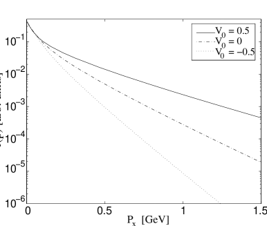
Figure 5: $f_{free}(p_{x})$ ( equivalent to the $f^{*}_{FO}$ in the previous section), computed at $p_{y}=0,x=100\lambda,T_{0}=130\,MeV$.

One sees that the solution $f_{free}$ is not a thermalized type cut function.

Even more importantly, this distribution exibits a curvature which reminds the data on $p_{\perp}$ distribution for pions. Other explaination for this curvature are transverse expansion or resonance decays. On the basis of our work, it is difficult to trust totally analyses which extracts thermal freeze out temperatures and fluid velocities using only transverse expansion and resonance decays.

More details and improvement on how to compute the post freeze out distribution function were presented in various papers an99 ; ma99b ; ma03 ; cs04 ; ta04 .

Finally, it is interesting to note that models that combine hydrodynamics with a cascade code also suffer from the problem of non-conservation of energy-momentum and charge tea01 or inconsistency du00 , as discussed in bu03 .

III 3. Separate freeze outs

In this section, we suppose that the sudden freeze out picture can be used and see how well it describes data.

III.1 3.1 Chemical freeze out

Strangeness production plays a special part in ultrarelativistic nuclear collisions since its increase might be evidence for the creation of quark gluon plasma. Many experiments therefore collect information on strangeness production.

We can consider for example the results obtained by the CERN collaborations WA85 (collision S+W), WA 94 (collision S+S) and WA97, later on NA57 (collision Pb+Pb). One can combine various ratios to obtain a window for the freeze out conditions compatible with all these data. The basic idea is simple, for example:

$$\overline{\Lambda}/\Lambda\sim\exp\frac{2(\mu_{S}-\mu_{B})}{T}_{|f.out}=exp.\,value.$$ (9)

(neglecting decays.)

In principle, this equation depends on three variables. However, supposing that strangeness is locally conserved, this leads to a relation $\mu_{S}(\mu_{b},T)$, then given a minimum and a maximum values, the above equation gives a relation $T_{f.out}(\mu_{B\,f.out})$. We show typical results in figure 6.

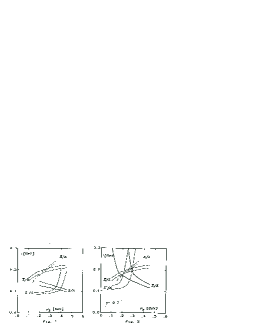
Figure 6: Search of a window re94 of values of $T_{f.out}$ e $\mu_{b,\,f.out}$ reproducing WA85 data. This window only exists for $\gamma<1$ (for this reference).

The parameter $\gamma$ in this figure is basically a phenomenological factor, which indicates how far from chemical equilibrium we are, it is introduced in front of the factors $e^{\pm\mu_{s}/T}$ where $\mu_{s}$ is the s quark chemical potential, $\mu_{s}=\mu_{B}/3-\mu_{S}$. (There exists a study by C.Slotta et al. cl95 motivating this way of including $\gamma$.) It can be seen that if $\gamma=0,7$ it is possible to reproduce the experimental ratios $\overline{\Lambda}/\Lambda$, $\overline{\Xi}/{\Xi}$, $\Xi/\Lambda$, $\overline{\Xi}/\overline{\Lambda}$ choosing $T_{f.out}$ and $\mu_{b,\,f.out}$ in a certain window. This window is located around $T_{f.out}\sim 180-200$ MeV, $\mu_{b,\,f.out}\sim 200-300$ MeV. One can be surprised by such high values since particle densities are still high. However these results are rather typical as can be checked in the table  1.

Table 1: Summary of freeze out values from J.Sollfrank so97a .

collision	T (MeV)	$\mu_{b}$ (MeV)	$\gamma_{s}$	ref.
S+S	170	257	1	Davidson91a
	197$\pm$29	267$\pm$21	1.00$\pm$0.21	so94
	185	301	1	tawai96
	192$\pm$15	222$\pm$10	1	panagiotou96
	182$\pm$9	226$\pm$13	0.73$\pm$0.04	becattini97
	202$\pm$13	259$\pm$15	0.84$\pm$0.07	so97b
S+Ag	191$\pm$17	279$\pm$33	1	panagiotou96
	180.0$\pm$3.2	238$\pm$12	0.83$\pm$0.07	becattini97
	185$\pm$8	244$\pm$14	0.82$\pm$0.07	so97b
S+Pb	172$\pm$16	292$\pm$42	1	andersen94
S+W	190$\pm$10	240$\pm$40	0.7	re94
	190	223$\pm$19	0.68$\pm$0.06	letessier95
	196$\pm$9	231$\pm$18	1	braun96
S+Au(W,Pb)	165$\pm$5	175$\pm$5	1	panagiotou96
	160	171	1	spieles97
	160.2$\pm$3.5	158$\pm$4	0.66$\pm$0.04	so97b

The explaination usually given nowadays is that at these temperatures, particles are doing a chemical freeze out, they stop having inelastic collisions and their abundances are frozen.

III.2 3.2 Thermal freeze out

Transverse mass distributions obtained experimentally (when plotted logarithmically) exhibit large inverse inclinations. These are called effective temperatures.

In the case of hydrodynamics, these effective temperatures are thought to be due to the convolution of the fluid temperature with its transverse velocity, both at freeze out. So in particular the effective temperatures are higher than the fluid temperature. In addition, the effective temperature should be larger the larger the particle mass is , since the “kick” received in momentum, $\sim mv^{fluid}_{f.out}$, due to transverse expansion, is larger (this argument is only valid for the non-relativistic part of the spectrum i.e. $p_{\perp}<<m$; the effective temperature does not depend on mass for the part of the spectrum where $p_{\perp}>>m$ (but for that part of the spectra other phenomena might be important). In general, given an experimental $m_{\perp}$ spectrum, there exist many pairs of $T_{f.out}$ and $v^{fluid}_{f.out}$ which can reproduce it.

To remove this ambiguity, we can compare the $m_{\perp}$ spectra for various types of particles (e.g. na44 ), or for a given type of particle, for example pions, combine the fit of the spectrum with results on HBT correlations (e.g. wi97 ). A compilation for various accelerator energies of values for $T_{f.out}$ obtained from particle spectra is presented in figure 7 (dashed line).

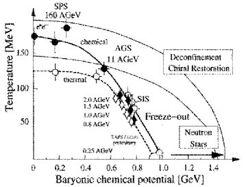
Figure 7: Phase diagram with lines indicating values of freeze out parameters at various energies obtained from particle abundances (solid line) and particle spectra (dashed line) he97 .

A typical value at SPS is $T_{f.out}\sim 125$ MeV. One can be surprised by the fact that these values for $T_{f.out}$ are lower than those obtained from particle ratios. The usual explaination for this is that 125 MeV corresponds to a thermal freeze out of particles, i.e. when they stop having elastic collisions and the shape of their spectra become frozen. This model with a chemical freeze out followed by a thermal freeze out is called separate freeze out model. Its parameters depend on the energy as shown in figure 7; the possible decrease of $T_{f.out}$ with increasing energy is discussed in ha91 ; na92 . Some possible problems of this model ($\Omega$ temperature and pion abundance are discussed later). For the moment let us see how to incorporate this description in hydrodynamics, since so far it was based only on the analysis of two different types of data with thermal or semi-analytical hydrodynamical models.

III.3 3.3 Is it quantitatively necessary to modify hydrodynamics to incorporate separate freeze outs?

In ar01 , we made a preliminary study of whether such a separate freeze out model would quantitatively influence the hydrodynamical expansion of the fluid. For this, we used a simple hydrodynamical model, with longitudinal expansion only and longitudinal boost invariance bj .

For a single freeze out, the hydrodynamical equations are

$$\frac{\partial\epsilon}{\partial t}+\frac{\epsilon+p}{t} = 0$$

$$\frac{\partial n_{B}}{\partial t}+\frac{n_{B}}{t} = 0$$ (10)

The last equation can be solved easily

$$n_{B}(t)=\frac{n_{B}(t_{0})t_{0}}{t}.$$ (11)

Given an equation of state, $p(\epsilon,n_{B})$, we can get $\epsilon(t)$ and $n_{B}(t)$, solving (10). From them, $T(t)$ and $\mu_{B}(t)$ can be extracted. So, if the freeze out criterion is $T_{f.out}=constant$, one can see which are the values for other quantities at freeze out, for example the values of $t_{f.out}$, $\mu_{B\,f.out}$, … These values being known, spectra can be computed.

Now let us start again with the previous model, but we suppose that when a certain temperature $T_{ch.f.out}$ is reached (corresponding to a certain $t_{ch.f.out}$) some abundances are frozen. To fix ideas, let us suppose that $\Lambda$ and $\bar{\Lambda}$ are in this situation. In this case, for $t\geq t_{ch.f.out}$, in addition to the hydrodinamic equations above, ( 10), we must introduce separate conservation laws for these two types of particles

$$\frac{\partial n_{\Lambda}}{\partial t}+\frac{n_{\Lambda}}{t} = 0$$ (12)

$$\frac{\partial n_{\bar{\Lambda}}}{\partial t}+\frac{n_{\bar{\Lambda}}}{t} = 0.$$ (13)

Again it is easy to solve these equations

$$n_{\Lambda}(t) = \frac{n_{\Lambda}(t_{0})t_{0}}{t}$$ (14)

$$n_{\bar{\Lambda}}(t) = \frac{n_{\bar{\Lambda}}(t_{0})t_{0}}{t}$$ (15)

For times $t\geq t_{ch.f.out}$, we need to solve the hydrodynamic equations ( 10) with an equation of state modified to incorporate these conserved abundances.

We suppose that the fluid is a gas of non-interacting resonances.

$$n_{i} = \frac{g_{i}m_{i}^{2}T}{2\pi^{2}}\sum_{n=1}^{\infty}(\mp)^{n+1}\frac{e^{n\mu_{i}/T}}{n}K_{2}(nm_{i}/T)$$ (16)

$$\epsilon_{i} = \frac{g_{i}m_{i}^{2}T^{2}}{2\pi^{2}}\sum_{n=1}^{\infty}(\mp)^{n+1}\frac{e^{n\mu_{i}/T}}{n^{2}}[3K_{2}(nm_{i}/T)$$

$$+ \frac{nm_{i}}{T}K_{1}(nm_{i}/T)]$$

$$p_{i} = \frac{g_{i}m_{i}^{2}T^{2}}{2\pi^{2}}\sum_{n=1}^{\infty}(\mp)^{n+1}\frac{e^{n\mu_{i}/T}}{n^{2}}K_{2}(nm_{i}/T)$$ (18)

where $m_{i}$ is the particle mass, $g_{i}$, its degeneracy and $\mu_{i}$, its chemical potential, the minus sign holds for fermions and plus for bosons. In principle each particle species $i$ making early chemical freeze-out has a chemical potential associated to it; this potential controls the conservation of the number of particles of type $i$. For particle species not making early chemical freeze-out, the chemical potential is of the usual type, $\mu_{i}=B_{i}\mu_{B}+S_{i}\mu_{S}$, where $\mu_{B}$ ($\mu_{S}$) ensures the conservation of baryon number (strangeness) and $B_{i}$ ($S_{i}$) is the baryon (strangeness) number of particle of type $i$. So the modified equation of state depends not only on $T$ and $\mu_{B}$ but also $\mu_{\Lambda}$, $\mu_{\bar{\Lambda}},etc$. (the notation “$etc$” stands for all the other particles making early chemical freeze-out). This complicates the hydrodynamical problem, however we can note the following.

If $m_{i}-\mu_{i}>>T$ (the density of type $i$ particle is low) and $m_{i}>>T$, (these relations should hold for all particles except pions and we checked them for various times and particle types) the following approximations can be used

$$n_{i} = \frac{g_{i}}{2\pi^{2}}\sqrt{\frac{\pi}{2}}(m_{i}T)^{3/2}e^{(\mu_{i}-m_{i})/T}$$ (19)

$$\times\left(1+\frac{15T}{8m_{i}}+\frac{105T^{2}}{128m_{i}^{2}}+...\right)$$

$$\epsilon_{i} = n_{i}m_{i}\left(1+\frac{3T}{2m_{i}}+\frac{15T^{2}}{8m_{i}^{2}}+...\right)$$ (20)

$$p_{i} = n_{i}T$$ (21)

We note that $\epsilon_{i}$ and $p_{i}$ are written in term of $n_{i}$ and T. Therefore we can work with the variables $T,\mu_{B},n_{\Lambda},n_{\bar{\Lambda}},etc$, rather than $T,\mu_{B},\mu_{\Lambda},\mu_{\bar{\Lambda}},etc$. The time dependence of $n_{\Lambda},n_{\bar{\Lambda}},etc$ is known as discussed already. So the modified equation of state can be computed from $t$, $T$ and $\mu_{B}$.

In figure 8, we compare the behavior of $T$ and $\mu_{B}$ as function of $t$, obtained from the hydrodynamical equations using the modified equation of state and the unmodified one.

Figure 8: $\mu_{B}$ and T as function of time in the case where all particles have simultaneous freeze-outs (dashed line) and (I) all strange particles in basic multiplets make an early chemical freeze-out (continuous line), (II) all strange particles except $K$ and $K^{*}$’s make an early chemical freeze-out (dotted line).

We see that if the chemical and thermal freeze-out temperatures are very different or if many particle species make an early chemical freeze out, the thermal freeze out time is quite affected. Therefore it is important to take into account the effect of the early chemical freeze-out on the equation of state to make predictions for observables which depend on thermal freeze-out volumes (which are related to the thermal freeze out time), for example particle abundances and eventually particle correlations.

If the chemical and thermal freeze-out temperatures are not very different or if few particle species make the early freeze out, one can proceed as follows. One can use an unmodified equation of state in a hydrodynamical code and to account for early chemical freeze-out of species $i$, when the number of type $i$ particles was fixed, use a modified Cooper-Frye formula

$$\frac{Ed^{3}N_{i}}{dp^{3}}=\frac{N_{i}(T_{ch.f.})}{N_{i}(T_{th.f.})}\times\int_{S_{th.f.}}d\sigma_{\mu}p^{\mu}f(x,p).$$ (22)

The second factor on the right hand side is the usual one and it gives the shape of the spectrum at thermal freeze-out, the first factor is a normalizing term introduced such that upon integration on momentum $p$, the number of particles of type $i$ is $N_{i}(T_{ch.f})$. As an illustration, using HYLANDER-PLUS nel , we show in figure 9 that both the shapes of $m_{\perp}$ spectra and abundances can be reproduced for $T_{ch.f.}=176$ MeV and $T_{th.f.}=139$ MeV, while simultaneous freeze-outs at $T_{ch.f.}=T_{th.f.}=139$ MeV would yield the correct shapes but too few particles.

Figure 9: $m_{\perp}$ spectra: NA49 data and HYLANDER-PLUS results. Dashed-dotted curves: single freeze out at $T_{f.out}=139MeV$. Solid curves (resp. dashed): chemical freeze out at $T_{f.out.\,ch.}=$ 176 (resp. 184) MeV and thermal freeze out at $T_{f.out.\,th.}=$ 139 MeV (see text).

Hirano and Tsuda hi confirmed the importance of including separate freeze outs in hydrodynamical codes, in particular they studied elliptic flow and HBT radii at RHIC. This is also consistent with results in teaney .

IV 4. Continuous emission

IV.1 4.1 Formalism and modified fluid evolution

In this section, we present a possible way out of the second problem mentioned above. In colaboration with Y.Hama and T.Kodama, I made a description of particle emission Grassi95a ; Grassi96a which incorporates the fact that they, at each instant and each location, have a certain probability to escape without collision from the dense medium (said in the same terms as above: there exists a region in spacetime for the last collisions of each particle). So the distribution function of the system in expansion has two terms $f_{free}$, representing particles that made their last collision already, and $f_{int}$, corresponding to the particles that are still interacting

$$f(x,p)=f_{free}(x,p)+f_{int}(x,p)$$ (23)

The formula for the free particle spectra is given by

$$Ed^{3}N/dp^{3}=\int d^{4}x\,D_{\mu}[p^{\mu}f_{free}(x,p)]$$ (24)

(neglecting particles that are initially free; note that if it were not the case, the use of hydrodynamics would not be possible). $D_{\mu}$ indicates a four-divergence in general coordinates. This integral must be evaluated for the whole spacetime occupied by the fluid.

This way, we see that the spectra contains information about the whole fluid history and not just the time when it is very diluted. (This formula reduces to the Cooper-Frye formula (1) in an adequate limit).

We can write

$$f_{free}={\cal P}f={\cal P}/(1-{\cal P})f_{int}.$$ (25)

${\cal P}(x,p)=f_{free}/f$, the fraction of free particles, can be identified with the probability that a particle of momentum $p$ escapes from $x$ without collisions, so to compute this quantity we use the Glauber formula

$${\cal P}(x,p)=exp\left(-\int_{t}^{\infty}n(x^{\prime})\sigma v_{rel}dt^{\prime}\right).$$ (26)

We suppose also that all interacting particles are thermalized, so

$$f_{int}(x,p) = f_{th}(x,p)=g/(2\pi)^{3}$$ (27)

$$\times 1/\{\exp[(p.u(x)-\mu(x))/T(x)]\pm 1\},$$

where $u^{\mu}$ is the fluid velocity, $\mu$ its chemical potential ($\mu=\mu_{B}B+\mu_{S}S$ with $B$ the baryonic number of the hadron, $S$, its strangeness and $\mu_{B}$ and $\mu_{S}$ the associated chemical potentials) and $T$ its temperature at $x$.

To compute $u^{\mu}$, $\mu$ and $T$, we must solve the equations of conservation of energy-momentum and baryonic number

$$D_{\mu}T^{\mu\,\nu} = 0$$ (28)

$$D_{\mu}(n_{b}u^{\mu}) = 0.$$ (29)

In the figure 10, examples of solution are given. We can see that the fluid evolution with continuous emission is different from the usual case without continuous emission. For example, and as expected, the temperature decreases faster since free particles carry with them part of the energy-momentum.

In principle we have all the ingredients to compute (24). However there exist two problems: 1) numerically, in the equation 25 we can have divergencies if ${\cal P}$ goes faster to 1 than $f_{int}$ goes to zero 2) the hypothesis that $f_{int}$ is termalized (cf. eq.(27)) must loose its validity when ${\cal P}$ goes to 1. To avoid this problem, we divide space-time in eq. (24), in two regions: the first with ${\cal P}>{\cal P_{F}}$ and the second with ${\cal P}\leq{\cal P_{F}}$, for some reasonable value of ${\cal P_{F}}$. Using Gauss theorem, the second part reduces to an integral over the surface ${\cal P}={\cal P_{F}}$ (which depends on the particle momentum)

$$I_{1} = \int_{{\cal P}={\cal P_{F}}}d\sigma_{\mu}p^{\mu}f_{free}$$ (30)

$$= \frac{{\cal P_{F}}}{1-{\cal P_{F}}}\int_{{\cal P}={\cal P_{F}}}d\sigma_{\mu}p^{\mu}f_{th}$$ (31)

There is still a certain fraction of interacting particles, $1-{\cal P_{F}}$ of the total, on this surface, it is these particles which in principle turn free in the region ${\cal P}>{\cal P_{F}}$. To count them, we suppose that they are rather diluted (i.e. ${\cal P_{F}}$ is rather large) and we can apply a Cooper-Frye formula for them

$$I_{2} \sim \int_{{\cal P}={\cal P_{F}}}d\sigma_{\mu}p^{\mu}f_{int}$$ (32)

$$= \int_{{\cal P}={\cal P_{F}}}d\sigma_{\mu}p^{\mu}f_{th}$$ (33)

So finally

$$E\frac{d^{3}N}{dp^{3}}=I_{1}+I_{2}\sim\frac{1}{1-{\cal P_{F}}}\int_{{\cal P}={\cal P_{F}}}d\sigma_{\mu}p^{\mu}f_{th}.$$ (34)

It is this formula which is used below, with ${\cal P_{F}}=0.5$ (but we tested the effect of changing this value) and coordinates adequate for the geometry of the problem. It is similar to a Cooper-Frye formula (1), however one must note that the condition ${\cal P}={\cal P_{F}}$ depends not only on the localization of a particle but its momentum, which as we will see has interesting consequences.

Figure 10: Fluid evolution supposing longitudinal boost invariencebj . Top two: for a light projectile such as S, $T$ and $\mu_{B}$ as function of radius; as a first approximation transverse expansion is neglected. ( Solid lines correspond to a fluid with continuous emission, dashed line lines to a fluid without continuous emission, i.e. the usual case.) Bottom three: for a heavy projectile such as Pb, $T$, $\mu_{B}$ and fluid velocity as function of radius; transverse expansion is included (times: 1,4,7,10 fm).

IV.2 4.2 Comparison of the continuous emission and freeze out scenarios

In this section, I compare the interpretation of experimental data in both models.

a. Strange particle ratios
We saw above that for the freeze out mechanism, strange particle ratios give information about chemical freeze out. Now we see how to interpret these data within the continuous emission sceanrio Grassi96c ; Grassi97 ; Grassi98 ; Grassi99a ; Grassi99b . In this case, the only parameters are the initial conditions $T_{0}$ e $\mu_{b\,0}$ and a value that we suppose average for $\gamma$. We therefore fix a set of them, solve the equations of hydrodinamics with continuous emission, compute and integrate in $p_{\perp}$ the spectra given by (34) for each type of particles (we include also the decays of the various types of particles in one another). In a way similar to freeze out but now with initial values instead of freeze out values, we get in figure 11, a window of initial conditions which permits to reproduce the various experimental ratios. (We also look at other ratios than those shown in the figure, tested the effect of changes in the equation of state, cross section, initial time, type of experimental cutoff.)

Figure 11: Window in initial conditions allowing to reproduce WA85 data, for an equation of state with excluded volume corrections Grassi98 .

We see therefore that the initial conditions necessary to reproduce the WA85 data are

$$T_{0}\sim\mu_{b\,0}\sim 200\,MeV$$ (35)

These values may seem high for the existence of a hadronic phase, lattice gauge QCD simulations seem to indicate values smaller for the quark-hadron transition. Here we can note that 1) values of QCD on the lattice are still evolving (problems exist to incorporate quarks with intermediate mass, include $\mu_{b}\neq 0$, etc. 2) Our own model is still being improved and we know for example that the equation of state affects the localization of the window in initial conditions compatible with data.

In figure 12, the same kind of analysis was done for the data WA97.

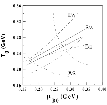
Figure 12: Window in initial conditions reproducing WA97 data in the case of an equation of state without excluded volume corrections. With volume corrections, the window is lower Grassi99b .

With the reservation in the caption of the figure, we see that the initial conditions are not very different from the one above.

We can therefore conclude that the interpretation of data on particle ratios lead to totally different information according to the emission model used. For the freeze out model, we get information about chemical freeze out while for continuous emission, we learn about the initial conditions.

b. Transverse mass spectra
For freeze out, we saw that these spectra tell us about thermal freeze out (temperature and fluid velocity). Now for continuous emission let us see how to interpret these same spectra Grassi96c ; Grassi97 ; Grassi98 ; Grassi99a ; Grassi99b . In this case, the initial conditions were already determined from strange particle ratios, they cannot be changed and must be used to compute the spectra as well. For example, in figure 13, various spectra are shown, assuming $T_{0}=\mu_{b\,0}=200$ MeV, and compared with experimental data.

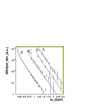
Figure 13: Using longitudinal boost invariance and no transverse expansion, we compare our predictions, top to bottom, with NA35 data (S+S, all rapidity), with WA94 data (S+S, midrapidity, large transverse momenta) and with WA85 data (S+W, midrapidity, large transverse momenta) Grassi99a .

This comparison should not be considered as a fit but as a test of the possibility of interpreting various types of data in a self-consistent way with continuous emission (in particular note that our calculations were done assuming longitudinal boost invariance).

We learn various information from this comparison. In these figures, we do not take into account transverse expansion. With the S+S NA35 data, we note that the heavy particles and high transverse momentum pions have similar inverse inclinations $T_{0}\sim 200$ MeV. The particles heavier than pions, due to termal suppression, are mainly emitted early when the temperature is $\sim T_{0}$. For lower temperatures, there are still emitted (and more easily due to matter dilution) but their densities are quite smaller (this is what is called thermal suppression) and their contributions as well. The high transverse momentum pions have large velocity and (if not too far away from the outer fluid surface) escape without collision earlier than pions at the same place but with smaller velocity, so these high transverse momentum pions also escape at $\sim T_{0}$. Pions are small mass particles and are little affected by thermal suppression. This way, they can escape in significative number at various temperatures. This is reflected by their spectra, precisely its curvature. (In our calculation, decays into pions are not included, this would fill the small transverse momentum region and improve the agreement with experimental data.)

The S+S WA94 data also indicate that continuous emission is compatible with data. Finally, the S+W WA85 data seem to indicate that perhaps somewhat different initial conditions or a little of transverse expansion might be necessary to reproduce data.

Our calculations including transverse expansion indicate that little transverse expansion is compatible with data for light projectile. This is understandable noting that the effective temperature of spectra are already of order the initial temperature $\sim$ 200 MeV. In the case of heavy projectile, the situation is different. The various types of particles have different temperatures, all well above 200 MeV. In this case, we must include transverse expansion to get consistency with data. An example is shown in figure 14 with the same values of $T_{0}$ and $\mu_{b,0}$ than previously, 200 MeV.

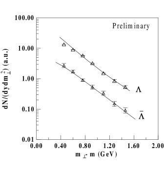
Figure 14: WA97 data and example of comparison with continuous emission with transverse expansion (not a least square fit) for $T_{0}=\mu_{b.0}=200$ MeV Grassi99b .

c. The case of the $\Omega$
The effective temperatures in the case of heavy projectiles, particularly for the $\Omega$, have attracted a lot of attention for the following reason. In the usual hydrodynamics with freeze out, as we saw, it is expected that effective temperatures increase with mass. In this context it was difficult to understand why the $\Omega$ had an effective temperature much lower than other particles in figure 15.

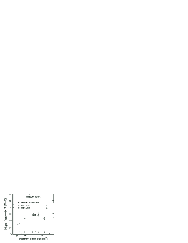
Figure 15: Compilation of experimental data on effective temperatures in the case of heavy projectile and predictions for usual hydrodynamics va98 . (The various experiments have different rapidity and transverse momentum cutoffs). In general, deuteron is left outside the hydrodynamical analysis: it is little bounded and should form later in the fluid evolution from coalescence of a neutron and a proton with similar moment.

.

A possible explaination within hydrodynamics with separate freeze outs, is that the $\Omega$ made its chemical and thermal freeze out together, early. Van Hecke et al. va98 argued that this is reasonable since it is expected that $\Omega$ has a small cross section (because there is no channel for $\Omega\pi\rightarrow resonance\rightarrow\Omega\pi$) and showed that the microscopical model RQMD can reproduce the data.

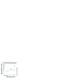
Figure 16: Predictions from RQMD va98 in the same experimental situation as the previous figure.

In our model originally we had used the same value of the cross sections to compute the escape probability for the various types of particles. This is not expected and indeed in this case, continuous emission, does not lead to good predictions as shown in figure 17a.

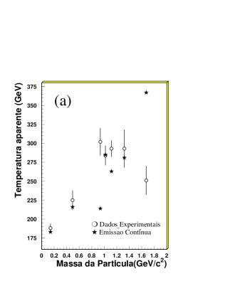
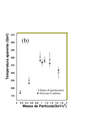
Figure 17: Comparison of experimental data on effective temperatures in the case of a heavy projectile with predictions from continuous emission. Top: all cross section supposed equal. Bottom: more realistic cross section values (cf. text) os99 ; Grassi99b .

Therefore in the spirit of microscopic models, we also show our predictions in figure 17b, for continuous emission and the following cross sections: $\sigma_{\pi\pi}\sim<\sigma v_{rel}>_{\pi\pi}\sim 1fm^{2}$, $\sigma_{N\pi}\sim<\sigma v_{rel}>_{N\pi}\sim 3/2<\sigma v_{rel}>_{\pi\pi}$ (using additive quark model estimate), $\sigma_{\Lambda\pi}\sim<\sigma v_{rel}>_{\Lambda\pi}\sim 1,2<\sigma v_{rel}>_{\pi\pi}$ (using additive quark model estimate ba98 ) and $\sigma_{\Omega\pi}\sim<\sigma v_{rel}>_{\Omega\pi}\sim 1/2<\sigma v_{rel}>_{N\pi}$ (using estimate in bravina98b ). The predictions now are in agreement with data. However, the cross sections are poorly known and our results are sensitive to their values.

Recently, with new data by NA49, WA97 WA97art and NA49 NA49art came to the conclusion that in fact there is no need for early joint chemical and thermal freeze outs for the $\Omega$: all their spectra can be fitted with a simple hydro inspired model as seen in figure 18. The previous difficulty for WA97 came from the fact heinzart that $\Omega$ was observed at high $p_{\perp}$. However now, STAR has problems starart to fit with a simple hydro inspired model the $\Xi$ together with $\pi,p,K,\Lambda$ and would need to assume early joint chemical and thermal freeze outs for the $\Xi$, as shown in figure 19. More recently, it has been noted na49omega by NA49, that their conclusion depends on the parametrization used and in na57omega , NA57 argues that due to low statistics, it is not clear what conclusion can be drawn for the $\Omega$. In fgsqm , an attempt was made to reproduce with a single thermal freeze out temperature in a hydrodynamical code, all transverse mass spectra at a given energy.

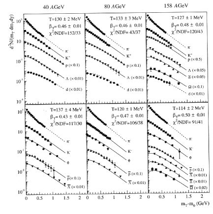
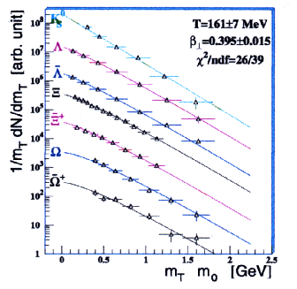
Figure 18: Data and hydro inspired fit for all particles including $\Omega$, top, NA49 and bottom, NA57 WA97art ; NA49art .

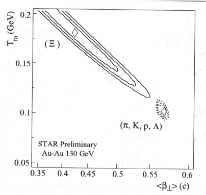
Figure 19: A hydro fit to transverse mass spectra leads to high $T_{f.out}$ for $\Xi$ and lower for $\pi,p,K,\Lambda$ starart .

d. Pion abundances
We showed that strange particle ratios can be reproduced by a model with chemical freeze out around 180 MeV. The abundances too can be reproduced. The problem is that the pion number is too low. This was noticed by Davison et al. Davidson92a , as shown in their table 2 reproduced below

Table 2: Comparison between NA35 data and previsions from a thermal model Davidson92a .

	$K_{S}^{0}$	$K^{+}$	$K^{-}$	$\Lambda$	$\overline{\Lambda}$	“p’	$\pi^{-}$
Th.	10.7	14.2	7.15	8.2	1.5	23.2	56.9
Exp.	10.7	12.5	6.9	8.2	1.5	22.0	92.7
	$\pm$2.0	$\pm$0.4	$\pm$0.4	$\pm$0.9	$\pm$0.4	$\pm$2.5	$\pm$4.5

There are various ways to try to solve this problem.

1. It can be argued (in a spirit similar to Cleymans et al. cl93 ) that strange particles do their chemical freeze our early around 180 MeV and their thermal freeze out around 140 MeV but the pions do their chemical and thermal freeze outs together around 140 MeV. In fact Ster et al. st99 manage to reproduce data by NA49, NA44 and WA98 on spectra (including normalization i.e. abundances) for negatives, pions, kaons and protons and HBT radii (see next section) with temperature around 140 MeV and null chemical potential for the pions. On the other side, Tomásik et al. to99 say that for the same kind of objective, they need temperatures of order 100 MeV and non zero chemical potential for the pions. So it is not clear if to reproduce the pion abundance, it is necessary to modify the hydrodynamics with separate freeze out, including pions out of chemical equilibrium or not.

2. Gorenstein and colaborators ri97 ; ye97 ; ye99 studied modifications of the equation of state, precisely they included a smaller radius for the volume corrections of the pion.

3. Letessier et al. made a série of papers le93 ; letessier95 arguing that the large pion abundance is indicative of the formation of a quark gluon plasma hadronizing suddenly, with both strange and non-strange quarks out of chemical equilibrium le98 .

Given the difficulty that freeze out models have with pions, it is interesting to compute abundances with continuous emission models. In the table, results and NA35 data from S+S are shown (data are selected at midrapidity).

Table 3: Comparison between experimental data, results for continuous emission at $T_{0}=\mu_{b,0}=200$ MeV and freeze out at $T_{0}=\mu_{b,0}=T_{f.out}=\mu_{b\,f.out}=200$ MeV.

	experimental value	continuous emission	freeze out
$\Lambda$	1.26$\pm$0.22	0.96	0.92
$\bar{\Lambda}$	0.44$\pm$0.16	0.29	0.46
$p-\bar{p}$	3.2$\pm$1.0	3.12	1.32
$h^{-}$	26$\pm$1	27	15.7
$K^{0}_{S}$	1.3$\pm$0.22	1.23	1.06

It can be seen that in the continuous emission model, a larger number of pions is created. In Grassi00a , we related this increase to the fact that entropy increases during the fluid expansion. This is due to the continuous process of separation into free and interacting components as well as continuous re-termalization of the fluid. In contrast, in the usual hydrodynamic model, entropy is conserved and related to the number of pions; so in this usual model, observation of a large number of pions implies a large initial entropy and is indicative of a quark gluon plasma le93 ; letessier95 ; le98 . In our case, a large number of pions does not imply a large initial entropy and the existence of a plasma. It can be noted that the interpretation of data is quite influenced by the choice of the particle emission model.

e. HBT
Interferometry is a tool which permits extracting information on the spacetime structure of the particle emission source and is sensitive to the underlying dynamics. Since pion emission is different in freeze out and continuous emission models, it is interesting to compare their interferometry predictions (for a review see sandra ). This was done in ref. Grassi00b .

In this work, the formalism of continuous emission Grassi95a ; Grassi96a was extended to the computation of correlation functions. Precisely, we computed

$$C(k_{1},k_{2})=C(q,K)=1+\frac{|G(q,K)|^{2}}{G(k_{1},k_{1})G(k_{2},k_{2})}\;\;,$$ (36)

where $q^{\mu}=k_{1}^{\mu}-k_{2}^{\mu}$ e $K^{\mu}=\frac{1}{2}(k_{1}^{\mu}+k_{2}^{\mu})$.

In the case of freeze out (in the Bjorken model with pseudo-temperatureko86 )

$$G(k_{1},k_{2})=2<\frac{dN}{dy}>\{\frac{2}{q_{T}R_{T}}J_{1}(q_{T}R_{T})\}K_{0}(\xi)$$ (37)

where

$$\xi^{2} = [\frac{1}{2T}(m_{1T}+m_{2T})-i\tau(m_{1T}-m_{2T})]^{2}+$$ (38)

$$2\,(\frac{1}{4T^{2}}+\tau^{2})\,m_{1T}\,m_{2T}\,[\cosh(\Delta y)-1]\;\;,$$

$\Delta y=y_{1}-y_{2}$, $<\ >$ indicates average over particles 1 and 2
and

$$G(k_{i},k_{i})=2\frac{dN}{dy_{i}}K_{0}(\frac{m_{iT}}{T}).$$ (39)

In the case of continuous emission in the Bjorken model with pseudo-temperature

$$G(q,K) = \frac{1}{(2\pi)^{3}(1-{\bf{\cal P}}_{{\cal F}})}\int_{0}^{2\pi}d\phi\int_{-\infty}^{+\infty}d\eta$$

$$\times \{\int_{0}^{R_{T}}\rho\;d\rho\;\tau_{{\cal F}}\;M_{T}\;\cosh(Y-\eta)$$

$$\times e^{i[\tau_{{\cal F}}(q_{0}\cosh\eta-q_{L}\sinh\eta)-\rho q_{T}\cos(\phi-\phi_{q})]}$$

$$+ \!\int_{\tau_{0}}^{+\infty}\!\!\tau d\tau\rho_{{\cal F}}K_{T}\cos\phi$$

$$\times \,e^{i[\tau(q_{0}\cosh\eta-q_{L}\sinh\eta)-\rho_{{\cal F}}q_{T}\cos(\phi-\phi_{q})]}\}$$

$$\times e^{-M_{T}\cosh(Y-\eta)/T_{ps}(x)},$$

with $M_{T}=\!\sqrt{K_{T}^{2}+M^{2}},\;\vec{K}_{T}=\frac{1}{2}(\vec{k}_{1}+\vec{k}_{2})_{T}\,,\,M^{2}=K_{\mu}K^{\mu}=m^{2}-\frac{1}{4}q_{\mu}q^{\mu}$, $Y$ is the rapidity corresponding to $\vec{K}$, $\phi$ is the azimuthal angle in relation to the direction of $\vec{K}$ and $\phi_{q}$ is the angle between the directions of $\vec{q}$ and $\vec{K}$. $\tau_{\cal{P_{F}}}$ and $\rho_{\cal{P_{F}}}$ are determined by $\cal{P}=\cal{P_{F}}$. $T_{ps}(x)=1,42T(x)-12,7MeV$.

In Grassi00b , a few idealized cases were studied and then some cases more representative of the experimental situation, were presented. For example, instead of $C(q,K)$, we computed

$$\langle C(q_{L})\rangle=1+$$

$$\frac{\int_{-180}^{180}dK_{L}\int_{50}^{600}dK_{T}\int_{0}^{30}dq_{S}\int_{0}^{30}dq_{o}C(K,q)|G(K,q)|^{2}}{\int_{-180}^{180}dK_{L}\!\int_{50}^{600}dK_{T}\!\int_{0}^{30}dq_{S}\!\int_{0}^{30}dq_{o}C(K,q)G(k_{1},k_{1})G(k_{2},k_{2})}.$$

(This corresponds to the experimental cuts of NA35). $q_{O}$, $q_{S}$ e $q_{L}$ are defined in figure 20.

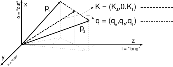
Figure 20: By definition : $Oz$ is chosen along the beam and $\vec{K}$ in the $x-z$ plane. The $L$ (longitudinal) component of a vector is its $z$ component, the $O$ (“outward”) its $x$ component and $S$ (“sidewards”) its $y$ component dessinhbt .

In a first comparison, we used similar initial conditions than above, $T_{0}=200$ MeV (S+S collisions) for both continuous emission and freeze out. Results are presented as function of $q_{L}$,$q_{O}$ and $q_{S}$ in figure 21.

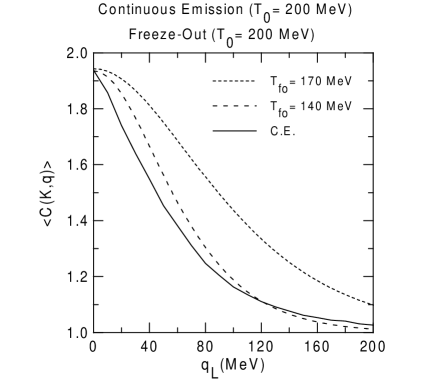
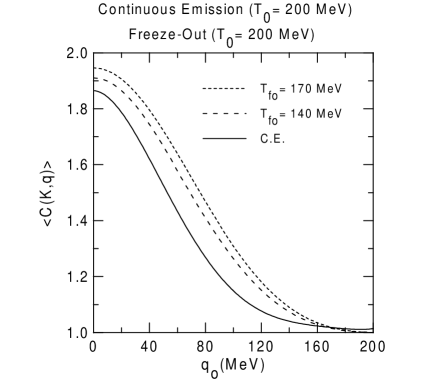
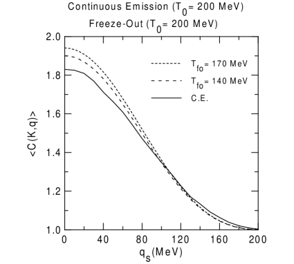
Figure 21: Comparison of continuous emission with freeze out, when both have the same initial conditions Grassi00b .

In a second comparison, given a curve obtained for continuous emission, we try to find a similar curve obtained with the standard value $T_{f.out}=140$ MeV, varying the initial temperature $T^{f.out}_{0}$. The results are shown as function of $q_{L}$,$q_{O}$ e $q_{S}$ in figure 22.

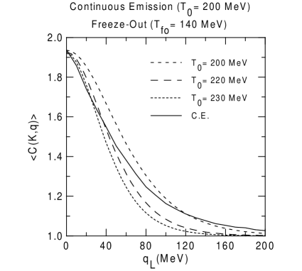
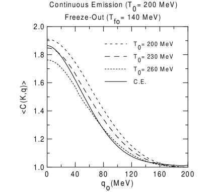
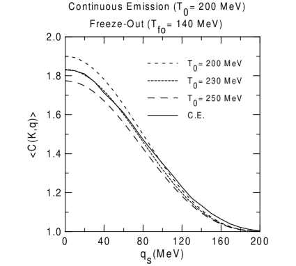
Figure 22: Given a curve obtained for continuous emission, we look for initial conditions for freeze out at $T_{f.out}=140$ MeV leading to a similar curve Grassi00b .

From these two sets of figures, it can be seen that there are many differences in the correlations between both models: shape. heigth, etc. If the initial conditions are the same, the correlations are very different. Even more interesting if trying to approximate with a freeze out at $T_{f.out}=140$ MeV, the continuous emission correlations, it is necessary to assume a $T_{0}$ very high, where the notion of hadronic gas looses its validity. So, we can see that if continuous emission is the correct description for experimental data, it will be more difficult to attain the quark gluon plasma than it looks using the freeze out model. So again we conclude that what we learn about the hot dense matter created depends on the emission model used. ( Note that to actually compare with data, transverse expansion has to be included. )

More recently, we addressed the “HBT puzzle” at RHIC using NeXSPheRIO hbt04 (for a review on NeXSPheRIO, see yogiro_review ). We showed that the use of varying initial conditions leads to smaller radii. In addition, though continuous emission is not easy to introduce in hydrodynamical codes (because (26) depends on the future evolution of the fluid), it was introduced in an approximate way and shown to be important to reproduce the momentum dependence of the radii.

f. Plasma
In all the previous analysis, we assumed that the fluid was initially composed of hadrons with some initial conditions $T_{0}$, $\mu_{b,0}$. Given the possibility that a quark gluon plasma might have been created already, we must discuss the extension of our model to the case were a plasma might have been formed.

Initially, it might be expected that continuous emission by a plasma is impeded for two reasons: 1) a hadron emitted by the plasma surface, in the outward direction, must cross all the hadronic matter around the plasma core , so probably it will suffer collisions and when finally emitted, it will be emitted by the hadronic gas in the way we have considered so far 2) the plasma is formed by colored objects that must recombine in a color singlet at the plasma surface to be emitted, this makes plasma emission more difficult than hadron gas emission.

For simplicity let us consider a second order phase transition. We use for the hadron gas a resonance gas equation of state. For the plasma, we use a MIT bag equation of state where the value of the bag constant and transition temperature are adjusted to get a second order phase transtion. We get $T_{c}\sim 220$ MeV and $B\sim 580$ MeV $fm^{-3}$.

Then we solve the hydrodynamics equation (without continuous emission as a first approximation) to know the localization and evolution of the plasma core. This is shown in figure 23. These equations were also solved for the case of a hadronic gas for comparison in figure 24.

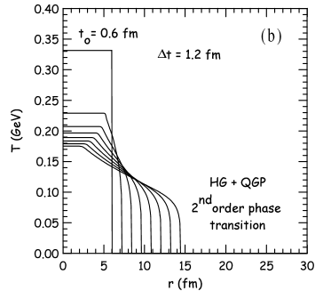
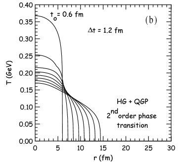
Figure 23: Evolution of temperature in the case of a hadron gas with quark core and initial boxlike matter distribution, top and softer, bottom.

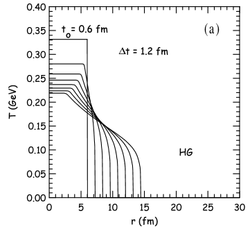
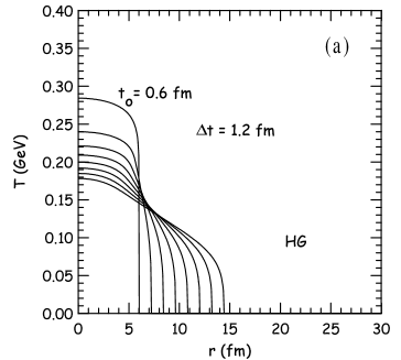
Figure 24: Evolution of temperature in the case of a hadron gas and initial boxlike matter distribution, top and softer, bottom.

It can be checked that when there exists a plasma core, it is quite close to the outside region. Contrarely to the reservation 1) above, hadrons emitted by the plasma surface might be quite close enough to the outside to escape without collisions.

Now for reservation number 2), we note that there exist various mechanisms raf83 ; ban83 ; mu85 ; vi91 ; russe proposed for hadron emission by a plasma. To start we can assume as Visher et al. vi91 that the plasma emits in equilibrium with the hadron gas. In this case, the emission formula by the plasma core+hadron gas would be

$$E\frac{d^{3}N}{dp^{3}} = \int d\phi d\eta[\int_{0}^{\infty}\rho d\rho\left(p^{\tau}f_{free}\tau\right)_{|\tau_{\infty}}$$ (42)

$$+ \int_{\tau_{0}}^{\infty}\tau d\tau\left(p^{\rho}f_{free}\rho\right)_{|R_{out}(\tau)}]$$

where $R_{out}(\tau)$ is the radius up to which there is matter.
This is similar to the hadron gas case treated above. The difference is in the calculation of $\cal P$, (which appears in $f_{free}$), since a hadron entering the plasma core will be supposed detroyed.

In the same spirit as above, a cutoff at ${\cal P}={\cal P_{F}}$ can be introduced. Due to the similarity for the spectra formula with and without plasma core, we do not expect very drastic differences if the transition is second order. Of course, the case of first order transition must be considered (though results from lattice QCD on the lattice do not favour strong first order transition). (Note that $T_{c}\sim 220$ MeV is higher than expected, this might be improved e.g. using a better equation of state).

V Conclusion

In this paper, we discussed particle emission in hydrodynamics. Sudden freeze out is the mechanism commonly used. We described some of its caveats and ways out.

First the problem of negative contributions in the Cooper-Frye formula was presented. When these contributions are neglected, they lead to violations of conservation laws. We showed how to avoid this, the main difficulty remains to compute the distribution function of matter that crossed the freeze out surface. Even models combining hydrodynamics with a cascade code have this type of problem or related ones bu03 .

Assuming that sudden freeze out does hold true, data call for two separate freeze outs. We argue that in this case, this must be included in the hydrodynamical code as it will influence the fluid evolution and the observables. Some works flor using paramatrization of the hydrodynamical solution suggest that a single freeze out might be enough. No hydrodynamical code with simultaneous chemical and thermal freeze outs achieves this so far (see e.g. our figures  9). On the other side, (single) explosive freeze out is being incorporated in a hydrodynamical code csernaicode .

Finally, we argued that microscopical models indeed do not indicate a sudden freeze out but a continuous emission Bra ; Sor ; Bas . We showed how to formulate particle emission in hydrodynamics for this case and discussed extensively its consistency with data. We pointed out in various cases that the interpretation of data is quite influenced by the choice of the particle emission mechanisms. The formalism that we presented for continuous emission needs improvements, for example the ansatz of immediate rethermalization is not realistic. An example of such an attempt is yogiro . Finally, it is also necessary to think of ways to include continuous emission in hydrodynamics. This is not trivial because the probability to escape depends on the future. In hbt04 , such an idea was applied to the “HBT puzzle” at RHIC with promising results.

V.1 Acknowledgments

This work was partially supported by FAPESP (2000/04422-7). The author wishes to thank L.Csernai and S.Padula for reading parts of the manuscript prior to submission.

References

- (1) “Collected papers of L.D.Landau” p. 665, ed. D.Ter-Haar, Pargamon, Oxford, 1965.
- (2) E.Fermi Prog. Theor. Phys. 5 (1950) 570
- (3) Y.Hama, T.Kodama & S.Paiva Phys. Rev. C55 (1997) 1455; Found. of Phys. 27 (1997) 1601.
- (4) C.Aguiar, Y.Hama, T.Kodama & T.Osada Nucl. Phys. A698 (2002) 639c.
- (5) Y.Hama & F.Pottag Rev. Bras. Fis. 15 (1985) 289.
- (6) T.Csörgo, F.Grassi, Y.Hama & T.Kodama Phys. Lett. B565 (2003) 107-115
- (7) H.-T. Elze, Y.Hama, T.Kodama, M.Markler & J.Rafelski J. Phys. G25 (1999) 1935
- (8) C.Aguiar, T.Kodama, T.Osada & Y.Hama J. Phys. G27 (2001) 75; Nucl. Phys.A698 (2002) 639c.
- (9) D.Menezes, F.Navarra, M.Nielsen & U.Ornik Phys. rev. C47 (1993) 2635
- (10) C.Aguiar & T.Kodama Phys. A320 (2003) 371
- (11) Y.Hama & S.Padula Phys. Rev. D37 (1988) 3237
- (12) S.Padula & C.Roldão Phys. Rev. C58 (1998) 2907
- (13) S.Padula Nucl. Phys. A715 (2002) 637c
- (14) F.Grassi, Y.Hama, S.Padula & O.Socolowski Jr. Phys. Rev. C62 (2000) 044904
- (15) F.Grassi & O.Socolowski Jr. Phys. Rev. Lett. 80 (1998) 1770
- (16) F.Grassi & O.Socolowski Jr. J. Phys. G25 (1999) 331
- (17) F.Grassi & O.Socolowski Jr. J. Phys. G25 (1999) 339
- (18) Y.Hama & F.Navarra Z.Phys. C53 (1991) 501
- (19) F.Navarra, M.C.Nemes, U.Ornik & S.Paiva Phys. Rev. C45 (1992) R2552
- (20) F.Grassi, Y.Hama & T.Kodama Phys. Lett. B355 (1995) 9; Z.Phys. C73 (1996) 153.
- (21) V.K.Margas, Cs.Anderlik, L.P.Csernai, F.Grassi, W.Greiner, Y.Hama, T.Kodama, Zs.I.Lázár & H.Stöcker Phys. Lett. B459 (1999) 33; Phys. Rev. C59 (1999) 3309; Nucl. Phys. A661 (1999) 596.
- (22) N.Arbex, F.Grassi, Y.Hama & O.Socolowski Jr. Phys. Rev. C64 (2001) 064906
- (23) Yu.M.Sinyukov, S.V.Akkelin and Y.Hama Phys.Rev.Lett. 89 (2002) 052301
- (24) T.Hirano Phys.Rev.Lett. 86 (2001) 2754; Phys.Rev. C65 (2002) 011901; T.Hirano, K.Morita, S.Muroya and C.Nonaka Phys.Rev. C65 (2002) 061902; T.Hirano and K.Tsuda Phys.Rev. C66 (2002) 054905
- (25) U.Heinz,K.S.Lee and M.Rhoades-Brown, Phys.Rev.Lett. 58 (1987) 2292.
- (26) K.S.Lee, M.Rhoades-Brown and U.Heinz,, Phys. Rev. C37 (1988) 1463.
- (27) C.M.Hung and E.Shuryak, Phys. Rev. C57 (1998) 1891.
- (28) K.S. Lee, U. Heinz, and E. Schnerdermann, Z.Phys.C 48(1990)525
- (29) F. Cooper and G. Frye, Phys.Rev. D10 (1974) 186.
- (30) L.Bravina et al. Phys. Lett. B354 (1995) 196. Phys. Rev.C60 (1999)044905.
- (31) H. Sorge, Phys. Lett. B373 (1996) 16.
- (32) S.Bass et al. Phys. Rev. C69(1999)021902
- (33) S. Bernard et al., Nucl. Phys. A605 (1996) 566.
- (34) D.H. Rischke, Proceedings of the 11th Chris Engelbrecht Summer School in Theoretical Physics, Cape Town, February 4-13, 1998, nucl-th/9809044.
- (35) Cs. Anderlik, Zs.I.Lázár,V.K.Margas, L.P.Csernai, W.Greiner, & H.Stöcker Phys.Rev. C59 (1999) 388
- (36) V.K.Margas,Cs. Anderlik,L.P.Csernai, F.Grassi, W.Greiner, Y.Hama,T.Kodama, Zs.I.Lázár & H.Stöcker Heavy Ion Phys. 9 (1999) 193
- (37) K.Tamosiunas and L.P.Csernai, Eur. Phys. J. A20 (2004) 269.
- (38) L.P.Csernai, V.K.Margas, E.Molnar, A. Nyiri and K.Tamosiunas hep-ph/0406082
- (39) V.K.Margas,A.Anderlik, Cs.Anderlik, L.P.Csernai Eur.Phys.J. C30 (2003) 255
- (40) D.Teanay et al. Phys. Rev. Lett. 86 (2001) .
- (41) S.Bass and A.Dumitru Phys. Rev. C61 (2000) 064909.
- (42) K.A. Bugaev Phys. Rev. Lett. 90 (2003) 252301.
- (43) C.Slotta, J.Sollfrank and U.Heinz, Proceedings of Strangeness in Quark Matter ’95, AIP Pess, Woobury, NY.
- (44) K.Redlich et al.NPA556(1994)391.
- (45) J.Sollfrank, J.Phys. G23 (1997) 1903.
- (46) Davidson,N.J. et al. Phys. Lett. B255(1991)105
- (47) J.Sollfrank et al. Z.Phys. C61 (1994) 659.
- (48) V.K.Tawai et al. Phys. Rev. C53 (1996) 2388.
- (49) A.D.Panagiotou et al. Phys. Rev. C53 (1996) 1353.
- (50) F.Becattini, J.Phys. G23 (1997) 287.
- (51) J.Sollfrank, próprios resultados.
- (52) G.Andersen et al., Phys. Lett. B327 (1994) 433.
- (53) J.Letessier et al., Phys. Rev. D51 (1995) 3408.
- (54) P.Braun-Munzinger et al. Phys. Lett. B365 (1996) 1.
- (55) C.Spieles et al., Eur.Phys.J. C2 (1998) 351.
- (56) N.Xu et al., NA44 collaboration, Nucl. Phys. A610 (1996) 175c.
- (57) U.E.Wiedermann, B.Tomásik and U.Heinz, Nucl. Phys. A638 (1997) 475c.
- (58) U.Heinz Nucl. Phys. A638 (1998) 357c.
- (59) J.D.Bjorken, Phys. Rev. D27 (1983) 140.
- (60) N. Arbex, U. Ornik, M. Plümer and R. Weiner, Phys.Rev. C55 (1997) 860.
- (61) D.Teaney nucl-th/0204023.
- (62) F.Grassi, Y.Hama and T.Kodama, Phys. Lett. B355(1995)9
- (63) F.Grassi,Y.Hama and T.Kodama, Z. Phys. C73(1996)153
- (64) F. Grassi and O.Socolowski Jr., Heavy Ion Phys. 4(1996)257.
- (65) F.Grassi, Y.Hama, T.Kodama & O.Socolowski Jr., Heavy Ion Phys. 5 (1997) 417.
- (66) F.Grassi and O.Socolowski, Phys. Rev. Lett.80 (1998) 1170.
- (67) F.Grassi and O.Socolowski, J.Phys.G 25 (1999) 331.
- (68) F.Grassi & O.Socolowski, J.Phys.G 25 (1999) 339.
- (69) Van Hecke et al. Phys. Rev. Lett.81(1998)5764.
- (70) S.Bass et al., Prog.Part.Nucl.Phys. 41 (1998) 225.
- (71) L.Bravina et al. , J.Phys. G25 (1999) 351.
- (72) O.Socolowski Jr., Ph.D. thesis, april 99, IFT-UNESP.
- (73) L.S̆ándor et al. (WA97) J. Phys. G30 (2004) S129.
- (74) M. van Leeuwen et al. (NA49) Nucl. Phys. A715 (2003) 161c.
- (75) U. Heinz J. Phys. G30 (2004) S251.
- (76) J. Castillo et al. (STAR) J. Phys. G30 (2004) S181.
- (77) C.Alt et al. nucl-ex/0409004
- (78) F.Antinori et al. J.Phys.G30 (2004) 823.
- (79) F.Grassi,Y.Hama, T.Kodama and O.Socolowski Jr., Proceedings of Strangeness in Quark Matter 2004, a parecer em J.Phys.G.
- (80) N.J.Davidson et al. Z. Phys. C56(1992)319.
- (81) J.Cleymans et al. Z.Phys.C58 (1993) 347.
- (82) Ster et al., Nucl. Phys. A661(1999)419c.
- (83) Tomásik et al., Heavy Ion Phys. 17 (2003) 105.
- (84) R.A.Ritchie et al.,Phys. Rev. C75(1997) 535.
- (85) G.D.Yen et al., Phys. Rev. C56 (1997) 2210.
- (86) G.D.Yen and M.Gorenstein, Phys.Rev. C59 (1999) 2788.
- (87) J.Letessier et al., Phys. Rev. Lett. 70 (1993) 3530.
- (88) J.Letessier et al., Phys. Rev. C59 (1999) 947.
- (89) F.Grassi, Y. Hama, T. Kodama and O.Socolowski Jr., J.Phys.G.30 (2004) 853
- (90) S.Padula, these Proceedings.
- (91) F.Grassi, Y. Hama, S.Padula and O.Socolowski Jr., Phys. Rev. C62 (2000) 044904.
- (92) K.Kolehmainen and M.Gyulassy, Phys. Lett. B189 (1986) 203.
- (93) U.A.Wiedemann and U.Heinz, Phys.Rept. 319 (1999) 145
- (94) O. Socolowski Jr., F. Grassi, Y. Hama and T. Kodama, Phys.Rev.Lett.93 (2004)182301.
- (95) Y. Hama, T. Kodama and O. Socolowski Jr., these Proceedings.
- (96) M.Danos & J.Rafelski, Phys. Rev. D27 (1983) 671
- (97) B.Banerjee, N.K.Glendening & T.Matsui, Phys. Lett. B127 (1983) 453.
- (98) B.Müller & J.M.Eisenberg, Nucl. Phys. A 435 (1985) 791
- (99) A.Visher et al. Phys. Rev. D43 (1991) 271.
- (100) D.Yu.Peressunko & Yu.E.Pokrovsky Nucl. Phys. A624 (1997)738; hep-ph/0002068v2
- (101) W.Broniowski and W.Florkowski Phys.Rev. C65 (2002) 064905; AIP Conf.Proc. 660 (2003) 177. W.Broniowski, A.Baran and W.Florkowski AIP Conf.Proc. 660 (2003) 185.
- (102) L.P. Csernai et al. hep-ph/0401005.