The Modified J-Matrix Approach for Cluster Descriptions of Light Nuclei

Abstract

We present a fully microscopic three-cluster nuclear model for light nuclei on the basis of a J-Matrix approach. We apply the Modified J-Matrix method on ${}^{6}He$ and ${}^{6}Be$ for both scattering and reaction problems, analyse the Modified J-Matrix calculation, and compare the results to experimental data.

1 Introduction

The J-Matrix method (JM) has proven very successful in microscopic nuclear calculations, particularly the Modified J-Matrix approach (MJM)[1, 2], also called the Algebraic Model in some nuclear physics literature. Both collective [3] and cluster descriptions [4, 5], of light (p-shell) nuclei have been studied with the MJM, using an oscillator basis.

The Harmonic Oscillator basis has always been very popular in nuclear physics. For light nuclei, spherical oscillator states have often been used as a first approximation to the single-particle orbital wave functions in the popular nuclear shell-model. The nuclear many-body basis is then built up as a set of Slater determinants of single-particle oscillator orbital states to take the Pauli principle into account.

Many nuclear two-body potentials feature a superposition of Gaussian components. Matrix elements of two-body operators for Slater determinants reduce to a simple sum of two-body matrix elements, involving the single-particle oscillator states. A Gaussian form of the operator then easily leads to an analytical form for the matrix elements. This immediately shows the computational advantage of using an oscillator state (or even a superposition of oscillator states) for the single-particle wave functions in a fully microscopic many-body nuclear model.

One of the features of the oscillator basis is the Jacobi (tridiagonal) form of the matrix of the kinetic energy operator. This makes it a proper candidate for considering the JM approach to solve the Schrödinger equation expressed in matrix form.

The nuclear many-body system is very complex though, and requires huge superpositions of shell-model states to reproduce spectral properties over an important energy range. Also, the nuclear system exhibits several modes when the system is energetically excited, and possibly fragmented. There is an interplay between collective modes, such as monopole and quadrupole excitations, and cluster effects that are particularly pronounced when the nucleus disintegrates. One therefore often introduces very specific antisymmetrized forms for the wave function with a specific configuration of single-particle orbitals, that feature some specific collective behavior that one wants to study. In this way the Hilbert space is limited to a single (or a few coupled) nuclear model state(s) in which the collective coordinates are the only remaining dynamical coordinates. The dimensions of the Schrödinger equation are then strongly reduced.

Although the nuclear two-body interaction has a short range, the effective interaction as a function of the collective coordinates often displays a long range. If the collective behavior is described as a superposition of oscillator states, this is usually also reflected in the matrix elements of the nuclear potential, which display a slow decrease for increasing oscillator excitation. This clearly limits the applicability of the standard JM method, as too large energy matrices have to be considered in the internal, non-asymptotic, region. Indeed, the main computational cost for nuclear JM calculations often lies in the construction of the matrix elements of highly excited states. To account for this limitation the MJM approach was developed [1, 2], introducing a semi-classical approximation for the matrix elements in the highly excited internal region. This leads to a modification of the standard three-term recursion relation for the far interaction and asymptotic region by including (semiclassical) potential contributions. A drastic reduction of the matching position for boundary condition is obtained, resulting in a remaining matrix equation of manageable dimensions.

The Coulomb contribution to the nuclear potential, which is known to have a long range, can be handled in the same way.

In the following sections we will elaborate on the cluster description of nuclei as an important collective description for the lightest nuclei, in which the internuclear distances then become the dynamical (collective) coordinates. We will link this model to the MJM approach to solve the Schrödinger equation, and present applications on 6-particle nuclear systems where three-cluster effects are important. We will compare the theoretical results to the experimental ones to test the validity of the approach.

2 JM Cluster models for light nuclei

Two- and three-cluster configurations carry an important part of the low-energy physics in light nuclei, and directly relate to scattering and reaction experiments in which smaller fragments are used to study compound properties.

In this section we discuss the three-cluster description for light nuclei. Where appropriate we briefly present some two-cluster properties, as the three-cluster approach is essentially a generalization hereof.

The many-particle wave functions for a three-cluster system of $A$ nucleons ($A=A_{1}+A_{2}+A_{3}$) can be written, using the anti-symmetrization operator $\mathcal{A}$, as follows

$$\Psi\left(\mathbf{q}_{1},..,\mathbf{q}_{A-1}\right)=\mathcal{A}\left[\Psi_{1}\left(A_{1}\right)\ \Psi_{2}\left(A_{2}\right)\ \Psi_{3}\left(A_{3}\right)\ \Psi_{R}\left(R\right)\right]$$ (1)

where the centre of mass of the $A$-nucleon system has been eliminated by the use of Jacobi coordinates $\mathbf{q}_{i}$ so that only internal dynamics are described. The cluster wave functions $\Psi_{i}\left(A_{i}\right)$

$$\Psi_{i}\left(A_{i}\right)=\Psi_{i}\left(\mathbf{q}_{1}^{\left(i\right)},..,\mathbf{q}_{A_{i}-1}^{\left(i\right)}\right)\quad(i=1,2,3)$$ (2)

represent the internal structure of the $i$-th cluster, centered around its centre of mass $\mathbf{R}_{i}$. To limit the computational complexity of the problem, these cluster functions are fixed and they are Slater determinants of harmonic oscillator ($0s$)-states, corresponding to the groundstate shell-model configuration of the cluster ($A_{i}\leq 4$ for all $i$). The $\Psi_{R}\left(R\right)$ wave function

$$\Psi_{R}\left(R\right)=\Psi_{R}\left(\mathbf{q}_{1}^{\left(R\right)},\mathbf{q}_{2}^{\left(R\right)}\right)=\Psi_{R}\left(\mathbf{q}_{1},\mathbf{q}_{2}\right)$$ (3)

represents the relative motion of the three clusters with respect to one another, and $\mathbf{q}_{1}$ and $\mathbf{q}_{2}$ represent Jacobi coordinates. In figure 1 we indicate an enumeration of possible Jacobi coordinates and their relation to the component clusters.

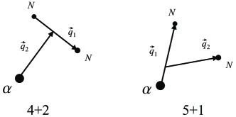
Figure 1: Two configurations of Jacobi coordinates for the three-cluster system $\alpha+N+N$.

The state (3) is not limited to any particular type of orbital; on the contrary we will use a complete basis of harmonic oscillator states for the relative motion degrees of freedom. Thus the full $A$-particle state cannot be expressed as a single Slater determinant of single particle orbitals.

An important approximation, known as the “Folding” model, is obtained by breaking the Pauli principle between the individual clusters, but retaining a proper quantum-mechanical description of the clusters, which is described by the wave function

$$\Psi_{F}\left(\mathbf{q}_{1},..,\mathbf{q}_{A-1}\right)=\Psi_{1}\left(A_{1}\right)\ \Psi_{2}\left(A_{2}\right)\ \Psi_{3}\left(A_{3}\right)\ \Psi_{R}\left(R\right)$$ (4)

Because each cluster wave function is antisymmetric (they are Slater determinants) one is indeed neglecting the inter-cluster anti-symmetrization only. The Folding Model has the advantage of preserving the identities of the clusters and, if the intra-cluster structure is kept “frozen”, it reduces the many-particle problem to that of the relative motion of the clusters.

For a two-cluster description the formulae simplify to:

$$\Psi\left(\mathbf{q}_{1},..,\mathbf{q}_{A-1}\right)=\mathcal{A}\left[\Psi_{1}\left(A_{1}\right)\ \Psi_{2}\left(A_{2}\right)\ \Psi_{R}\left(R\right)\right]$$ (5)

with

$$\Psi_{R}\left(R\right)=\Psi_{R}\left(\mathbf{q}_{0}^{\left(R\right)}\right)=\Psi_{R}\left(\mathbf{q}_{0}\right)$$ (6)

The folding approximation will be the natural choice for calculating the asymptotic behavior of the cluster-system, i.e. the disintegration of the system in the two or three non-interacting individual clusters. This amounts to the situation that all clusters are a sufficient distance apart and inter-cluster antisymmetrization has a negligible effect.

Because the cluster states are fixed and built up of ($0s$)-orbitals, the problem of labeling the basis states with quantum numbers relates to the inter-cluster wave function only. This holds true whether one uses the full anti-symmetrization or the folding approximation. In a two-cluster case, the set of quantum numbers describing inter-cluster motion is unambiguously defined, and is obtained from the reduction of the symmetry group $U(3)\supset O(3)$ of the one-dimensional oscillator. This reduction provides the quantum numbers $n$ for the radial excitation, and $L,M$ for the angular momentum of the two-cluster system.

In a three-cluster case, several schemes can be used to classify the inter-cluster wave function in the oscillator representation. In [6, 7] three distinct but equivalent schemes were considered. One of these used the quantum numbers provided by the Hyperspherical Harmonics (HH) method (see for instance [8, 9, 10]). This is the classification that we will adopt. Even within this particular scheme there are several ways to classify the basis states. We shall restrict ourselves to the so-called Zernike-Brinkman basis [11]. This corresponds to the following reduction of the unitary group $U(6)$, the symmetry group of the three-particle oscillator Hamiltonian,

$$U(6)\supset O(6)\supset O(3)\otimes O(3)\supset O(3)$$ (7)

This reduction provides the quantum numbers $K$, the hypermomentum, $n$, the hyperradial excitation, $l_{1}$, the angular momentum connected with the first Jacobi vector, $l_{2}$, the angular momentum connected with the second Jacobi vector, and $L$ and $M$ the total angular momentum obtained from coupling the partial angular momenta $l_{1}$, $l_{2}$. Collectively these quantum numbers will be denoted by $\nu$, i.e. $\nu=\{n,K,(l_{1}l_{2})LM\}$ in the remainder of the text.

There are a number of relations and constraints on these quantum numbers:

• the total angular momentum is the vector sum of the partial angular momenta $\mathbf{l}_{1}$and $\mathbf{l}_{2}$, i.e. $\mathbf{L}=$ $\mathbf{l}_{1}+$ $\mathbf{l}_{2}$ or $\left|l_{1}-l_{2}\right|\leq L\leq l_{1}+l_{2}$.

• by fixing the values of $l_{1}$ and $l_{2}$, we impose restrictions on the hypermomentum $K=l_{1}+l_{2},~{}l_{1}+l_{2}+2,~{}l_{1}+l_{2}+4,\ldots$ This condition implies that for certain values of hypermomentum $K$ the sum of partial angular momenta $l_{1}+l_{2}$ cannot exceed $K$.

• the partial angular momenta $l_{1}$ and $l_{2}$ define the parity of the three-cluster state by the relation $\pi=\left(-1\right)^{l_{1}+l_{2}}$.

• for the “normal” parity states $\pi=\left(-1\right)^{L}$ the minimal value of hypermomentum is $K_{\min}=L$, whereas $K_{\min}=L+1$ for the so-called “abnormal” parity states $\pi=\left(-1\right)^{L+1}$.

• oscillator shells with $N$ quanta are characterized by the constraint $N=2n\;+K$.

Thus for a given hyperangular and rotational configuration the quantumnumber $n$ ladders the oscillator shells of increasing oscillator energy.

2.1 Asymptotic solutions in coordinate representation

The MJM method for solving the Schrödinger equation for quantum scattering systems is based on a matrix representation of the Schrödinger equation in terms of a square integrable basis. In a nuclear context the Harmonic Oscillator basis is appropriate. The boundary conditions are ultimately formulated in terms of the asymptotic behavior of the expansion coefficients of the wave function.

In the case of three-cluster calculations, one needs to determine the asymptotic behavior of the wave function. Consider an expansion of the relative wave function

$$\Psi_{R}\left(\mathbf{q}_{1},\mathbf{q}_{2}\right)=\sum_{\nu}c_{\nu}\Psi_{\nu}\left(\mathbf{q}_{1},\mathbf{q}_{2}\right)$$ (8)

with $\nu=\{n,K,(l_{1}l_{2})LM\}$ and $\left\{\Psi_{\nu}\right\}$ a complete basis of six-dimensional oscillator states. It covers all possible types of relative motion between the three clusters.

To obtain the asymptotic behavior of the three-cluster system the folding approximation is used. The assumption that antisymmetrization effects between clusters are absent in the asymptotic region is a natural one. It simplifies the many-body dynamics effectively to that of a three-particle system, as the cluster descriptions are frozen. The relative motion problem of the three clusters in the absence of a potential (i.e. considering the JM reference Hamiltonian only) can then be explicitly solved in the HH method (see for instance [8, 9, 10]). It involves the transformation of the Jacobi coordinates $\mathbf{q}_{1}$ and $\mathbf{q}_{2}$ to the hyperradius $\rho$ and a set of hyperangles $\Omega$. The hyperspherical coordinates $\rho$ and $\Omega$ describe the geometry of the three-particle system in the same way that the spherical coordinates describe the geometry of two-particle systems. The inter-cluster wave function in coordinate representation is expanded in HH’s $H_{K}^{\nu_{0}}\left(\Omega\right)$ where $\nu_{0}$ has been chosen as a shorthand for $(l_{1}l_{2})LM$, and which are the generalization of the spherical harmonics $Y_{LM}\left(\theta,\varphi\right)$.

In the absence of the Coulomb interaction this leads to a set of equations for the hyperradial asymptotic solutions, with the kinetic energy operator as the JM reference Hamiltonian

$$\left\{-\frac{\hbar^{2}}{2m}\left[\frac{d^{2}}{d\rho^{2}}+\frac{5}{\rho}\frac{d}{d\rho}-\frac{K\left(K+4\right)}{\rho^{2}}\right]-E\right\}R_{K,\nu_{0}}\left(\rho\right)=0$$ (9)

The solutions can be obtained analytically and are represented by a pair of Hänkel functions for the ingoing and outgoing solutions:

$$R_{K,\nu_{0}}^{\left(\pm\right)}\left(\rho\right)=\left\{\begin{array}[c]{l}H_{K+2}^{\left(1\right)}\left(k\rho\right)/\rho^{2}\\ H_{K+2}^{\left(2\right)}\left(k\rho\right)/\rho^{2}\end{array}\right\}$$ (10)

where

$$k=\sqrt{\frac{2mE}{\hbar^{2}}}$$

One notices that these asymptotic solutions are independent of all quantum numbers $\nu_{0}$, and are determined by the value of hypermomentum $K$ only. In particular, different $K$-channels are uncoupled.

When charged clusters are considered the asymptotic reference Hamiltonian should consist of the kinetic energy and the Coulomb interaction:

$$\left\{-\frac{\hbar^{2}}{2m}\left[\frac{d^{2}}{d\rho^{2}}+\frac{5}{\rho}\frac{d}{d\rho}-\frac{\left\|\mathcal{K}\right\|}{\rho^{2}}\right]+\frac{\left\|Z_{eff}\right\|}{\rho}-E\right\}\left\|\mathcal{R}\left(\rho\right)\right\|=0$$ (11)

The matrix $\left\|\mathcal{K}\right\|$ is diagonal with matrix elements $K\left(K+4\right)$, and $\left\|Z_{eff}\right\|$, the “effective charge”, is off-diagonal in $K$ and $(l_{1}l_{2})$. The solution matrix $\left\|\mathcal{R}\left(\rho\right)\right\|$ reflects the coupling of $K$-channels. A standard approximation for solving these equations is to decouple the $K$-channels, by assuming that the off-diagonal matrix-elements of $\left\|Z_{eff}\right\|$ are sufficiently small:

$$\left\{-\frac{\hbar^{2}}{2m}\left[\frac{d^{2}}{d\rho^{2}}+\frac{5}{\rho}\frac{d}{d\rho}-\frac{K\left(K+4\right)}{\rho^{2}}\right]+\frac{Z_{eff}}{\rho}-E\right\}R_{K,\nu_{0}}\left(\rho\right)=0$$ (12)

The constants $Z_{eff}$ depends on $K$ and $\nu_{0}$ and all parameters of the many-body system under consideration. We will restrict ourselves to this decoupling approximation, but it is to be understood that its validity has to be checked for any specific three-cluster system.

The asymptotic solutions then become

$$R_{K,\nu_{0}}^{\left(\pm\right)}\left(\rho\right)=\frac{1}{\sqrt{k}}W_{\pm i\eta,K+2}\left(\pm 2ik\rho\right)/\rho^{\frac{5}{2}}$$ (13)

where $W$ is the Whittaker function and $\eta$ is the well-known Sommerfeld parameter

$$\eta=\frac{m}{2\hbar^{2}}\frac{Z_{eff}}{k}$$ (14)

As $\eta$ is a function of $K,$ $l_{1}$ and $l_{2}$ through the parameter $Z_{eff}$, the asymptotic solutions will now be dependent on $K$ and $\nu_{0}$.

A two-cluster description leads to the well-known one-dimensional radial equation, with asymptotic solutions

$$R_{L}^{\left(\pm\right)}\left(\rho\right)=\frac{1}{\sqrt{k}}W_{\pm i\eta,L+\frac{1}{2}}\left(\pm 2ik\rho\right)/\rho$$

where $\rho$ now is the inter-cluster radial distance and $\eta$ is the Sommerfeld parameter with $Z_{eff}=Z_{1}Z_{2}e^{2}\sqrt{\frac{A_{1}A_{2}}{A_{1}+A_{2}}}$

One can easily combine the two- and three cluster asymptotics in a single representation as

$$R_{\mathcal{L}}^{\left(\pm\right)}\left(\rho\right)=\frac{1}{\sqrt{k}}W_{\pm i\eta,\lambda}\left(\pm 2ik\rho\right)/\rho^{\frac{\sigma-1}{2}}$$ (15)

where the parameters $\mathcal{L}$, $\lambda$, $\sigma$ and $\eta$, differ for the two- and three-cluster channels, and are summarized in Table 2.

Table 1: Two- and three-cluster asymptotic solution parameters

	$\mathcal{L}$	$\sigma$	$\lambda$	$\eta$
two-cl. channel	$L$	3	$L+\frac{1}{2}$	$\frac{Z_{1}Z_{2}e^{2}}{k}\frac{m}{2\hbar^{2}}\sqrt{\frac{A_{1}A_{2}}{A_{1}+A_{2}}}$
three-cl. channel	$K$	6	$K+2$	$\frac{Z_{eff}}{k}\frac{m}{2\hbar^{2}}$

2.2 Asymptotic solutions in oscillator representation

The JM relies on an expansion in terms of oscillator functions, and the asymptotic behavior of the corresponding expansion coefficients $c_{\nu}$. We will restrict ourselves to the three-cluster situation; the two-cluster results can be readily obtained from [2] and the results of the section 2.1.

It was conjectured (see for instance [2]) that for very large values of the oscillator quantum number $n$ the expansion coefficients for physically relevant wave-functions behave like

$$c_{n}=\left\langle n|\psi\right\rangle\simeq\sqrt{2}\rho_{n}^{2}\psi(b\rho_{n})$$ (16)

with $b$ the oscillator parameter of the basis, $\rho_{n}=\sqrt{4n+2K+6}$ the classical turning point, and $\psi$ the hyperradial wave function.

In the case of neutral clusters this leads after substitution of the hyperradial asymptotic solutions to the following expansion coefficients $c_{n}^{\left(\pm\right)}$

$$c_{n}^{\left(\pm\right)K}\simeq\sqrt{2}\left\{\begin{array}[c]{l}H_{K+2}^{\left(1\right)}\left(kb\rho_{n}\right)\\ H_{K+2}^{\left(2\right)}\left(kb\rho_{n}\right)\end{array}\right\}$$ (17)

This result can be obtained in an alternative way [12, 13] by representing the Schrödinger equation, with the kinetic energy operator $\hat{T}$ as the reference Hamiltonian to describe the asymptotic situation, in a (hyperradial) oscillator representation

$$\sum_{m=0}^{\infty}\left\langle n,\left(K,\nu_{0}\right)\left|\hat{T}-E\right|m,\left(K,\nu_{0}\right)\right\rangle c_{m}^{K,\nu_{0}}=0$$ (18)

This matrix equation is of a three-diagonal form because of the properties of $\hat{T}$ and the oscillator basis. Solving for the expansion coefficients $c_{n}^{K,\nu_{0}}$ leads to a three-term recurrence relation

$$T_{n,n-1}^{K,\nu_{0}}c_{n-1}^{K,\nu_{0}}+\left(T_{n,n}^{K,\nu_{0}}-E\right)c_{n}^{K,\nu_{0}}+T_{n,n+1}^{K,\nu_{0}}c_{n+1}^{K,\nu_{0}}=0$$ (19)

where

$$T_{n,m}^{K,\nu_{0}}=\left\langle n,\left(K,\nu_{0}\right)\left|\hat{T}\right|m,\left(K,\nu_{0}\right)\right\rangle$$ (20)

The asymptotic solutions (i.e. for high $n$) of this recurrence relation are then precisely given by (17).

When the Coulomb interaction is present we again apply (16) to obtain

$$c_{n}^{\left(\pm\right)K}\simeq\sqrt{2}\left\{\begin{array}[c]{l}W_{i\eta,\mu}\left(2ikb\rho_{n}\right)/\sqrt{\rho_{n}}\\ W_{-i\eta,\mu}\left(-2ikb\rho_{n}\right)/\sqrt{\rho_{n}}\end{array}\right\}$$ (21)

In this case the oscillator representation of the Schrödinger equation is no longer of a tridiagonal form, and cannot be solved analytically for the asymptotic solutions to corroborate this result.

It should be noted that the above elaborations are valid for relatively small values of momentum $k$ to which correspond sufficiently large values of the discrete hyperradius $\rho_{n}$, which defines the asymptotic region. So for any value of $k$ one can determine a minimum value for $n$ to be safely in the asymptotic region.

As we consider an asymptotic decoupling in the $\left(K,\nu_{0}\right)$ quantumnumbers, one will deal with asymptotic channels characterized by the $\left(K,\nu_{0}\right)$ values. So only in the internal (or interaction) region will states with different $K$ and $\nu_{0}$ be coupled by the short-range nuclear potential and the Coulomb potential. The three-cluster system can therefore be described by a coupled-channels approach, where the individual channels are characterized by a single $K$-value, and we will henceforth refer to these channels as “$K$-channels”.

2.3 Multi-channel JM equations

In the current many-channel description of the JM formulation for three-cluster systems, the channels will be characterized by the a specific value of the set of quantumnumbers $K,\nu_{0}$, whereas the relative motion of clusters within the channel is connected to the oscillator index $n$. We will use $K$ henceforth as an aggregate index for individual channels, and assume it represents all $K,\nu_{0}$ quantum numbers.

The Schrödinger equation can be cast in a matrix equation of the form

$$\sum_{K^{\prime},m}\left\langle n,K\left|\hat{H}-E\right|m,K^{\prime}\right\rangle\ c_{m}^{K^{\prime}}=0$$ (22)

As we will consider an $S$-matrix formulation of the scattering problem, the expansion coefficients are rewritten as

$$c_{n}^{K}=c_{n}^{(0)K}+\delta_{K_{i}K}c_{n}^{(-)K}-S_{K_{i}K}c_{n}^{(+)K}$$ (23)

where, for each channel $K$, the $c_{n}^{(0)K}$ are the so-called residual coefficients, the $c_{n}^{(\pm)K}$ are the incoming and outgoing asymptotic coefficients. The matrix element $S_{K_{i}K}$ describes the coupling between the current channel $K$ and the entrance channel $K_{i}$.

As shown in [14, 15, 16], the $c_{n}^{(\pm)K}$ satisfy the following system of equations

$$\sum_{m=0}^{\infty}\left\langle n,K\left|\hat{H}_{0}-E\right|m,K\right\rangle\ c_{m}^{(\pm)K}=\beta_{0}^{(\pm)K}\ \delta_{n,0}$$ (24)

$\hat{H}_{0}$ being the asymptotic reference Hamiltonian, consisting of the kinetic energy operator for uncharged clusters, and the kinetic energy operator plus Coulomb interaction for charged clusters. The right-hand side for the equation for $c_{m}^{(-)K}$ features $\beta_{0}^{(-)K}$ which is a regularization factor to account for the irregular behavior of the $c_{0}^{(-)K}$. This factor allows one to solve (24) for all values of $n$. The value of $\beta_{0}^{(-)K}$ can be obtained for both reference Hamiltonians (i.e. with or without Coulomb). We introduced $\beta_{0}^{(+)K}=0$ to keep the equations in a homogeneous form.

The set of equations (24) for the asymptotic coefficients can then be solved numerically to different degrees of approximation depending on the requested precision. The $c_{n}^{\left(\pm\right)K\text{ }}$have the desired asymptotic behavior (cfr eqs 17 and 21).

Substitution of (23) in the equations (22) then leads to the following system of dynamical equations for the many-channel system:

$$\sum_{K^{\prime},m}\left\langle n,K\left|\hat{H}-E\right|m,K^{\prime}\right\rangle c_{m}^{\left(0\right)K^{\prime}}-\sum_{K^{\prime}}S_{K_{i}K^{\prime}}V_{n}^{\left(+\right)KK^{\prime}}=-\beta_{0}^{(-)K}\ \delta_{n,0}\delta_{K_{i}K}-V_{n}^{\left(-\right)KK_{i}}$$ (25)

where the coefficients $V_{n}^{\left(\pm\right)KK^{\prime}}$, defined in [2], are given by

$$V_{n}^{(\pm)KK^{\prime}}=\sum_{m=0}^{\infty}\left\langle n,K\left|\hat{V}\right|m,K^{\prime}\right\rangle\ c_{m}^{(\pm)K^{\prime}}$$ (26)

This system of equations should be solved for both the residual coefficients $c_{n}^{\left(0\right)K}$ and the $S$-matrix elements $S_{K^{\prime}K}$.

To obtain an appropriate approximation to the exact solution of (25), we consider an internal region corresponding to $n<N$ and an asymptotic region with $n\geq N$. The choice of $N$ is such that one can expect the residual expansion coefficients $\left\{c_{n}^{(0)K}\right\}$ to be sufficiently small in the asymptotic region. Under these assumptions (25) reduces to the following set of $N+1$ equations ($n=0..N$):

$$\sum_{K^{\prime},m<N}\left\langle n,K\left|\hat{H}-E\right|m,K^{\prime}\right\rangle c_{m}^{(0)K^{\prime}}-\sum_{K^{\prime}}S_{K_{i}K^{\prime}}V_{n}^{\left(+\right)KK^{\prime}}=-\beta_{0}^{(-)K}\ \delta_{n,0}\delta_{K_{i}K}-V_{n}^{\left(-\right)KK_{i}}$$ (27)

The total number of equations for an entrance channel $K_{i}$ amounts to $N_{ch}\ast\left(N+1\right)$, and solving the set of equations by traditional numerical linear algebra leads to $N_{ch}\ast N$ residual coefficients $\left\{c_{n}^{\left(0\right)K}\text{; }K=K_{\min}..K_{\max}\text{; }n=0..N-1\right\}$ and $N_{ch}$ $S$-matrix elements $\left\{S_{K_{i}K}\text{; }K=K_{\min}..K_{\max}\right\}$. The set of equations has to be solved for all $N_{ch}$ entrance channels labelled by $K_{i}$.

2.4 Matrix elements and the Generating Function Method

We only present the general principles for calculating matrix elements in a three-cluster basis. We will do so by considering the Generating Function Method. The two main quantities of interest to solve the JM equations are: the overlap matrix, and the Hamiltonian matrix. The former is of importance because of the proper normalization of the basis states. The latter is decomposed into the kinetic energy operator, the matrix elements of which are obtained mainly by group-theoretical considerations, the potential energy operator, which in our case will be chosen to be a local, semi-realistic, two-body interaction based on a superposition of Gaussians, and the Coulomb interaction.

The basic principle of generating functions is well-known from mathematical physics. A generating function or generator state depends on a parameter, referred to as the generating coordinate, in such a way that an expansion with respect to that parameter yields basis states as expansion terms. Let us explain the principle using a familiar example: the single-particle translated Gaussian wave functions, which are appropriate for two-cluster descriptions

$$\phi(\mathbf{r}\left|\mathbf{R}\right.)=\exp\left\{-\frac{1}{2}\mathbf{r}^{2}+\sqrt{2}\ \mathbf{R}\cdot\mathbf{r}-\frac{1}{2}\mathbf{R}^{2}\right\}$$ (28)

with the translation parameter $\mathbf{R}$ acting as generator coordinate. The choice of parametrization of the generator coordinate influences the quantum numbers of the individual basis states that are generated. In a Cartesian parametrization $\mathbf{R}=(R_{x},R_{y},R_{z})$ one generates the familiar Cartesian $\phi_{n_{x}}(R_{x})\phi_{n_{y}}(R_{y})\phi_{n_{z}}(R_{z})$ oscillator states. With a radial parametrization $\mathbf{R}=R\mathbf{\check{R}}$ (where the inverted hat stands for a unit vector) the expansion yields

$$\phi(\mathbf{r}\left|\mathbf{R}\right.)=\sum_{n,l,m}\mathcal{N}_{nl}R^{2n+l}Y_{lm}(\mathbf{\check{R})}\phi_{nlm}(\mathbf{r})$$ (29)

An underlying mathematical connection exists between such expansions, group representation theory and coherent state analysis [17, 18]. We exploit the generating function principle to facilitate the computation of matrix elements. The matrix element of any operator between generating states is a function of the generating coordinates on the left and right

$$X(\,\mathbf{R},\mathbf{R}^{\prime})=\left\langle\phi\left(\mathbf{r}\left|\mathbf{R}\right.\right)\left|\mathbf{\hat{X}}\right|\phi\left(\mathbf{r}\left|\mathbf{R}^{\prime}\right.\right)\right\rangle$$ (30)

Expansion of this function will yield the matrix elements between the basis states. They can be identified in the expansion by the appropriate dependence on the generator coordinates

$$X(\,\mathbf{R},\mathbf{R}^{\prime})=\sum_{nlm}\sum_{n^{\prime}l^{\prime}m^{\prime}}\mathcal{N}_{nl}\mathcal{N}_{n^{\prime}l^{\prime}}R^{2n+l}R^{\prime(2n^{\prime}+l^{\prime})}Y_{lm}^{\ast}(\mathbf{\check{R})}Y_{l^{\prime}m^{\prime}}(\mathbf{\check{R}}^{{}^{\prime}}\mathbf{)}\left\langle\phi_{nlm}(\mathbf{r})\left|\mathbf{\hat{X}}\right|\phi_{n^{\prime}l^{\prime}m^{\prime}}(\mathbf{r})\right\rangle$$ (31)

For the three-cluster basis we consider the following generating function for inter-cluster basis functions (in what follows we shall use small $\mathbf{q}$ for the Jacobi vectors and capital $\mathbf{Q}$ for the corresponding generating coordinates)

$$\Psi\left(\mathbf{q_{1},q_{2}}\left|\mathbf{Q_{1},Q_{2}}\right.\right)=\exp\left\{-\frac{1}{2}\left(\mathbf{q}_{1}^{2}+\mathbf{q_{2}^{2}}\right)+\sqrt{2}\left(\mathbf{Q}_{1}\cdot\mathbf{q}_{1}+\mathbf{Q}_{2}\cdot\mathbf{q}_{2}\right)-\frac{1}{2}\left(\mathbf{Q}_{1}^{2}+\mathbf{Q}_{2}^{2}\right)\right\}$$ (32)

The choice of parametrization is linked to the basis states one intends to generate. Associated with our choice of basis (Zernike-Brinkman [11]), we introduce hyperspherical coordinates. The hyperradius and hyperangles, both for spatial coordinates and for generating parameters, are defined by:

$$\rho=\sqrt{\mathbf{q}_{1}^{2}+\mathbf{q}_{2}^{2}},\, q_{1}=\rho\cos\theta,\,q_{2}=\rho\sin\theta;$$

$$R=\sqrt{\mathbf{Q}_{1}^{2}+\mathbf{Q}_{2}^{2}},\, \,Q_{1}=R\cos\Theta,\,Q_{2}=R\sin\Theta,$$ (33)

Using these, one expands the generating function (32) in HH functions:

$$\Psi\left(\mathbf{q_{1},q_{2}}\left|\mathbf{Q_{1},Q_{2}}\right.\right)=\sum_{\nu}\Psi_{\nu}\left(\rho,\theta,\mathbf{\check{q}}_{1},\mathbf{\check{q}}_{2}\right)\ \Xi_{\nu}^{\ast}\left(R,\Theta,\mathbf{\check{Q}}_{1},\mathbf{\check{Q}}_{2}\right)$$ (34)

where the full set of quantum numbers $\nu$ (introduced previously) is involved in the summation. The oscillator basis functions are

$$\Psi_{\nu}\left(\rho,\theta,\mathbf{\check{q}}_{1},\mathbf{\check{q}}_{2}\right)=\mathcal{N}_{n,K\ }\rho^{K}\exp\{-\rho^{2}/2\}\ L_{n}^{K+2}(\rho^{2})\ H_{K}^{(l_{1}l_{2})LM}\left(\theta,\mathbf{\check{q}}_{1},\mathbf{\check{q}}_{2}\right)$$ (35)

and the generator coordinate functions are

$$\Xi_{\nu}\left(R,\Theta,\mathbf{\check{Q}}_{1},\mathbf{\check{Q}}_{2}\right)=\mathcal{N}_{n,K}\ R^{K+2n}\ H_{K}^{(l_{1}l_{2})LM}\left(\Theta,\mathbf{\check{Q}}_{1},\mathbf{\check{Q}}_{2}\right)$$ (36)

Here $H$ denotes the HH function

$$H_{K}^{(l_{1}l_{2})LM}\left(\Theta,\mathbf{\check{Q}}_{1},\mathbf{\check{Q}}_{2}\right) =\mathcal{N}_{K}^{(l_{1}l_{2})LM}\Phi_{K}^{(l_{1}l_{2})}\left(\Theta\right)\left\{\operatorname*{Y}\nolimits_{l_{1}}(\mathbf{\check{Q}}_{1})\times\operatorname*{Y}\nolimits_{l_{2}}(\mathbf{\check{Q}}_{2})\right\}_{LM}$$

$$\Phi_{K}^{(l_{1}l_{2})}\left(\Theta\right) =\left(\cos\Theta\right)^{l_{1}}\ \left(\sin\Theta\right)^{l_{2}}\ P_{\frac{K-l_{1}-l_{2}}{2}}^{l_{2}+\frac{1}{2},l_{1}+\frac{1}{2}}\,(\cos 2\Theta)$$ (37)

From (36), one easily deduces the procedure for selecting basis functions with fixed quantum numbers $\nu=\{n,K,\left(l_{1}l_{2}\right)LM\}$. One has to differentiate the generating function $\left(K+2n\right)$-times with respect to $R$ and then to set $R=0$. After that one has to integrate over $\Theta$ with the weight $\Phi_{K}^{(l_{1}l_{2})}$ to project onto the hypermomentum $K$; one has to integrate over unit vectors $\mathbf{\check{Q}}_{1}$ and $\mathbf{\check{Q}}_{2}$ with weights $\operatorname{Y}_{l_{1}m_{1}}(\mathbf{\check{Q}}_{1})$ and $\operatorname{Y}_{l_{2}m_{2}}(\mathbf{\check{Q}}_{2})$ to project onto partial angular momenta.

The calculation of matrix elements with the generating function method is thus a two-step process. The first step is the calculation of the generating function for the operator involved. Usually this is accomplished with analytical techniques. The second step is the expansion of the generating function w.r.t. the generator coordinates. Either explicit differentiation or recurrence relations can be used to derive expressions for individual matrix elements [19]. In any case, the work involved is straightforward but extremely tedious; both approaches are best implemented using algebraic manipulation software such as Mathematica or Maple.

A further explicit presentation of the calculation of matrix elements for overlap and Hamiltonian is beyond the scope of the current paper because of the highly technical details involved. We refer to [4] for explicit details for the three-cluster case.

2.5 The Modified JM approach

The numerical solution of the JM equations critically depends on an appropriate choice of $N$, separating the internal from the external region. The determining factor in this is the behavior of the potential energy matrix elements which can be slowly decreasing as a function of $n$. If this is the case, a sufficiently large value of $N$ has to be chosen.

In the case of three-cluster systems it is known from literature [20] that the potential asymptotically behaves as $1/\rho^{3}$ in the hyperradius, with a corresponding effect on the matrix elements. It will be shown later that the asymptotic form of the effective potential in our calculation indeed follows this behavior. Potentials with an asymptotic tail $1/\rho^{3}$ dramatically affect the phase shift in the low energy region [21, 22] and special care should be taken to get convergent results. This usually requires more than merely choosing a sufficiently large value of $N$.

Another factor that aversely affects convergence is the choice of a single basis (i.e. a fixed oscillator length $b$) for both the cluster and relative motion basis functions. This choice has been made to make the calculation of matrix elements manageable, and within acceptable execution time. The value chosen for $b$ is usually fixed so that the frozen clusters have appropriate physical properties (e.g. ground-state energy). It is indeed important that the individual fragments are well described, as their properties cannot be influenced by the solution of the dynamical equations which only involves their relative behavior. This choice of basis is often far from optimal for a convergent calculation.

To account for these convergence problems we have considered the MJM approach, developed in [1, 2]. In this approach we consider a semi-classical approximation for the matrix elements of the potential that is incorporated in the three-term recursion relation. We so introduce an intermediate region between the pure interaction and asymptotic regions. In this intermediate region a modified asymptotic solution holds, obtained from the modified recursion relation, and incorporating potential effects. In particular a long asymptotic tail of the potential can be taken into account in a satisfactory way. The matching point for the boundary condition, originally positioned at the border between interaction and asymptotic regions, is brought down to the border between the near interaction and intermediate regions. This dramatically reduces the dimensions of the remaining set of matrix equations, as well as improves overall convergence by taking into account the asymptotic tail of the potential energy.

3 Resonances in the MJM ${}^{6}He$ and ${}^{6}Be$ in the three-cluster approach

In this section we consider the continuum obtained in a three-cluster MJM calculation for the 6-particle nuclei ${}^{6}He$ and ${}^{6}Be$, determined by the three-cluster configurations $\alpha+n+n$ and $\alpha+p+p$. Our objective is to highlight the characteristics of MJM three-cluster calculations, and to produce accurate results for the astrophysically relevant resonances in ${}^{6}He$ and ${}^{6}Be$.

As the MJM for three-cluster scattering leads to a set of coupled-channel Schrödinger equations (see section …), we will transform the $S$-matrix to diagonal form. This is usually referred to as the eigenchannel representation of the $S$-matrix. We will derive the position and width of the resonances eigenphase shifts $\delta$ as a function of energy. To be precise, we use the conditions

$$\frac{d^{2}\delta}{dE^{2}}|_{E=E_{r}}=0,\quad\Gamma=2\left[\frac{d\delta}{dE}\right]^{-1}|_{E=E_{r}}$$ (38)

We particularly focus on the properties of the low-lying 0⁺-and 2⁺-resonances in ${}^{6}Be$ and the 2⁺-resonance state in ${}^{6}He$.

Several models and methods have already been applied to investigate the resonance states of ${}^{6}He$ and ${}^{6}Be$. In the series of papers [10, 23, 24], the nuclei were considered as three-particle systems, neglecting antisymmetrization. These authors used an effective interaction between the alpha-particle and a nucleon, and a nucleon-nucleon ($NN$) realistic potential between the two nucleons. The HH’s Method was used to describe the bound as well as the three-particle continuum states. In [25] the Complex Scaling Method was used to calculate the characteristic parameters of the resonance states in ${}^{6}He$ and ${}^{6}Be$. This was done within a three-cluster model, in which full antisymmetrization was taken into account, and the interactions between clusters was obtained from the Minnesota $NN$-potential. In [26] it was demonstrated that the method of continuation in the coupling constant (CCCM), used for the $\alpha+N+N$ configurations in ${}^{6}He$ and ${}^{6}Li$, reproduces results, which are very close to those obtained by the CSM. We will compare MJM results to each of these methods. The MJM formulation leads to a good convergence of the computations, even for the (important) Coulomb contribution. An important renormalization effect on the irregular asymptotic solution still remains a restrictive factor in the reduction of the number of basis states in some cases.

3.1 Details of the calculation

The Volkov potential [27] has been used to describe $NN$ interaction in all calculations of this section. According to [6, 7] this provides an acceptable description for ${}^{6}He$ within the three-cluster model. The effective Volkov potential consists of central forces only, so that total angular momentum $L$, total spin $S$ and total isospin $T$ are good quantum numbers. We will therefore consider only three-cluster configurations $\alpha+N+N$ with $S=0$ and $T=1$. This is known to be the most prominent spin-isospin state for the resonances of interest in the nuclei considered in this work. The Coulomb interaction has also been included, as it is to a great extent responsible for reproducing the 0⁺ resonance state in ${}^{6}Be$.

The oscillator radius $b$, associated with the basis functions for the nuclear state, is the only free parameter for the MJM calculation. It’s value was chosen to optimize the ground-state energy of the $\alpha$-particle, and equals $b=1.37$ fm.

As explained before, we have a choice of Jacobi coordinate systems and this can be exploited to simplify the calculations. For a cluster configuration $\alpha+N+N$ one can consider the two Jacobi configurations displayed in figure 1. The first (referred to as the “4+2”-configuration) is the most appropriate for the current calculation. Selection rules significantly reduce the number of basis functions. Indeed, quantum numbers $S=0,T=1$ coincide for the full six-nucleon system and the two-nucleon subsystem ($N+N$). Hence the relative motion wave function must be an even function in the coordinate $q_{1}$ of this Jacobi system. This means that only even angular momenta $l_{1}$ have to be considered. Moreover, for positive parity states only even values of $l_{2}$, and for negative parity states only odd values of $l_{2}$ should be taken into account. With the second Jacobi configuration from figure 1 (the “5+1” one), these constraints are hard to meet and the full oscillator basis would have to be used.

Table 2: Number ($N_{h}$) and accumulated number ($N_{c}$) of Hyperspherical Harmonics up to $K=10$

$L^{\pi}=0^{+}$	$K$	0	2	4	6	8	10
	$N_{h}$	1	1	2	2	3	3
	$N_{c}$	1	2	4	6	9	12
$L^{\pi}=2^{+}$	$K$	0	2	4	6	8	10
	$N_{h}$	-	2	3	5	6	8
	$N_{c}$	-	2	5	10	16	24

Table 2 shows the number of HH’s ($N_{h}$) of given hypermomentum $K$ for $L^{\pi}=0^{+}$ and $L^{\pi}=2^{+}$ in the “4+2” Jacobi configuration. This table also indicates the total number of HH’s so far ($N_{c}$) with $K=K_{\min},$ $K_{\min}+2,\ldots,K_{\max}$, i.e. it shows the number of channels for a given $K_{\max}=K$.

3.1.1 Overlap matrix elements

In the interaction region we apply full antisymmetrization, i.e. also inter-cluster anti-symmetrization. Here we look at its effect on positioning the boundary between the internal (interaction) region and the asymptotic region. No particle exchanges should occur in the asymptotic region. In the MJM the antisymmetrization effects can make themselves felt through the overlap and potential matrix elements. We use the notations of [4] for the overlap matrix elements, and in particular the shorthand notation $\nu_{0}$ is used for the set $(l_{1}l_{2})LM$ of quantum numbers:

$$\left\langle n,\left(K,\nu_{0}\right)\left|\widehat{\mathcal{A}}\right|n^{\prime},\left(K^{\prime},\nu_{0}\right)\right\rangle$$ (39)

Non-zero matrix elements (39) can be obtained from states within the same many-particle oscillator shell only. As the oscillator shells in the Hyperspherical description are characterized by $N=2n+K$ , the selection rule becomes $2n+K=2n^{\prime}+K^{\prime}$.

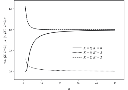
Figure 2: Matrix elements of the antisymmetrization operator for the $0^{+}$-state in ${}^{6}He$ and ${}^{6}Be$

In figure 2 overlap matrix elements diagonal in $n$ for $L=0$ and hypermomenta $K=0$ and $K=2$ are shown for the six-nucleon three-cluster system. One notices from this figure that the Pauli principle involves oscillator states of at least the 25 lowest shells, for both diagonal and off-diagonal matrix elements in $K$. The antisymmetrization effects are visible in the deviation from unity for the diagonal matrix elements, and the deviation from zero of the off-diagonal (in $K$) elements. These effects decrease monotonically with higher $n$.

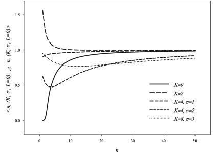
Figure 3: Matrix elements of the antisymmetrization operator for the $0^{+}$-state in ${}^{6}He$ and ${}^{6}Be$

In figure 3 we compare matrix elements for $L=0$ diagonal in $n$ and $K$ for some of the $K$-values, with $\sigma$ a multiplicity quantum number for states with identical $K$. Only those matrix elements where the Pauli principle effect is most prominent have been shown. Some states with $K=4$ and $K=8$ are affected more strongly by antisymmetrization than others. To understand this we note that the Hyperspherical angles (corresponding to the hyperangular quantum numbers $K,l_{1},l_{2},LM$) define the most probable triangular shape and orientation in space of the three-cluster system. The HH’s with $K=4,\sigma=2$ (characterized by $l_{1}=l_{2}=2$) and $K=8,\sigma=3$ (characterized by $l_{1}=l_{2}=4$) seem to describe a triangular shape where one of the nucleons is very close to the $\alpha$-particle.

For larger $K$-values the probability to find all clusters close to one another within a hypersphere of fixed radius $\rho$ decreases, and one can expect that HH’s with large values of $K$ will play a diminishing role in the calculations.

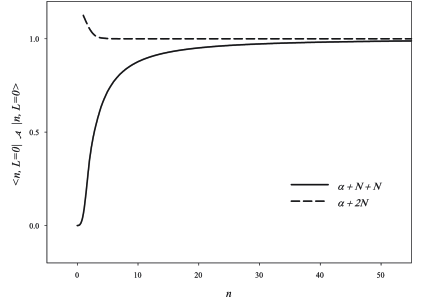
Figure 4: Matrix elements of the antisymmetrization operator for the 0⁺-state of ${}^{6}He$ and ${}^{6}Be$ in the three-cluster $\alpha+N+N$ ($K=0$) and the two-cluster configuration $\alpha+2N$

It interesting to compare overlap matrix elements for the three-cluster configuration $\alpha+N+N$ with those of the two-cluster configurations $\alpha+2N$ (such as $\alpha+d$ in ${}^{6}Li$ or $\alpha+2n$ in ${}^{6}He$). This comparison is shown in figure 4, and it indicates that the Pauli principle has a much larger “range” in the three-cluster than in the two-cluster configuration.

3.1.2 Potential matrix elements

To investigate the Pauli effect on the potential energy of the three-cluster configuration $\alpha+N+N$ we compare the potential matrix elements with hypermomentum $K=0$ with full antisymmetrization against those in the folding approximation, where antisymmetrization between clusters is neglected.

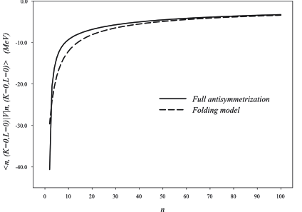
Figure 5: Diagonal potential matrix elements for the $0^{+}$-state of ${}^{6}Be$ and ${}^{6}He$ ($K=0$) with full antisymmetrization, and in the folding model

Figure 5 shows the diagonal potential matrix elements diagonal in $n$ for $K=0$ and figure 6 shows the matrix elements along a fixed row $n=50$ for $K=0$. One notes that the folding model results are very close to the fully antisymmetrized ones, especially for larger $n$.

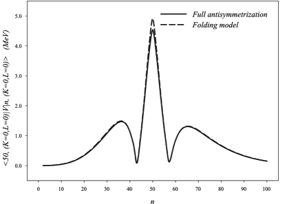
Figure 6: Off-diagonal potential matrix elements for the 0⁺-state of ${}^{6}Be$ and ${}^{6}He$ ($K=0$) with full antisymmetrization, and in the folding model

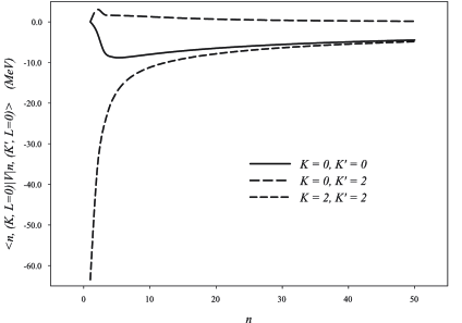
Figure 7: Diagonal potential matrix elements for the 0⁺-state of ${}^{6}Be$ and ${}^{6}He$, with full antisymmetrization

In figure 7 we also display the potential matrix elements between states of the two lowest values of hypermomentum $K=0$ and $K=2$. One notices that the $K=2$ contribution is the largest. The potential energy for $K=0$ is relatively small, and so is the coupling between $K=0$ and $K=2$ states.

The main conclusion is that, in the asymptotic region, the “exact” potential energy can be substituted with the folding approximation. It leads to a considerable reduction in computational effort. We are led to the following setup for three–cluster calculations. In the internal region, consisting of states of the lower oscillator shells and with a large probability to find the clusters close to one another, the fully antisymmetrized potential energy is used. In the asymptotic region, where the average distance between clusters is large, we use the folding model potential.

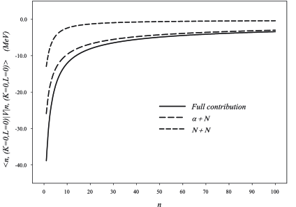
Figure 8: Folding model contributions in the diagonal potential matrix elements of the energy operator for the $0^{+}$-state of ${}^{6}Be$ and ${}^{6}He$ ($K=0$)

The folding model provides additional insight in the structure of the interaction matrix. It is well known that neither the $\alpha+n$ nor the $n+n$ interaction can create a bound state in the corresponding subsystems of ${}^{6}He$. Only a full three–cluster configuration $\alpha+n+n$ contains the necessary conditions to create a bound state. In the folding model the total potential energy is a sum of contributions from the three interacting pairs: the $\alpha$–particle and the first neutron, the $\alpha$–particle and the second neutron and the neutron-neutron pair. For $K=0$ the first two contributions are identical, and we only have to consider the $\alpha+n$ and the $n+n$ pairs. Figure 8 shows the diagonal matrix element contribution of both components, and one notices that $\alpha+n$ represents the main contribution.

3.1.3 The effective charge.

When Coulomb forces are taken into account, one needs to determine the effective charge in order to properly solve the MJM equations. The effective charge unambiguously defines the effective Coulomb interaction in each channel as well as the coupling between different channels. Using the approach suggested in section 2.1, the effective charges for the $0^{+}$- and $2^{+}$-states of ${}^{6}Be$ were calculated. Part of the corresponding matrices of $\left\|Z_{K}^{K^{\prime}}\right\|$ are displayed in tables 3 and 4 respectively. One notices that the diagonal matrix elements are much larger than the off-diagonal ones. This justifies the approximation [4] of disregarding the coupling of the channels in the asymptotic region.

Table 3: Effective charge matrix for the 0⁺-state in ${}^{6}Be$

$K;l_{1},l_{2}$	$0;0,0$	$2;0,0$	$4;0,0$	$4;2,2$
$0;0,0$	7.274	0.006	-0.129	1.414
$2;0,0$	0.006	7.146	-0.436	0.314
$4;0,0$	-0.129	-0.436	7.428	-0.877
$4;2,2$	1.414	0.314	-0.877	9.098

Table 4: Effective charge matrix for the 2⁺-state in ${}^{6}Be$

$K;l_{1},l_{2}$	$2;2,0$	$2;0,2$	$4;2,0$	$4;0,2$	$4;2,2$
$2;2,0$	7.253	0.400	-0.224	0.546	-0.751
$2;0,2$	0.400	7.244	-0.309	-0.004	-0.601
$4;2,0$	-0.224	-0.309	6.942	-0.186	0.431
$4;0,2$	0.546	-0.004	-0.186	7.694	-0.671
$4;2,2$	-0.751	-0.601	0.431	-0.671	7.345

It is interesting to compare the three-cluster effective charge with the effective charge in the two-cluster configuration. For the latter we can write

$$Z=Z_{1}Z_{2}e^{2}\sqrt{\frac{A_{1}A_{2}}{A_{1}+A_{2}}}$$

where $A_{1}$ and $Z_{1}$ ($A_{2}$ and $Z_{2}$) are the respective mass and charge of both clusters. For the configuration $\alpha+2p$ in ${}^{6}Be$, we then obtain an effective charge

$$Z=\frac{8}{\sqrt{3}}e^{2}\simeq 6.65$$

which is independent on the angular momentum of the system. One notice that the two-cluster effective charge is close to the diagonal matrix elements of $\left\|Z_{K}^{K^{\prime}}\right\|$. We can assume that, if in one of the three-cluster channels the effective charge is very close to the two-cluster one, it could indicate that the two protons move as an aggregate in the asymptotic region. For the $2^{+}$-state we observe at least one channel with this property, carrying the labels $K=4$, $l_{1}=2,$ $l_{2}=0$.

3.2 Results

3.2.1 Definition of the model space

The model space for the current calculations is primarily determined by the total number of HH’s in the internal and external region, and the number of oscillator states. Different sets of HH’s can be used in the internal and asymptotic regions. An extensive set of HH’s in the internal region will provide a well correlated description of the three-cluster system due to the coupling between states with different hypermomentum. The HH’s in the asymptotic region, which are exactly (without Coulomb) or nearly exactly (Coulomb included) decoupled, are responsible for the richness in decay possibilities.

In the current paper we restricted both internal and asymptotic HH sets maximal hypermomentum value $K_{\max}^{(i)}=K_{\max}^{(a)}=10$. By extending the respective subspaces up to these maximal values, we obtain a fair indication of convergence.

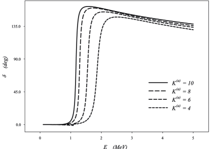
Figure 9: Eigenphase shifts for the $0^{+}$-state of ${}^{6}Be$ for different $K_{max}^{(a)}$

We fixed the matching point between internal and asymptotic region at $N=50$. It is based on the observations of the previous sections, i.e. (1) it is sufficiently large to allow the Pauli principle its full impact, and (2) it is large enough for the semi-classical approximations in the MJM to be valid.

The resonance parameters are obtained from the eigenphase shifts obtained from the eigenchannel representation (diagonalized form) of the $S$-matrix.

3.2.2 Convergence study

We first consider the influence of the number of asymptotic channels. We do this by calculating the position and width of the 0⁺-state in ${}^{6}Be$ using successively larger asymptotic subspaces. The first calculation includes all HH’s up to $K_{\max}^{(i)}=8$ and extends the asymptotic subspace from $K_{\max}^{(a)}=0$ to $K_{\max}^{(a)}=8$. The second calculation includes all HH’s up to $K_{\max}^{(i)}=10$ and extends the asymptotic subspace from $K_{\max}^{(a)}=0$ to $K_{\max}^{(a)}=10$.

Table 5: 0⁺-resonance parameters for ⁶Be, varying $K_{max}^{(a)}$ ($K_{max}^{(i)}=8$)

$K_{\max}^{(a)}$	0	2	4	6	8
$E$, MeV	1.434	1.314	1.304	1.298	1.292
$\Gamma$, MeV	0.075	0.082	0.084	0.085	0.087

Table 6: 0⁺-resonance parameters for ⁶Be, varying $K_{max}^{(a)}$ ($K_{max}^{(i)}=10$)

$K_{\max}^{(a)}$	0	2	4	6	8	10
$E$, MeV	1.324	1.204	1.192	1.184	1.176	1.172
$\Gamma$, MeV	0.068	0.069	0.071	0.071	0.073	0.072

The corresponding results are shown in tables 5 and 6. One learns from these results that a sufficient rate of convergence has been obtained. Figure 9 displays the first eigenphase shift as a function of energy for $K_{\max}^{(i)}=10$ and a choice of $K_{\max}^{(a)}$ values from which results in the tables are derived.

Table 7: 0⁺-resonance parameters for ⁶Be, varying $K_{max}^{(i)}$ ($K_{max}^{(a)}=0$)

$K_{\max}^{(i)}$	0	2	4	6	8	10
$E$, MeV	-	2.408	2.020	1.688	1.434	1.324
$\Gamma$, MeV	-	0.147	0.129	0.097	0.075	0.068

Whereas the inclusion of higher hypermomenta in the asymptotics shows a fast and monotonic convergence, it is also clear from these results that a sufficient number of HH’s has to be used for a correct description of the correlations in the internal state. To support this conclusion, we performed a calculation, again for the 0⁺-state in ${}^{6}Be$, in which only one HH with value $K^{(a)}=0$ was used. In the internal region the number of HH’s was varied from $K^{(i)}=0$ up to $K^{(i)}=10$. These results appear in table 7 and corroborate the previous conclusion. In particular they indicate that the effective potential obtained with the $K^{(i)}=0$ HH only, is unable to produce a resonance. Only after including a $K=2$ HH does the resonance appear. Further inclusion of higher HH states then lead to an acceptable convergence in a monotonically decreasing fashion for both position and width of the resonance.

Table 8: Second resonance state parameters, obtained by MJM, HHM and CSM

Nucleus	$L^{\pi}$	MJM		HH[23]		CSM[28] [29]
		$E$, MeV	$\ \Gamma$, MeV	$E$, MeV	$\Gamma$, MeV	$E$, MeV	$\Gamma$, MeV
${}^{6}He$	0${}_{2}^{+}$	2.1	4.3	5.0	6.0	3.9	9.4
${}^{6}He$	2${}_{2}^{+}$	3.7	5.0	3.3	1.2	2.5	4.7
${}^{6}Be$	0${}_{2}^{+}$	3.5	6.1
${}^{6}Be$	2${}_{2}^{+}$	5.2	5.6

Table 9: Resonance state parameters for ${}^{6}He$ and ${}^{6}Be$, obtained by MJM, HHM, CSM and CCCM

	${}^{6}He;L^{\pi}=2^{+}$		${}^{6}Be;L^{\pi}=0^{+}$		${}^{6}Be;L^{\pi}=2^{+}$
Method	$E$, MeV	$\Gamma$, MeV	$E$, MeV	$\Gamma$, MeV	$E$, MeV	$\Gamma$, MeV
MJM	1.490	0.168	1.172	0.072	3.100	0.798
HHM[23]	0.75	0.04
CSM [25]	0.74	0.06	1.52	0.16	2.81	0.87
CCCM[26]	0.73	0.07

3.2.3 Comparisons

In figure 10 we display eigenphase shifts for $L^{\pi}=0^{+}$ in ${}^{6}Be$ in the full calculations, i.e. with the maximal number of internal and asymptotic HH’s. One notices that the first $0^{+}$-resonance state of ${}^{6}Be$ appears in the first eigenchannel, and that a second (broad) resonance at a higher energy is created in the second eigenchannel (see table 8 for details on this resonance). The phase shifts in the higher eigenchannels show a smooth behavior as a function of energy without a trace of resonances in the energy range that we consider.

Table 10: Comparison of resonance state parameter in ${}^{6}He$ and ${}^{6}Be$ between MJM and experiment.

	MJM		Experiment [30]
	$E$, MeV	$\Gamma$, MeV	$E$, MeV	$\Gamma$, MeV
${}^{6}He$; $L^{\pi}=2^{+}$	1.490	0.168	0.822$\pm$0.025	0.133$\pm$0.020
${}^{6}Be$; $L^{\pi}=0^{+}$	1.172	0.072	1.371	0.092$\pm$0.006
${}^{6}Be$; $L^{\pi}=2^{+}$	3.100	0.798	3.04$\pm$0.05	1.16$\pm$0.06

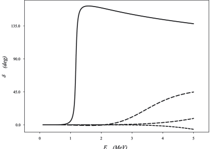
Figure 10: The eigenphases for the $0^{+}$-state in ${}^{6}Be$

Table 9 compares the results of this work to those obtained in other calculations, in particular by CSM [25], by HHM [23] and by CCCM [26]. In table 10 our results are compared with the experimental data available from [30]. The agreement with the experimental energy and width of the resonant states is reasonable. The difference between the experimental and calculated energies of the 2⁺-resonance states in both ${}^{6}He$ and ${}^{6}Be$ are probably due to the lack on LS-forces in the present calculations.

It has been pointed out in [23] and [25], that the barrier created by the three-cluster configuration is sufficiently high and wide to accommodate two resonance states, the second one usually being very broad. At first sight, this could be ascribed to an artifact of the HH Model since large values of hypermomentum $K$ create a substantial centrifugal barrier. However the CSM calculations [28, 29], which do not use HH’s, also reveal such resonances. Our calculations now also confirm the existence of a second very broad resonance. A comparison of the resonance parameters with those of the HH-method [23] and of the CSM [25] is shown in table 8. The differences are most probably due to the different descriptions of the system, as well as to the difference in $NN$-forces.

4 The ${}^{3}H(^{3}H,2n)^{4}He$ and ${}^{3}He(^{3}He,2p)^{4}He$ reactions in the MJM cluster approach

A second application that shows the strength of the MJM approach is connected to the nuclear reaction ${}^{3}He(^{3}He,2p)^{4}He$ which contributes for 89% to the $pp$-chain of nuclear synthesis, and thus is of particular interest to astrophysics. We will couple the two- and three-cluster descriptions to calculate the reaction properties, by considering a two-cluster entrance, and a three-cluster exit channel

The theoretical analysis of the ${}^{3}He(^{3}He,2p)^{4}He$ reaction is usually linked to its mirror companion, ${}^{3}H(^{3}H,2n)^{4}He$. A comparison of both leads to a better understanding of the underlying dynamics and of the Coulomb effects of reactions with three-cluster exit channels.

A first microscopic calculation for these reactions was presented in [31]. A two-cluster approach was used for both the entrance and exit channels. The nucleon-nucleon fragment cluster (denoted $NN$ for either $pp$ or $nn$) carried a simple shell-model description, featuring a pseudo-bound state with positive energy. The experimental cross-section or $S$-factor at relatively high energy (approximately 1 MeV) was reproduced by adjusting the Majorana exchange parameter of the effective $NN$-potential. The available experimental data at the (small) energy range relevant in astrophysical reactions were fairly well reproduced. In this model no resonance state appears that would sufficiently amplify the $S$-factor in the appropriate energy range, and thus would constitute an explanation for the solar neutrino problem.

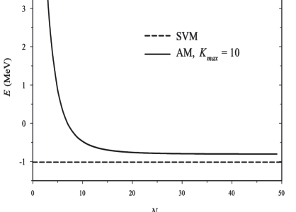
Figure 11: Ground state of ${}^{6}He$ as a function of the number of oscillator shells $N_{sh}$ in the MJM three-cluster model, compared to the results of [32]. The energy is relative to the $\alpha+n+n$ threshold.

The previous model was further improved or enhanced in [33, 34, 35] by using a more elaborate description of the $NN$-channel, or by simulating the exit channel description using both the $(^{4}He+N)+N$ and the ${}^{4}He+(N+N)$ two-cluster configurations. The relative motion of the two clusters was described by a discrete superposition of translated Gaussian functions. In each case the same $S$-factor shape as a function of energy was obtained.

In this section we study both the ${}^{3}H\left({}^{3}H,2n\right)^{4}He$ and ${}^{3}He\left({}^{3}He,2p\right)^{4}He$ reactions and use a correct treatment of the corresponding three-cluster exit channels.

The bound state energy of ${}^{6}He$ in the three-cluster description can easily be obtained by diagonalizing the nuclear Hamiltonian. We have compared it to the results obtained for the three-cluster calculation with the Stochastic Variational Method (SVM) [36] [32]. We have used the Minnesota potential without spin-orbit components, and an oscillator parameter $b=1.285$ fm which minimizes the $\alpha$-particle energy as in [32]. In figure 11 we compare our bound-state energy of ${}^{6}He$ as a function of number of oscillator shells $N_{sh}$ to the SVM value. We used all HH’s up to $K_{max}=10$. One notices convergence for $N_{sh}\geq 25$ towards $E=-0.8038$ MeV (relative to the $\alpha+n+n\$threshold). This is to be compared to $E=-1.016$ MeV for the full SVM calculation; full convergence towards the SVM result would require additional $K$ values, which is beyond the scope of the current calculation. These results encourage us to combine the two- and three-cluster MJM descriptions to obtain an advanced description of the fusion reactions ${}^{3}H(^{3}H,2n)^{4}He$ and ${}^{3}He(^{3}He,2p)^{4}He$.

4.1 Model specifics

We again rely on section 2 for the details of the microscopic model. The specific cluster configurations used to describe the six-nucleon systems ${}^{6}He$ and ${}^{6}Be$ are analogous to those of section 3.

4.1.1 A combined cluster model

The six-nucleon wave functions will be built up by using both the two- and three-cluster configurations, each one fully antisymmetrized:

$$\Psi_{L}=\mathcal{A}\left\{\Psi_{3N}~{}\Psi_{3N}~{}f_{L}\left(\mathbf{q}_{0}\right)\right\}+\mathcal{A}\left\{\Psi_{\alpha}~{}\Psi_{N}~{}\Psi_{N}~{}g_{L}\left(\mathbf{q}_{1},\mathbf{q}_{2}\right)\right\}$$ (40)

The $\Psi_{A}$ ($N$ stands for either nucleon, $\alpha$ for ${}^{4}He$, and $3N$ for ${}^{3}H$ or ${}^{3}He$) represents cluster component wave functions, $f_{L}$ and $g_{L}$ refer to the wave functions of relative motion for the two-, and three-cluster system. The $\mathbf{q}_{i}$ are Jacobi coordinates describing the configuration of relative position of the clusters.

All of the reaction dynamics, and in particular the $S$-matrix elements, is concentrated in the functions describing the relative motion, i.e. $f_{L}$ and $g_{L}$ because the internal cluster wave functions are “frozen”.

We need to make a choice for the Jacobi coordinates $\mathbf{q}$ and for a classification scheme of the wave-functions to be used in the expansion of $f_{L}$ and $g_{L}$.

For the two-cluster configuration [31] (in ${}^{3}H+^{3}H$ respectively ${}^{3}He+^{3}He$) we use the standard spherical coordinates $\mathbf{q}_{0}=\left\{q_{0},\widehat{\mathbf{q}}_{0}\right\}$ and take the quantum numbers $\mu=\{n,L,M\}$ to classify the basis states. The $n$ is the radial oscillator quantum number. As we have only central components in the $NN$ interaction, the angular momentum $L$ of relative motion will be an integral of motion for the system.

For the three-cluster configurations (in ${}^{4}He+p+p$ respectively ${}^{4}He+n+n$) we use the Hyperspherical coordinates (33). This choice is consistent with the set of quantum numbers $\nu=\left\{N,K,(l_{1}l_{2})LM\right\}=\left\{n_{\rho},K,(l_{1}l_{2})LM\right\}$, in which $N=2n_{\rho}+K$ represents the total number of oscillator quanta, and $n_{\rho}$ reflects the number of hyperradial excitations. The partial angular momenta $l_{1}$ and $l_{2}$ are associated with the choice of Jacobi vectors $\mathbf{q}_{1}$ and $\mathbf{q}_{2}$. A coupled $K$-channel calculation with each channel characterized by the set of quantum numbers $\nu_{0}=\left\{K,(l_{1}l_{2})LM\right\}$, has to be performed. This type of basis is particularly suitable for the so-called Borromian nuclei, and nuclei with pronounced three-cluster features, when the three-cluster threshold represents the lowest energy decay channel.

4.1.2 The boundary conditions

The MJM boundary conditions are expressed in terms of the expansion coefficients of the wave functions of relative motion. They are directly connected to the boundary conditions in coordinate representation. For the two-cluster configurations the asymptotic form of the expansion coefficients in $f_{L}=\sum c_{n,L}\phi_{n,L}$ can be approximated by

$$c_{n,L}\simeq\sqrt{r_{n}}f_{L}\left(r_{n}\right)$$ (41)

where the $\{\phi_{n,L}\}$ are the oscillator basis functions, and $r_{n}=b\sqrt{4n+2L+3}$ is the classical turning point of the three-dimensional oscillator with energy $E_{n}=\hbar\omega\left(2n+L+3/2\right)$. In three-cluster configurations the expansion is defined by $g_{L}=\sum d_{n_{\rho},L}\phi_{n_{\rho},L}$, where the $\{\phi_{n_{\rho},L}\}$ now stand for the oscillator basis for three-cluster relative motion. The expansion coefficients behave asymptotically as

$$d_{n_{\rho},L}\simeq\sqrt{2}\rho_{n}^{2}g_{L}\left(\rho_{n}\right)$$ (42)

with $\rho_{n}=b\sqrt{4n_{\rho}+2K+6}$. For clarity we have indicated in the preceding discussion only relevant indices to this section.

We consider both incoming and outgoing waves for the two-cluster configurations

$$f_{L}\left(\mathbf{q}_{0}\right)\simeq\left[\psi_{L}^{\left(-\right)}\left(k_{0}q_{0}\right)-S_{\{\mu\},\{\mu\}}~{}\psi_{L}^{\left(+\right)}\left(k_{0}q_{0}\right)\right]Y_{LM}\left(\widehat{\mathbf{q}}_{0}\right)$$ (43)

where $S_{\{\mu\},\{\mu\}}$ is a notation to characterize the elastic two-cluster scattering matrix element for the ${}^{3}H+^{3}H$, resp. ${}^{3}He+^{3}He$ channels, and $Y_{LM}\left(\widehat{\mathbf{q}}_{0}\right)$ is the spherical harmonic.

Because we are only interested in reactions with a three-cluster exit-channel, the asymptotic wave function can be written as

$$g_{L}\left(\mathbf{q}_{1},\mathbf{q}_{2}\right)=g_{L}\left(\rho\mathbf{,}\Omega\right)\simeq\sum_{\nu_{0}}\left[-S_{\{\mu\},\{\nu_{0}\}}~{}\psi_{K}^{\left(+\right)}\left(k\rho\right)\right]H_{K}^{\nu_{0}}\left(\Omega\right)$$ (44)

where $S_{\{\mu\},\{\nu_{0}\}}$ is the scattering matrix element describing the inelastic coupling between the two- and three-cluster channels, and $H_{K}^{\nu_{0}}\left(\Omega\right)$ is the HH.

The total cross-section is given by the expression

$$\sigma\left(E\right)=\frac{\pi}{k_{0}^{2}}\sum_{L,S}\frac{\left(2L+1\right)\left(2S+1\right)}{4}\sum_{\nu_{0}}\left|S_{\{\mu\},\{\nu_{0}\}}\right|^{2}$$ (45)

with $S$ the total spin of the six-nucleon system.

As discussed in section 2.1, the asymptotic solutions for incoming and outgoing waves can be written as

$$\psi_{\mathcal{L}}^{\left(\pm\right)}\left(k\rho\right)=\frac{1}{\sqrt{k}}W_{\pm i\eta,\lambda}\left(\pm 2ik\rho\right)/\rho^{\frac{\sigma-1}{2}}$$ (46)

where $W$ are the Whittaker functions, and $\eta$ the Sommerfeld parameter (for the parameters $\mathcal{L}$, $\lambda$, $\sigma$ and $\eta$ for two- and three-cluster channels: see table 2).

By using the correspondences (41) and (42) we can now define the boundary conditions for the expansion coefficients

$$c_{n,L} \simeq\sqrt{r_{n}}\left[\psi_{L}^{\left(-\right)}\left(k_{0}r_{n}\right)-S_{\{\mu\},\{\mu\}}~{}\psi_{L}^{\left(+\right)}\left(k_{0}r_{n}\right)\right]$$

$$d_{n_{\rho},\nu_{0}} \simeq\rho_{n}^{2}\left[-S_{\{\mu\},\{\nu_{0}\}}~{}\psi_{K}^{\left(+\right)}\left(k\rho_{n}\right)\right]$$ (47)

or equivalently

$$c_{n,L} \simeq c_{n,L}^{\left(-\right)}-S_{\{\mu\},\{\mu\}}~{}c_{n,L}^{\left(+\right)}$$

$$d_{n_{\rho},\nu_{0}} \simeq-S_{\{\mu\},\{\nu_{0}\}}~{}c_{n_{\rho},\nu_{0}}^{\left(+\right)}$$ (48)

using the notations

$$c_{n,L}^{\left(\pm\right)} \simeq\sqrt{r_{n}}\psi_{L}^{\left(\pm\right)}\left(k_{0}r_{n}\right)$$

$$d_{n_{\rho},\nu_{0}}^{\left(\pm\right)} \simeq\rho_{n}^{2}~{}\psi_{K}^{\left(\pm\right)}\left(k\rho_{n}\right)$$ (49)

The matching of internal and asymptotic regions is equivalent to the one in the traditional Resonating Group Method (RGM). The correspondence between the matching point in coordinate space for RGM and in function space for MJM is easily made (see [4]) through the value of the classical oscillator turning point $r_{n}=b\sqrt{4n+2L+3}$ for 2-cluster systems and $\rho_{n}=b\sqrt{4n_{\rho}+2K+6}$ for 3-cluster systems. An appropriate value for the matching point can be obtained by choosing sufficiently large values for the total number of oscillator quanta $N=2n+L=2n_{\rho}+K$ in the internal region.

4.1.3 Shape analysis

The HH’s can reveal information on the spatial distribution of clusters and of the reaction dynamics.

These harmonics define a probability distribution in 5-dimensional coordinate (momentum) space for fixed values of hyperradius:

$$dW_{\nu_{0}}^{5}\left(~{}\Omega\right)=\left|Y_{\nu_{0}}\left(~{}\Omega\right)\right|^{2}d\Omega,\quad dW_{\nu_{0}}^{5}\left(~{}\Omega_{k}\right)=\left|Y_{\nu_{0}}\left(~{}\Omega_{k}\right)\right|^{2}d\Omega_{k}$$ (50)

By analyzing the probability distribution, one can retrieve the most probable shape of three-cluster shape or “triangle” of clusters. A full analysis of a function of 5 variables is non-trivial and one usually restricts oneself to some specific variable(s). We integrate the probability distribution $dW_{\nu_{0}}^{5}\left(~{}\Omega\right)$ over the unit vectors $\widehat{\mathbf{q}}_{1},\widehat{\mathbf{q}}_{2}$ (resp. $\widehat{\mathbf{k}}_{1},\widehat{\mathbf{k}}_{2}$)

$$dW_{\nu_{0}}\left(\theta\right) =\int\left|Y_{\nu_{0}}\left(~{}\Omega\right)\right|^{2}\cos^{2}\theta\sin^{2}\theta d\theta~{}d\widehat{\mathbf{q}}_{1}d\widehat{\mathbf{q}}_{2}$$

$$dW_{\nu_{0}}\left(\theta_{k}\right) =\int\left|Y_{\nu_{0}}\left(~{}\Omega_{k}\right)\right|^{2}\cos^{2}\theta_{k}\sin^{2}\theta_{k}d\theta_{k}~{}d\widehat{\mathbf{k}}_{1}d\widehat{\mathbf{k}}_{2}$$ (51)

and introduce the (new) variable(s)

$$\mathcal{E}=\frac{q_{1}^{2}}{\rho^{2}}=\cos^{2}\theta,\quad\mathcal{E}=\frac{k_{1}^{2}}{k^{2}}=\cos^{2}\theta_{k}$$

In coordinate space these can be interpreted as the squared distance between the pair of clusters associated with coordinate $\mathbf{q}_{1}$, or, in momentum space, the relative energy of that pair of clusters. We obtain

$$W_{\nu_{0}}\left(\mathcal{E}\right) =\frac{dW_{\nu_{0}}\left(\theta\right)}{d\theta}=\left|N_{K}^{\left(l_{1},l_{2}\right)}\cos^{l_{1}}\theta\sin^{l_{2}}\theta P_{n}^{\left(l_{2}+1/2,l_{1}+1/2\right)}\left(\cos 2\theta\right)\right|^{2}\cos^{2}\theta\sin^{2}\theta$$

$$=\left|N_{K}^{\left(l_{1},l_{2}\right)}\left(\mathcal{E}\right)^{l_{1}/2}\left(1-\mathcal{E}\right)^{l_{2}/2}P_{n}^{\left(l_{2}+1/2,l_{1}+1/2\right)}\left(2\mathcal{E}-1\right)\right|^{2}\sqrt{\mathcal{E}\left(1-\mathcal{E}\right)}$$ (52)

This function represents the probability distribution for relative distance between the two clusters, resp. for the energy of relative motion of the two clusters. The kinematical factor $\cos^{2}\theta\sin^{2}\theta$ was included to make $W_{\nu_{0}}\left(\mathcal{E}\right)$ proportional to the differential cross section in momentum space, provided the exit channel is described by the single HH $Y_{\nu_{0}}\left(\Omega\right)$.

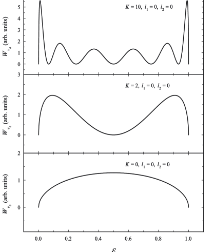
Figure 12: Function $W_{\nu_{0}}\left(\mathcal{E}\right)$ for $K=0,\ 2$ and $10$ and $l_{1}=l_{2}=0$.

In figure 12 we display $W_{\nu_{0}}\left(\mathcal{E}\right)$ for some HH’s involved in our calculations. These figures show that different HH’s account for different shapes of the three-cluster systems. For instance, the HH with $K=10$ and $l_{1}=l_{2}=0$ prefers the two clusters to move with very small or very large relative energy, or, in coordinate space, prefers them to be close to each other, or far apart.

4.2 Results

Again we use the VP as the $NN$ interaction. The Majorana exchange parameter $m$ was set to be $0.54$ which is comparable to the one used in [34]. The oscillator radius was set to $b=1.37$ fm (as in [5, 7]) to optimize the ground state energy of the alpha-particle.

The VP does not contain spin-orbital or tensor components so that total angular momentum $L$ and total spin $S$ are good quantum numbers. Moreover, due to the specific features of the potential, the binary channel is uncoupled from the three-cluster channel when the total spin $S$ equals 1; this means that odd parity states $L^{\pi}=1^{-},2^{-},\ldots$ will not contribute to the reactions.

Table 11: Number of Hyperspherical Harmonics for $L=0$.

$N_{ch}$	1	2	3	4	5	6	7	8	9	10	11	12
$K$	0	2	4	4	6	6	8	8	8	10	10	10
$l_{1}=l_{2}$	0	0	0	2	0	2	0	2	4	0	2	4

To describe the continuum of the three-cluster configurations we considered all HH’s with $K\leq K_{max}=10$. In Table 11 we enumerate all contributing $K$-channels for $L=0$. For each two- and three-cluster channel we used the same number $n=n_{\rho}=N_{int}$ of basis functions to describe the internal part of the wave function $\Psi_{L}$. $N_{int}$ then also defines the matching point between the internal and asymptotic part of the wave function. We used $N_{int}$ as a variational parameter and varied it between 20 and 75, which corresponds to a variation in coordinate space of the RGM matching radius approximately between 14 and 25 fm. This variation showed only small changes in the $S$-matrix elements, of the order of one percent or less, and do not influence any of the physical conclusions. We have then used $N_{int}=25$ for the final calculations as a compromise between convergence and computational effort. We also checked the impact of $N_{int}$ on the unitarity conditions of the $S$-matrix, for instance the relation

$$\left|S_{\{\mu\},\{\mu\}}\right|^{2}+\sum_{\nu_{0}}\left|S_{\{\mu\},\{\nu_{0}\}}\right|^{2}~{}=1$$

We have established that from $N_{int}=15$ on this unitarity requirement is satisfied with a precision of one percent or better. In our calculations, with $N_{int}=25$, unitarity was never a problem. It should be noted that our results concerning the convergence for the three-cluster system with a restricted basis of oscillator functions agree with those of Papp et al [37], where a different type of square-integrable functions was used for three-cluster Coulombic systems.

In figure 13 we show the total $S$-factor for the reaction ${}^{3}H\left({}^{3}H,2n\right)^{4}He$ in the energy range $0\leq E\leq 200$ keV. One notices that the theoretical curve is very close to the experimental data.

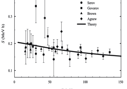
Figure 13: $S$-factor of the reaction ${}^{3}H\left({}^{3}H,2n\right)^{4}He$. Experimental data are taken from [38](Serov), [39] (Govorov),[40] (Brown) and [41] (Agnew)

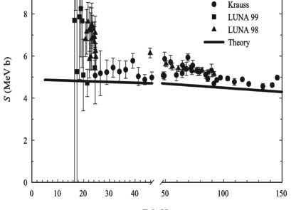
Figure 14: $S$-factor of the reaction ${}^{3}He\left({}^{3}He,2p\right)^{4}He$. Experimental data are from [42] (Krauss), [43] (LUNA 99) and [44] (LUNA 98).

The total $S$-factor for the reaction ${}^{3}He\left({}^{3}He,2p\right)^{4}He$ is displayed in figure 14. It is also close to the available experimental data. The $S$-factor for both reactions is seen to be a monotonic function of energy, and does not manifest any irregularities to be ascribed to a hidden resonance. Thus no indications are found towards explaining the solar neutrino problem.

The astrophysical $S$-factor at small energy is usually written as

$$S\left(E\right)=S_{0}+S_{0}^{\prime}E+S_{0}^{\prime\prime}E^{2}$$ (53)

We have fitted the calculated $S$-factor to this formula in the energy range $0\leq E\leq 200$ keV. For the reaction ${}^{3}H\left({}^{3}H,2n\right)^{4}He$ we obtain the approximate expression:

$$S\left(E\right)=206.51-0.53~{}E+0.001~{}E^{2}\quad\text{keV b}$$ (54)

and for ${}^{3}He\left({}^{3}He,2p\right)^{4}He$ we find:

$$S\left(E\right)=4.89-3.99~{}E+2.3~{}~{}10^{-4}~{}E^{2}\quad\text{MeV b}$$ (55)

One notices significant differences in the $S$-factor for the ${}^{6}He$ and ${}^{6}Be$ systems. The $NN$-interaction induces the same coupling between the clusters of entrance and exit channels for both ${}^{6}He$ and ${}^{6}Be$. It is the Coulomb interaction that distinguishes both systems, and accounts for the pronounced differences in the cross-sections and $S$-factors.

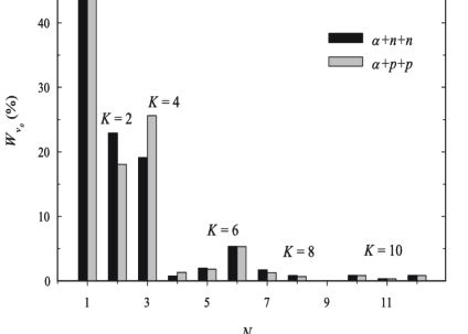
Figure 15: Three-cluster channel contributions to the total $S$-factor for the reactions ${}^{3}H\left({}^{3}H,2n\right)^{4}He$ and ${}^{3}He\left({}^{3}He,2p\right)^{4}He$ in a full calculation with $K_{max}=10$.

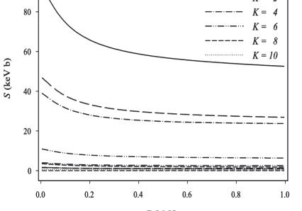
Figure 16: Three-cluster channel contributions to the total $S$-factor of the reactions ${}^{3}H(^{3}H,2n)^{4}He$ in a full calculation with $K_{max}=10$, in the energy range $0\leq E\leq 1000$ keV.

We compare the calculated $S$-factor to fits of experimental results for the reaction ${}^{3}He\left({}^{3}He,2p\right)^{4}He$:

$$S\left(E\right) =5.2-2.8~{}E+1.2~{}E^{2}\quad\text{MeV b \cite[cite]{[\@@bibref{}{kn:dwarakanath71}{}{}]}}$$

$$S\left(E\right) =\left(5.40\pm 0.05\right)-\left(4.1\pm 0.5\right)E+\left(2.3\pm 0.5\right)E^{2}\quad\text{MeV b\cite[cite]{[\@@bibref{}{Arpesella:1997zf}{}{}]}}$$

$$S\left(E\right) =\left(5.32\pm 0.08\right)-\left(3.7\pm 0.6\right)E+\left(1.95\pm 0.5\right)E^{2}\quad\text{MeV b \cite[cite]{[\@@bibref{}{Bonetti:1999yt}{}{}]}}$$ (56)

The constant and linear terms of the fit display a good agreement. The difference in energy ranges between the calculated ($0\leq E\leq 200$ keV) and experimental ($0\leq E\leq 1000$ keV) fits make it difficult to attribute any significant interpretation to the discrepancy in the quadratic term.

The HH’s method now allows to study some details of the dynamics of the reactions considered.

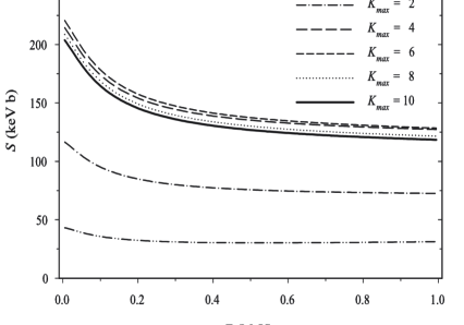
Figure 17: Convergence of the $S$-factor of the reaction ${}^{3}H(^{3}H,2n)^{4}He$ for $K_{max}$ ranging from $0$ to $10$.

In Figs. 15 and 16 we show the different three-cluster $K$-channel contributions ($W_{\nu_{0}}$) to the total $S$-factor of the reactions. In figure 15 these contributions (in % with respect to the total $S$-factor) are displayed for some fixed energy (1 keV), while figure 16 shows the dependency of $W_{\nu_{0}}$ (in absolute value) on the energy of the entrance channel. One notices that three HH’s dominate the full result, namely the $\left\{K=0;l_{1}=l_{2}=0\right\}$, $\left\{K=2;l_{1}=l_{2}=0\right\}$ and $\left\{K=4;l_{1}=l_{2}=2\right\}$, and this is true in both reactions. The contribution of these states to the $S$-factor is more then 95 % . There also is a small difference between the reactions ${}^{3}H\left({}^{3}H,2n\right)^{4}He$ and ${}^{3}He(^{3}He,2p)^{4}He$, which is completely due to the Coulomb interaction.

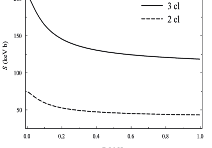
Figure 18: Comparison of the $S$-factor of the reaction ${}^{3}H(^{3}H,2n)^{4}He$ in a calculation with a three-cluster exit-channel and a pure two-cluster model.

The Figs. 15 and 16 yield an impression of the convergence of the results. We notice that the contribution of the HH’s with $K>6$ is small compared to the dominant ones. This is corroborated in figure 17 where we show the rate of convergence of the $S$-factor in calculations with $K_{max}$ ranging from $0$ up to $10$. Our full $K_{max}=10$ basis is seen to be sufficiently extensive to account for the proper rearrangement of two-cluster configurations into a three-cluster one, as the differences between results becomes increasingly smaller.

To emphasize the importance for a correct three-cluster exit-channel description, we compare the present calculations to those in [31], where only two-cluster configurations ${}^{4}He+2n$ resp. ${}^{4}He+2p$ were used to model the exit channels. In both calculations we used the same interaction and value for the oscillator radius. In figure 18 we compare both results for ${}^{3}H(^{3}H,2n)^{4}He$. An analogous picture is obtained for the reaction ${}^{3}He(^{3}He,2p)^{4}He$.

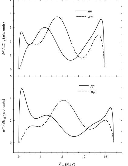
Figure 19: Partial differential cross sections of the reactions ${}^{3}H(^{3}H,2n)^{4}He$ and ${}^{3}He(^{3}He,2p)^{4}He$.

4.2.1 Cross sections

Having calculated the $S$-matrix elements, we can now easily obtain the total and differential cross sections. In this section we will calculate and analyze one-fold differential cross sections, which define the probability for a selected pair of clusters to be detected with a fixed energy $E_{12}$. To do so we shall consider a specific choice of Jacobi coordinates in which the first Jacobi vector $\mathbf{q}_{1}$ is connected to the distance between these clusters, and the modulus of vector $\mathbf{k}_{1}$ is the square root of relative energy $E_{12}$. With this definition of variables, the cross section is

$$d\sigma\left(E_{12}\right)\sim\frac{1}{E}\int d\widehat{\mathbf{k}}_{1}d\widehat{\mathbf{k}}_{2}\left|\sum_{\nu_{0}}S_{\{\mu\}\{\nu_{0}\}}Y_{\nu_{0}}\left(\Omega_{k}\right)\right|^{2}\sin^{2}\theta_{k}\cos^{2}\theta_{k}d\theta_{k}$$ (57)

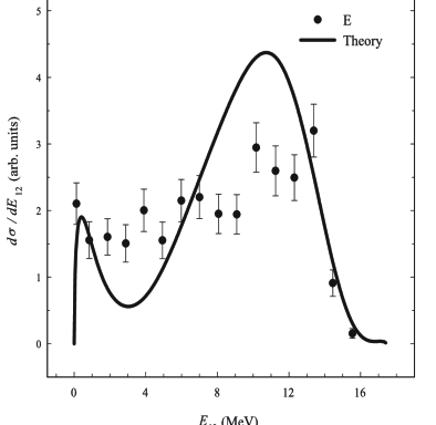
Figure 20: Calculated and experimental differential cross section for the reaction ${}^{3}He(^{3}He,2p)^{4}He$. Experimental data is taken from [45].

After integration over the unit vectors and substitution of $\sin\theta_{k}$, $\cos\theta_{k}$, $d\theta_{k}$ with

$$\cos\theta_{k} =\sqrt{\frac{E_{12}}{E}};\quad\sin\theta_{k}=\sqrt{\frac{E-E_{12}}{E}}$$

$$d\theta_{k} =\frac{1}{2}\frac{1}{\sqrt{\left(E-E_{12}\right)E_{12}}}dE_{12}$$ (58)

one can easily obtains $d\sigma\left(E_{12}\right)/dE_{12}.$

In figure 19 we display the partial differential cross sections of the reactions ${}^{3}H\left({}^{3}H,2n\right)^{4}He$ and ${}^{3}He\left({}^{3}He,2p\right)^{4}He$ for the energy $E=10$ keV in the entrance channel. The solid lines correspond to the case of two neutrons (protons) with relative energy $E_{12}$, while the dashed lines represent the cross sections of the $\alpha$-particle and one of the neutrons (protons) with relative energy $E_{12}$.

We wish to emphasize the cross section in which two neutrons or two protons are simultaneously detected. One notices a pronounced peak in the cross section around $E_{12}\simeq 0.5$ MeV. This peak is even more pronounced for the reaction ${}^{3}He\left({}^{3}He,2p\right)^{4}He$. It means that at such energy two neutrons or two protons could be detected simultaneously with large probability. We believe that this peak can explain the relative success of a two-cluster description for the exit channels at that energy. The pseudo-bound states of $nn$- or $pp$-subsystems used in this type of calculation then allows for a reasonable approximation of the astrophysical $S$-factor.

Special attention should be paid to the energy range 1-3 MeV in the ${}^{4}He+n$ and ${}^{4}He+p$ subsystems. This region includes $3/2^{-}$ and $1/2^{-}$ resonance states of these subsystems with the Volkov potential. In figure 19 (dashed lines) we see that it yields a small contribution to the cross sections of the reactions ${}^{3}H\left({}^{3}H,2n\right)^{4}He$ and ${}^{3}He\left({}^{3}He,2p\right)^{4}He$. This contradicts the conclusions of [34] and [35] where the $1/2^{-}$ state of the ${}^{4}He+N$ subsystem played a dominant role. We suspect this dominance to be due to the interplay of two factors: the weak coupling between incoming and outgoing channels, and the spin-orbit interaction.

In figure 20 we compare our results for the total proton yield (reaction ${}^{3}He\left({}^{3}He,2p\right)^{4}He$) to the experimental data from [45]. The latter were obtained for incident energy $E\left({}^{3}He\right)=0.19$ MeV. One notices a qualitative agreement between the calculated and experimental data.

The cross sections, displayed in Figs. 19 and 20, were obtained with the maximal number of HH’s ($K\leq 10$). These figures should now be compared to the figure 12, which displays partial differential cross sections for a single $K$-channel. The cross sections, displayed in Figs. 19 and 20, differ considerably from those in Figs. 12 and comparable ones, even for those HH’s which dominate the wave functions of the exit channel. An analysis of the cross section shows that the interference between the most dominant HH’s strongly influences the cross-section behavior. To support this statement we display the proton cross sections obtained with hypermomenta $K=0$, $K=2$, $K=4$ to those obtained with the full set of most important components $K_{max}\leq 4$ in figure 21. One observes a huge bump around 10 MeV which is entirely due the interference of the different HH components. We also included the full calculation ($K_{max}\leq 10$) to indicate the rate of convergence for this cross-section.

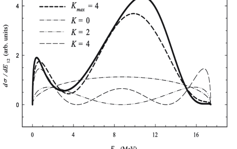
Figure 21: Partial cross sections for the reaction ${}^{3}He(^{3}He,2p)^{4}He$ obtained for individual $K=0,2$ and $4$ components, compared to the coupled calculation with $K_{max}=4$ and the full calculations with $K_{max}=10$.

5 Conclusion

In this paper we have presented a three-cluster description of light nuclei on the basis of the Modified J-Matrix method (MJM). Key steps in the MJM calculation of phase shifts and cross sections have been analyzed, in particular the issue of convergence. Results have been reported for ${}^{6}He$ and ${}^{6}Be$. They compare favorably to available experimental data. We have also reported results for coupled two- and three-cluster MJM calculations for the ${}^{3}He\left({}^{3}He,2p\right)^{4}He$ and ${}^{3}H\left({}^{3}H,2n\right)^{4}He$ reactions with three-way disintegration. Again comparison indicates good agreement with other calculations and with experimental data.

References

- [1] W. Vanroose, J. Broeckhove, and F. Arickx. Modified J-Matrix Method for Scattering. Physical Review Letters, 88:10404–+, January 2002.
- [2] V. S. Vasilevsky and F. Arickx. Algebraic model for quantum scattering: Reformulation, analysis, and numerical strategies. Phys. Rev., A55:265–286, 1997.
- [3] V. Vasilevsky, G. Filippov, F. Arickx, J. Broeckhove, and P. Van Leuven. Coupling of collective states in the continuum: an application to 4He. J. Phys. G: Nucl. Phys., G18:1227–1242, 1992.
- [4] V. S. Vasilevsky, A. V. Nesterov, F. Arickx, and J. Broeckhove. Algebraic model for scattering in three-s-cluster systems. I. Theoretical background. Phys. Rev., C63:034606, 2001.
- [5] V. S. Vasilevsky, A. V. Nesterov, F. Arickx, and J. Broeckhove. Algebraic model for scattering in three--cluster systems. II. Resonances in three-cluster continuum of and . Phys. Rev., C63:034607, 2001.
- [6] V. S. Vasilevsky, A. V. Nesterov, F. Arickx, and P. Van Leuven. Dynamics of channel in 6He and 6Li. Preprint ITP-96-3E, page 19, 1996.
- [7] V. S. Vasilevsky, A. V. Nesterov, F. Arickx, and P. Van Leuven. Three-cluster model of six-nucleon system. , 60:413–419, 1997.
- [8] Yu. A. Simonov. Sov. J. Nucl. Phys., 7:722, 1968.
- [9] M. Fabre de la Ripelle. Green function and scattering amplitudes in many-dimensional space. Few-Body Systems, 14:1–24, 1993.
- [10] M. V. Zhukov et al. Phys. Rep., 231:151, 1993.
- [11] F. Zernike and H. C. Brinkman. Proc. Kon. Acad. Wetensch., 33:3, 1935.
- [12] I. F. Gutich, A. V. Nesterov, and I. P. Okhrimenko. Yad. Fiz., 50:19, 1989.
- [13] T.Ya.Mikhelashvili, Yu. F. Smirnov, and A. M. Shirokov. The continuous spectrum effect on monopole excitations of the 12C nucleus considered as a system of a particles. Sov. J. Nucl. Phys., 48:969, 1988.
- [14] E. J. Heller and H. A. Yamani. New approach to quantum scattering: Theory. Phys. Rev., A9:1201–1208, 1974.
- [15] H. A. Yamani and L. Fishman. -matrix method: Extensions to arbitrary angular momentum and to Coulomb scattering. J. Math. Phys., 16:410–420, 1975.
- [16] Y. I. Nechaev and Y. F. Smirnov. Solution of the scattering problem in the oscillator representation. Sov. J. Nucl. Phys., 35:808–811, 1982.
- [17] A. M. Perelomov. Commun. Math. Phys., 26:222, 1972.
- [18] A. M. Perelomov. Generalized Coherent States and their Applications. Springer, Berlin, 1987.
- [19] F. Arickx, J. Broeckhove, P. Van Leuven, V. Vasilevsky, and G. Filippov. The algebraic method for the quantum theory of scattering. Amer. J. Phys., 62:362–370, 1994.
- [20] D. V. Fedorov, A. S. Jensen, and K. Riisager. Three-body halos: Gross properties. Phys. Rev., C49:201–212, 1994.
- [21] F. Calogero. Variable Phase Approach to Potential Scattering. Academic Press, New-York and London, 1967.
- [22] V. V. Babikov. Phase Function Method in Quantum Mechanics. Nauka, Moscow, 1976.
- [23] B. V. Danilin et al. Dynamical multicluster model for electroweak and charge-exchange reactions. Phys. Rev., 1991:2835–2843, C43.
- [24] B.V.Danilin, T.Rogde, S.N.Ershov, H.Heiberg-Andersen, J.S.Vaagen, I.J.Thompson, and M.V.Zhukov. New modes of halo excitation in 6He nucleus. Phys. Rev., C55:R577–R581, 1997.
- [25] A. Csoto. Three-body resonances in 6He, 6Li, and 6Be, and the soft dipole mode problem of neutron halo nuclei. Phys. Rev., C49:3035–3041, 1994.
- [26] N. Tanaka, Y. Suzuki, and K. Varga. Exploration of resonances by analytical continuation in the coupling constant. Phys. Rev., C56:562–565, 1997.
- [27] A. B. Volkov. Equilibrum deformation calculation of the ground state energies of 1p shell nuclei. Nucl. Phys., 74:33–58, 1965.
- [28] S. Aoyama et al. Progr. Theor. Phys., 93:99, 1995.
- [29] S. Aoyama et al. Progr. Theor. Phys., 94:343, 1995.
- [30] F. Ajzenberg-Selove. Nucl. Phys., A490:1, 1988.
- [31] V. S. Vasilevsky and I. Yu. Rybkin. Sov. J. Nucl. Phys., 50:411, 1989.
- [32] Y. Suzuki K. Varga and R. G. Lovas. Microscopic multicluster description of neutron-halo nuclei with a stochastic variational method. Nucl. Phys, A571:447–466, 1994.
- [33] S. Typel, G. Bluge, K. Langanke, and W. A. Fowler. Microscopic study of the low-energy 3He(3He,2p)4He and 3H(3H,2n)4He fusion cross sections. Z. Phys., A339:249, 1991.
- [34] P. Descouvemont. Microscopic analysis of the and reactions in a three-cluster model. Phys. Rev., C50:2635–2638, 1994.
- [35] A. Csoto and K. Langanke. Large-space cluster model calculations for the 3He(3He,2)4He and 3H(3H,2)4He reactions. Nucl. Phys., A646:387, 1999.
- [36] K. Varga and Y. Suzuki. Precise solution of few body problems with stochastic variational method on correlated gaussian basis. Phys. Rev., C52:2885–2905, 1995.
- [37] Z. Papp, I. N. Filikhin, and S. L. Yakovlev. Integral equations for three-body Coulombic resonances. Few Body Syst. Suppl., 99:1, 1999.
- [38] V. I. Serov, S. N. Abramovich, and L. A. Morkin. Sov. J. At. Energy, 42:66, 1977.
- [39] A.M.Govorov, L. Ka-Yeng, G. M. Osetinskii, V. I. Salatskii, and I. V. Sizov. Sov. Phys. JETP, 15:266, 1962.
- [40] R. E. Brown and N. Jarmie. Radiat. Eff., 84:45, 1986.
- [41] H.M.Agnew, W.T.Leland, H.V.Argo, R.W.Crews, A.H.Hemmendinger, W.E.Scott, and R.F.Taschek. Measurement of the cross section for the reaction + 11.4 MeV. Phys. Rev., 84:862–863, 1951.
- [42] A. Krauss, H. W. Becker, H. P. Trautvetter, and C. Rolfs. Astrophysical factor of at solar energies. Nucl. Phys., A467:273–290, 1987.
- [43] The LUNA Collaboration. First measurement of the cross section down to the lower edge of the solar gamow peak. Preprint, nucl-ex/9902004, 1999.
- [44] M. Junker The LUNAC̃ollaboration, A. D’Alessandro, S. Zavatarelli, C. Arpesella, E. Bellotti, C. Broggini, P. Corvisiero, G. Fiorentini, A. Fubini, and G. Gervino. The cross section of measured at solar energies. Phys. Rev., C57:2700–2710, 1998.
- [45] M. R. Dwarakanath and H. Winkler. total cross-section measurements below the Coulomb barrier. Phys. Rev., C4:1532–1540, 1971.
- [46] C. Arpesella et al. The cross section of measured at solar energies. Phys. Rev., C57:2700–2710, 1998.
- [47] R. Bonetti et al. First measurement of the cross section down to the lower edge of the solar gamow peak. Phys. Rev. Lett., 82:5205–5208, 1999.