Theoretical analysis of resonance states in ${}^{4}H$, ${}^{4}He$ and ${}^{4}Li$ above three-cluster threshold

Abstract

The resonance states of ${}^{4}H$, ${}^{4}He$ and ${}^{4}Li$, embedded in the three-cluster $d+N+N$ continuum, are investigated within a three-cluster model. The model treats the Pauli principle exactly and incorporates the Faddeev components for proper description of the boundary conditions for the two- and three-body continua. The hyperspherical harmonics are used to distinguish and numerate channels of the three-cluster continuum. It is shown that the effective barrier, created by three-cluster configuration $d+N+N$, is strong enough to accommodate two resonance states.

UDC 539.142

1 Introduction

In this paper we study the nature of resonance states in ${}^{4}H$, ${}^{4}He$ and ${}^{4}Li$. All these nuclei have a rich structure of resonance states [1]. There are 4 well-determined resonances in ${}^{4}H$ and ${}^{4}Li$, and up to 15 resonance states were detected in ${}^{4}He$. Most of these resonances have a width that is much larger than the resonance energy when measured from the lowest threshold. Although these resonances have been experimentally confirmed, they can hardly be observed in current theoretical model descriptions of these systems through standard elastic and inelastic scattering quantities such as $S$-matrix elements, differential or total cross sections, and so on.

For many years, the four-nucleon system was studied by different microscopic and semi-microscopic methods. Different forms of the Schrödinger equation (differential ([2, 3]), integral ([4, 5, 6]), integro-differential [7, 8, 9, 10], matrix or algebraic([11, 12, 13]), …) have been used to study these nuclei. Special attention was paid to ${}^{4}He$, the only nuclear 4-particle system featuring a bound state. The theoretical study of the “ground state” of ${}^{4}H$ and ${}^{4}Li$, and of the excited states of all three nuclei were investigated mainly through resonance state analysis. Of all resonances, the first excited $0^{+}$ state has received most attention. In none of the descriptions the role of the three-cluster channels was properly considered, and so resonance states induced by this channel could not be theoretically discovered and analyzed.

Our objective is to determine the type and nature of resonance states in ${}^{4}H$, ${}^{4}He$ and ${}^{4}Li$ that are reproduced within a three-cluster microscopic model. For all three nuclei we will consider one single three-cluster configuration $d+N+N$. This is certainly the most dominant three-cluster channel, as it has the lowest energy threshold. Moreover one can easily construct all binary channels for these nuclei within such description. In ${}^{4}He$ for example this configuration allows to study resonances created by the two-cluster channels $p+^{3}H$, $n+^{3}He$ and $d+d$, as well as by the three-cluster channel $d+p+n$. The latter should be very important, because 7 resonance states were detected above the $d+p+n$ threshold. It is interesting to note in the same context that all four resonance states of ${}^{4}H$ lie below the three-cluster $d+n+n$ threshold, whereas in ${}^{4}Li$ two resonances are found above the $d+p+p$ threshold.

We propose a modification of the method formulated in [14, 15, 16], and used in [17, 18] to study resonances embedded in the three-cluster continuum, and reactions with three cluster exit channels. The method was shown to provide a suitable instrument for investigating Borromian nuclei (for instance ${}^{6}He$) and nuclei with prominent three-cluster features (like ${}^{6}Be$). We wish to extend the method proposed in [14, 16] to handle systems in which binary channels play a prominent role, by including the correct boundary conditions for both binary and ternary channels. The results obtained in [14, 19] and in [17, 18] allow us to restrict the model space to the most relevant subspace.

To reach this objective we have to:

• specify the microscopic modelling of the three-cluster configuration, and the approximations to be used in calculations,

• construct a set of dynamic equations that take into account the proper boundary conditions for both binary and ternary channels,

• implement reliable numerical methods to calculate continuous spectrum wave functions and $S$-matrix elements.

2 Model and Methodology

We propose the following trial wave function for the 4-particle systems

$$\Psi =\Psi_{1}+\Psi_{2}+\Psi_{3}$$ (1)

$$=\widehat{\mathcal{A}}\left\{\Phi_{1}\left(A_{1}\right)\Phi_{2}\left(A_{2}\right)\Phi_{3}\left(A_{3}\right)\left[f_{1}\left(\mathbf{x}_{1},\mathbf{q}_{1}\right)+f_{2}\left(\mathbf{x}_{2},\mathbf{q}_{2}\right)+f_{3}\left(\mathbf{x}_{3},\mathbf{q}_{3}\right)\right]\right\},~{}$$

where $\Phi_{\alpha}\left(A_{\alpha}\right)$ is the antisymmetric and translationally invariant internal wave function of the $A_{\alpha}$ nucleon system, and $\mathbf{x}_{\alpha},\mathbf{q}_{\alpha}$ are the familiar Jacobi coordinates denoting ($\mathbf{x}_{\alpha}$) the relative position of two of the clusters, and ($\mathbf{q}_{\alpha}$) the relative position of the third cluster with respect to the former two-cluster subsystem

$$\mathbf{x}_{\alpha} =\sqrt{\frac{A_{\beta}A_{\gamma}}{A_{\beta}+A_{\gamma}}}\left[\frac{\sum_{j\in A_{\beta}}\mathbf{r}_{j}}{A_{\beta}}-\frac{\sum_{k\in A_{\gamma}}\mathbf{r}_{k}}{A_{\gamma}}\right],$$

$$\mathbf{q}_{\alpha} =\sqrt{\frac{A_{\alpha}\left(A_{\beta}+A_{\gamma}\right)}{A_{\alpha}+A_{\beta}+A_{\gamma}}}\left[\frac{\sum_{i\in A_{\alpha}}\mathbf{r}_{i}}{A_{\alpha}}-\frac{\sum_{j\in A_{\beta}}\mathbf{r}_{j}+\sum_{k\in A_{\gamma}}\mathbf{r}_{k}}{A_{\beta}+A_{\gamma}}\right],$$

with $\left(\alpha,\beta,\gamma\right)$ a cyclic permutations of $(1,2,3)$. The three components of the wave functions $\left\{\Psi_{1},\Psi_{2},\Psi_{3}\right\}$ (more precisely $\left\{f_{1},f_{2},f_{3}\right\}$) have to be determined by solving the many-particle Schrödinger equation. Specific symmetries of the system can reduce the number of components: if the three-cluster configuration contains two identical clusters, only two distinguishable components $\left\{f_{1},f_{2}\right\}$ will occur; this is the case for ${}^{4}H$ and ${}^{4}Li$. If all three clusters are identical (impossible for the 4-particle system though), only one independent component $\left\{f_{1}\right\}$ would occur.

We shall use a matrix or algebraic form of the Schrödinger equation. To this aim we expand the wave function $f_{\alpha}\left(\mathbf{x}_{\alpha},\mathbf{q}_{\alpha}\right)$ in an oscillator basis (referred to as a BiOscillator (BO) basis):

$$f_{\alpha}\left(\mathbf{x}_{\alpha},\mathbf{q}_{\alpha}\right)=\sum_{n_{y},l,n_{x},\lambda}C_{n_{y},l,n_{x},\lambda}^{\left(\alpha\right)}\left|n_{y},l,n_{x},\lambda;LM\right\rangle_{\alpha},$$ (2)

where

$$\left|n_{y},l,n_{x},\lambda;LM\right\rangle_{\alpha}=\Phi_{n_{y},l}\left(q_{\alpha}\right)\Phi_{n_{x},\lambda}\left(x_{\alpha}\right)\left\{Y_{l}\left(\widehat{\mathbf{q}}_{\alpha}\right)\cdot Y_{\lambda}\left(\widehat{\mathbf{x}}_{\alpha}\right)\right\}_{LM}$$ (3)

and $\Phi_{n,l}\left(q\right)$ is the familiar (radial) oscillator function:

$$\Phi_{n,l}\left(q\right)=\left(-1\right)^{n}\sqrt{\frac{2\Gamma\left(n+1\right)}{\Gamma\left(n+l+3/2\right)}}\frac{1}{b^{3/2}}\left(\frac{q}{b}\right)^{l}\exp\left\{-\frac{1}{2}\left(\frac{q}{b}\right)^{2}\right\}L_{n}^{l+1/2}\left(\left(\frac{q}{b}\right)^{2}\right).$$ (4)

The total angular momentum $L$ of the three $s$-clusters is a vector sum of two partial angular momenta $l_{\alpha}$ and $\lambda_{\alpha}$ associated with the respective Jacobi coordinates $\mathbf{x}_{\alpha}$ and $\mathbf{q}_{\alpha}$.

As each cluster function $\Phi_{\alpha}\left(A_{\alpha}\right)$ is antisymmetric by construction, the antisymmetrization operator in (1) only involves the permutation of nucleons between clusters, and it can be represented as

$$\widehat{\mathcal{A}}=1+\widehat{\mathcal{A}}_{12}+\widehat{\mathcal{A}}_{23}+\widehat{\mathcal{A}}_{31}+\widehat{\mathcal{A}}_{123},$$ (5)

where $\widehat{\mathcal{A}}_{\alpha\beta}$ exchanges nucleons from clusters $\alpha$ and $\beta$, and $\widehat{\mathcal{A}}_{123}$ permutes particles from all three clusters. In some respects this antisymmetrization operator is similar to a short range interaction. Indeed, the antisymmetrization is noticeable only when the distance between clusters is small. At larger distances both the potential energy and the antisymmetrization effects become negligibly small. The operator $\widehat{\mathcal{A}}_{123}$ is important only when the distance between all three clusters is less than a certain restricted value. If one of the clusters (say, cluster $\alpha$) is far away from the two other clusters $\beta$ and $\gamma$, and the latter are close to one other, $\widehat{\mathcal{A}}_{\beta\gamma}$ will have a pronounced contribution, as well as the two-cluster interaction $\widehat{V}_{\beta\gamma}$ derived from the $NN$-potential.

Each set of Jacobi coordinate $\mathbf{x}_{\alpha}$ and $\mathbf{q}_{\alpha}$, and each set of oscillator functions (3)

$$\left\{\left|n_{y},l_{\alpha},n_{x},\lambda_{\alpha};LM\right\rangle_{\alpha}\right\}$$

for $\alpha=$ 1, 2 or 3 cover the whole configuration space (i.e. account for all possible relative positions of three clusters in space). We will limit ourselves to the subspace $\left\{\left|n_{y},l_{\alpha}=L,n_{x},\lambda_{\alpha}=0;LM\right\rangle\right\}$ of the total Hilbert space. Two arguments for such a choice can be given (in particular for the 4-particle system):

1. We deal with $s$-shell clusters, and the two-cluster compound subsystems also are $s$-shell nuclei; the latter ($d$, ${}^{3}H$ and ${}^{3}He)$ have a ground state containing a dominant $S$-wave contribution.

2. It was shown in [15, 14, 19] that this subspace dominates in the full Hilbert space. For instance, the ground state energy of ${}^{6}He$ and ${}^{8}He$ obtained within this subspace differs less than 1% from the energy obtained in the full Hilbert space. It was also shown that this subspace dominates in the wave function of the $2^{+}$ state of ${}^{6}He$, appearing as a resonance embedded in the three-cluster continuum $\alpha+n+n$, as well.

To include the proper boundary conditions, we will split the oscillator space $\left\{C_{n_{y},l,n_{x},\lambda}^{\left(\alpha\right)}\right\}$ ($\alpha=1,2,3$) into the internal and asymptotic parts. The former consists of the basis functions of the lowest $N_{i}$ oscillator shells (i.e. all functions with $N=n_{y}+n_{x}=0,1,2,\ldots N_{i}$; it involves $\left(N_{i}+1\right)\left(N_{i}+2\right)/2$ basis functions for each value of $\alpha$). With this size of the internal region in oscillator space one can evaluate the maximal size of the three-cluster system in coordinate space by using the correspondence between oscillator and coordinate representations (see details in [20, 21])

$$R_{\max}\simeq b\sqrt{4N_{i}+6}.$$ (6)

If, for instance, the oscillator length $b=1.5$ fm and $N_{i}=15$, then $R_{\max}\simeq 12$ fm. The maximal distance between any pair of clusters will be of the same magnitude. $R_{\max}$ also corresponds to the minimal size of the three-cluster system in the asymptotic region. So in the internal region all three clusters are close to each other, which means that all antisymmetrization components are important, as well as all interactions between clusters.

In the asymptotic region we distinguish two different regimes. In the first regime the distance between two clusters is small, while the third one is far apart. In the second regime all three clusters are well separated. If a selected pair of clusters (say, $\beta$ and $\gamma$ clusters) has (a) bound state(s), then the first regime is responsible for scattering of the third cluster on the compound $\beta+\gamma$ subsystem. This process can be described by two-body asymptotics. The second regime is associated with the full disintegration of the three-cluster system, with three independent (non-interacting) clusters. These two regimes have to be treated differently. This means that two different forms of the wave function have to be used to properly describe these processes. It will require some reconstruction of the basis functions in order to suit both two- and three-body physical processes in the exit channels.

In the first regime of the asymptotics we can neglect all antisymmetrization components but $\widehat{\mathcal{A}}_{\beta\gamma}$. As for the potential energy, the most important contribution is generated by the two-cluster potential $\widehat{V}_{\beta\gamma}$. The other components $\widehat{V}_{\alpha\beta}$ and $\widehat{V}_{\alpha\gamma}$, originating from the short-range $NN$-forces, are negligibly small, and only long-range Coulomb forces are of importance. The wave function in coordinate and oscillator representation can then be factorized as

$$\Psi_{\alpha} =\widehat{\mathcal{A}}\left\{\Phi_{1}\left(A_{1}\right)\Phi_{2}\left(A_{2}\right)\Phi_{3}\left(A_{3}\right)f_{\alpha}\left(\mathbf{x}_{\alpha},\mathbf{q}_{\alpha}\right)\right\}$$

$$\simeq\widehat{\mathcal{A}}_{\beta\gamma}\left\{\Phi_{\beta}\left(A_{\beta}\right)\Phi_{\gamma}\left(A_{\gamma}\right)~{}g_{\alpha}\left(\mathbf{x}_{\alpha}\right)\right\}\Phi_{\alpha}\left(A_{\alpha}\right)f_{\alpha}^{\left(a\right)}\left(\mathbf{q}_{\alpha}\right)$$

$$=\Psi_{\alpha}^{\left(2\right)}\cdot\Phi_{\alpha}\left(A_{\alpha}\right)f_{\alpha}^{\left(a\right)}\left(\mathbf{q}_{\alpha}\right)$$

$$=\sum_{n_{y},l,n_{x},\lambda}C_{n_{y},l,n_{x},\lambda}^{\left(\alpha\right)}\left|n_{y},l,n_{x},\lambda;LM\right\rangle_{\alpha}$$

$$=\sum_{n_{x},\lambda}\sum_{n_{y},l}C_{n_{x},\lambda}^{\left(\alpha\right)}\cdot C_{n_{y},l}^{\left(\alpha\right)}\left|n_{y},l,n_{x},\lambda;LM\right\rangle_{\alpha}.$$

The two-cluster wave function $\Psi_{\alpha}^{\left(2\right)}$, and its counterpart in oscillator space $\left\{C_{n_{x},\lambda}^{\left(\alpha\right)}\right\}$, is an eigenfunction of the two-cluster Hamiltonian $\widehat{H}_{\alpha}^{\left(2\right)}$

$$\widehat{H}_{\alpha}^{\left(2\right)}=\sum_{i\in A_{\beta}+A_{\gamma}}\widehat{T}_{i}+\sum_{i<j\in A_{\beta}+A_{\gamma}}\widehat{V}\left(ij\right).$$ (7)

By solving the Schrödinger equation

$$\sum_{\widetilde{n}_{x}=0}^{N_{2}}\left\langle n_{x},\lambda\left|\widehat{H}_{\alpha}^{\left(2\right)}-E^{\left(\alpha\right)}\right|\widetilde{n}_{x},\lambda\right\rangle C_{\widetilde{n}_{x},\lambda}^{\left(\alpha\right)}=0$$ (8)

with a chosen number of  basis functions $N_{2}$, we obtain the bound state(s) $E_{\sigma}^{\left(\alpha\right)}$ ($\sigma=0,1,\ldots$) of the two-cluster subsystem, which determine the threshold energy of the two-body break up of the tree-cluster system.

In the second regime of the asymptotics we can neglect the antisymmetrization operator and the short-range components of the inter-cluster potential. In this regime, we use the Hyperspherical Harmonics (HH) basis to describe the full decay of the three-cluster system, because (see, for instance, [22, 23, 14, 17]) this basis is the obvious choice for such type of three cluster behavior. The transition from the bioscillator basis $\left|n_{y},l,n_{x},\lambda;LM\right\rangle_{\alpha}$ to the HH basis $\left|n_{\rho},K;l,\lambda;LM\right\rangle_{\alpha}$ (see details of the definition of HH functions in e.g. [16]) is performed by an orthogonal matrix. This transformation can be calculated in a straightforward way.

The asymptotic part of the wave function will then be represented by two sets of expansion coefficients

$$\left\{C_{n_{y},L}^{\left(\alpha,E_{0}^{\left(\alpha\right)}\right)};\ C_{n_{\rho},K_{\min};L}^{\left(\alpha\right)},C_{n_{\rho},K_{\min}+2;L}^{\left(\alpha\right)},\ldots,C_{n_{\rho},K_{\max};L}^{\left(\alpha\right)}\right\},$$ (9)

where $K_{\min}=L$. All expansion coefficients in the asymptotic region have a similar form, and consist of incoming ($\psi_{L}^{\left(+\right)}$, $\psi_{K}^{\left(+\right)}$) and outgoing ($\psi_{L}^{\left(-\right)}$, $\psi_{K}^{\left(-\right)}$) waves (see detail of the definition in [17, 18]):

$$C_{n_{y},L}^{\left(\alpha,E_{0}^{\left(\alpha\right)}\right)} \simeq\sqrt{2R_{n_{y}}}\left[\delta_{c_{0};\alpha}~{}\psi_{L}^{\left(-\right)}\left(k_{\alpha}R_{n_{y}}\right)-S_{c_{0};\alpha}~{}\psi_{L}^{\left(+\right)}\left(k_{\alpha}R_{n_{y}}\right)\right],$$ (10)

$$C_{n_{\rho},K;L}^{\left(\alpha\right)} \simeq\left(2\rho_{n}\right)^{2}\left[\delta_{c_{0};\alpha K}~{}\psi_{K}^{\left(-\right)}\left(k\rho_{n}\right)-S_{c_{0};\alpha K}~{}\psi_{K}^{\left(+\right)}\left(k\rho_{n}\right)\right],$$ (11)

where the index $c_{0}$ denotes the entrance channel and

$$k =\sqrt{\frac{2m}{\hbar^{2}}E},\quad\rho_{n}=b\sqrt{4n_{\rho}+2K+6}$$ (12)

$$k_{\alpha} =\sqrt{\frac{2m}{\hbar^{2}}\left(E-E_{0}^{\left(\alpha\right)}\right)},\quad R_{n_{y}}=b\sqrt{4n_{y}+2L+3}.$$ (13)

Note that the index $\alpha$ numerates the binary channels, while both indexes $\alpha$ and $K$ distinguish the ternary channels. Thus $c_{0}$ equals $\alpha_{0}$, if the entrance channel is a binary one, or $c_{0}=\alpha_{0},K_{0}$ for the three-cluster entrance channel.

With this definition of the asymptotic part of the wave function we deduce the equations for the scattering parameters and wave function. By taking into account (8), (9), (10) and (11) one obtains

$$\sum_{\widetilde{\alpha}}\sum_{\widetilde{n}_{y},\widetilde{n}_{x}\leq N_{i}}~{}_{\alpha}\left\langle n_{y},n_{x}\left|\widehat{H}-E\right|\widetilde{n}_{y},\widetilde{n}_{x}\right\rangle_{\widetilde{\alpha}}C_{\widetilde{n}_{y},\widetilde{n}_{x}}^{\left(\widetilde{\alpha}\right)}$$

$$-\sum_{\widetilde{\alpha}}S_{c_{0};\widetilde{\alpha}}~{}\sum_{\widetilde{n}_{y}>N_{i}}~{}_{\alpha}\left\langle n_{y},n_{x}\left|\widehat{H}-E\right|\widetilde{n}_{y},E_{0}^{\left(\widetilde{\alpha}\right)}\right\rangle_{\widetilde{\alpha}}~{}\psi_{L}^{\left(+\right)}\left(k_{\widetilde{\alpha}}R_{\widetilde{n}_{y}}\right)$$

$$-\sum_{\widetilde{\alpha}}S_{c_{0};\widetilde{\alpha}\widetilde{K}}~{}\sum_{\widetilde{n}_{\rho}>N_{i}}~{}_{\alpha}\left\langle n_{y},n_{x}\left|\widehat{H}-E\right|\widetilde{n}_{\rho},\widetilde{K}\right\rangle_{\widetilde{\alpha}}~{}\psi_{\widetilde{K}}^{\left(+\right)}\left(k\widetilde{\rho}\right)=$$ (14)

$$-\sum_{\widetilde{\alpha}}\delta_{c_{0};\widetilde{\alpha}}~{}\sum_{\widetilde{n}_{y}>N_{i}}~{}_{\alpha}\left\langle n_{y},n_{x}\left|\widehat{H}-E\right|\widetilde{n}_{y},E_{0}^{\left(\widetilde{\alpha}\right)}\right\rangle_{\widetilde{\alpha}}~{}\psi_{L}^{\left(-\right)}\left(k_{\widetilde{\alpha}}R_{\widetilde{n}_{y}}\right)$$

$$-\sum_{\widetilde{\alpha}}\delta_{c_{0};\widetilde{\alpha}\widetilde{K}}~{}\sum_{\widetilde{n}_{\rho}>N_{i}}~{}_{\alpha}\left\langle n_{y},n_{x}\left|\widehat{H}-E\right|\widetilde{n}_{\rho},\widetilde{K}\right\rangle_{\widetilde{\alpha}}~{}\psi_{\widetilde{K}}^{\left(-\right)}\left(k\widetilde{\rho}\right).$$

This system of linear equations contains in the general case of three different clusters

$$\frac{3}{2}\left(N_{i}+1\right)\left(N_{i}+2\right)+3+3N_{ch.HH}$$ (15)

parameters to be determined. Here

$$N_{ch.HH}=\left(K_{\max}-K_{\min}\right)/2+1$$ (16)

is the number of HH channels. From this total amount, $\frac{3}{2}\left(N_{i}+1\right)\left(N_{i}+2\right)$ coefficients represent the wave function in the internal region, and the other $3+3N_{ch.HH}$ parameters determine the elastic and inelastic processes, leading to two or three clusters in the exit channels. These parameters unambiguously define the wave functions in the asymptotic region.

3 Results

We use the Minnesota (MP) [24], and the modified Hasegawa-Nagata (MHNP) [25, 26] nucleon-nucleon ($NN$) potentials. The oscillator radius $b$ is chosen to optimize the bound state energy of the deuteron, and equals $b=1.512$ fm for MP and $b=1.668$ fm for MHNP. Considering these two potentials reveals the effect of peculiarities of $NN$-forces on the parameters of resonance states.

In a first calculation, we neglect all binary channels, and only consider the three-cluster channels. This allows to understand what kind of resonances are generated by this channel only. We have omitted spin-orbital components of the $NN$-forces to reduce the computational burden. Results obtained in this approximation can be considered to represent a “lower limit” for the width of a resonance, as additional channels will open new decay possibilities of the resonance, which will increase its width. In this respect the three-cluster approximation will indicate whether some resonances state(s) could survive after binary channels are included.

By solving the dynamic equations (14) for $N_{c}$ channels, we directly obtain the $N_{c}\times N_{c}$ $S$-matrix. There are two different parametrizations for the $S$-matrix. In the first one, each element $S_{ij}$ can be represented by the phase shift $\delta_{ij}$ and the inelastic parameter $\eta_{ij}$: $S_{ij}=\eta_{ij}\exp\left\{2i\delta_{ij}\right\}$. In the second parametrization the $S$-matrix is reduced to diagonal form by an orthogonal transformation:

$$\left\|S\right\|=\left\|O\right\|^{T}\cdot\left\|S^{\left(E\right)}\right\|\cdot\left\|O\right\|.$$ (17)

The latter procedure leads to $N_{c}$ uncoupled elastic “eigenchannels”, whose (eigen)phase shifts parametrize the diagonalized $S^{\left(E\right)}$-matrix. We use the eigenphase shifts to determine both the energy and width of the resonances. They are obtained from the following equations

$$\frac{d^{2}\delta_{\nu}}{d^{2}E}|_{E=E_{r}}=0,\quad\Gamma=2\left(\frac{dE}{d\delta_{\nu}}\right)|_{E=E_{r}}.$$ (18)

We start our analysis from eigenphase shift. In Fig. 1 we display eigenphase shift

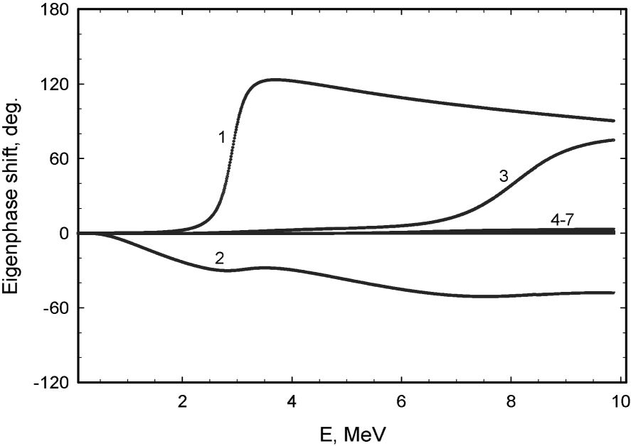
Figure 1: Eigenphase shifts for the $L^{\pi}=1^{-}$, $S=1$ state of ${}^{4}Li$ obtained with the Minnesota potential and $K_{max}=11$. The eigenchannels are numerated.

of so-called 3$\Rightarrow$3 scattering for $L^{\pi}=1^{-}$, $S=1$ state in the ${}^{4}Li$, obtained with the Minnesota potential. Similar pictures are obtained for other nuclei and different ($L^{\pi}$, $S$) states and also with the MHN potential. One can see from Fig. 1 that there are two resonance states in ${}^{4}Li$, first resonance is narrow and manifest itself through the first eigenchannel, while the second resonance is very broad and appear in the third eigenchannel.

The eigenphase shifts provide with a direct and simple way to determine the energy and width of a resonance state in the three-cluster continuum, but to get information concerning the main features of the three-cluster dynamics one needs to analyze the phase shifts $\delta_{ij}$ and the inelastic parameters $\eta_{ij}$.

In Figs. 2 and 3 we display the phase

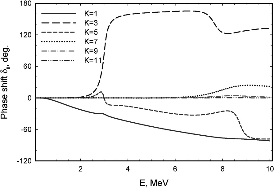
Figure 2: Phase shifts of the 3$\Rightarrow$3 scattering for the $L^{\pi}=1^{-}$, $S=1$ state of ${}^{4}Li$. Results are obtained with the Minnesota potential and $K_{max}=11$.

shifts $\delta_{ii}$ and inelastic parameters $\eta_{ii}$

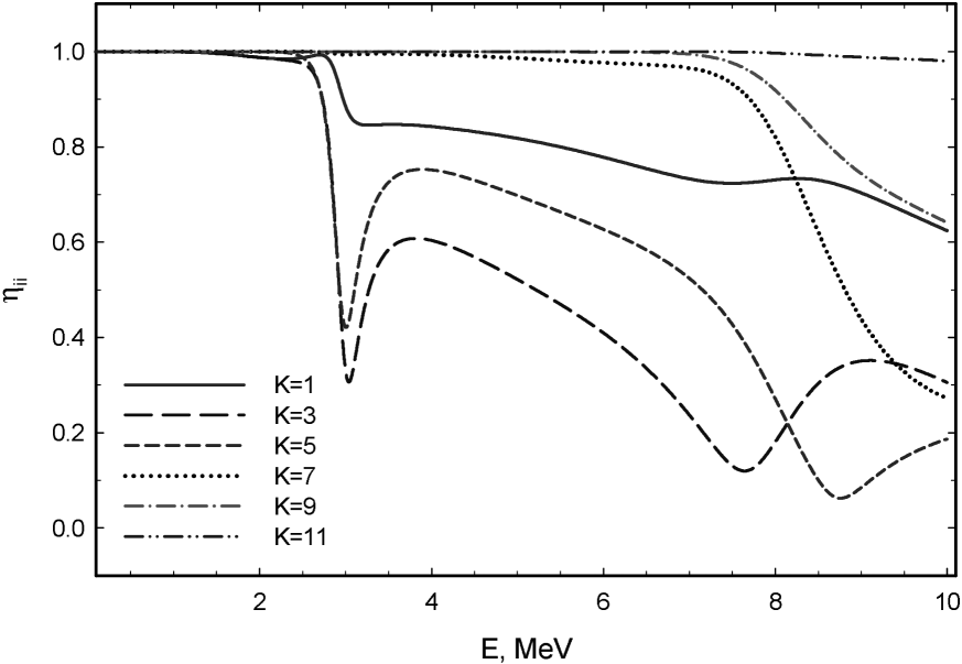
Figure 3: Inelastic parameters of the 3$\Rightarrow$3 scattering for the $L^{\pi}=1^{-}$, $S=1$ state in ${}^{4}Li$. Results are obtained with the Minnesota potential and $K_{max}=11$.

connected with the diagonal matrix elements of the original $S$-matrix. They are obtained for ${}^{4}Li$ and with MP. One notices that only two hyperspherical harmonics are responsible for the lowest $1^{-}$ resonance state. The $K=3$ phase shift displays the classical behavior for a resonance state, while the $K=5$ phase shift indicates a “shadow” resonance. Many more hyperspherical momenta are involved in creating the second resonance.

In Tables 1 and 2 we collect the parameters of the resonance states lying above the three-cluster threshold $d+N+N$. The even parity states are obtained with $K_{\max}=10$, and the odd parity states with $K_{\max}=11$.

Nucleus	$L^{\pi}$	$S$	$K_{\max}$	$E$, MeV	$\Gamma$, MeV	$E$, MeV	$\Gamma$, MeV
${}^{4}H$	$1^{-}$	0	11	1.642	0.367	6.726	2.759
${}^{4}H$	$1^{-}$	1	11	1.911	0.374	6.958	2.982
${}^{4}Li$	$1^{-}$	0	11	2.604	0.413	7.787	3.141
${}^{4}Li$	$1^{-}$	1	11	2.912	0.465	8.085	3.384
${}^{4}He$	$2^{+}$	0	10	1.950	0.233	2.904	0.207

Table 1: Resonance states of ${}^{4}H$, ${}^{4}He$ and ${}^{4}Li$, created by the three-cluster channel $d+N+N$. Results are obtained with the Minnesota potential.

Nucleus	$L^{\pi}$	$S$	$K_{\max}$	$E$, MeV	$\Gamma$, MeV	$E$, MeV	$\Gamma$, MeV
${}^{4}H$	$1^{-}$	0	11	3.972	1.170	9.469	3.440
${}^{4}H$	$1^{-}$	1	11	3.738	0.950	9.250	3.362
${}^{4}Li$	$1^{-}$	0	11	0.748	0.093	5.009	1.531
${}^{4}Li$	$1^{-}$	1	11	0.662	0.056	4.772	1.329
${}^{4}He$	$2^{+}$	0	10	0.890	0.005	2.436	0.167

Table 2: Resonance states of ${}^{4}H$, ${}^{4}He$ and ${}^{4}Li$, created by the three-cluster channel $d+N+N$. Results are obtained with the MHN potential.

It is known that there is an effective barrier in each channel of three-cluster system. The barrier is created by a potential well, resulted from a NN-interaction between nucleons from different clusters, and centrifugal barrier, which is proportional to

$$\frac{\hbar^{2}}{2m}\frac{K(K+4)}{\rho^{2}}$$

In ${}^{4}He$ and ${}^{4}Li$ the Coulomb repulsion

$$\frac{Z_{eff}}{\rho}$$

have to be added to the effective barrier. The effective charge $Z_{eff}$ depends on quantum numbers $\alpha$, $K$, $l_{1}$, $l_{2}$ and its definition can be found in [16]. The deeper is potential well, the larger is the effective barrier and, consequently, more resonance states can be created by such effective barrier. One can see that the effective barrier, generated by the MHN potential, is more deeper than the one connected with the Minnesota potential. As a result of this difference, the resonance states in ${}^{4}H$, obtained with the MHN potential, have larger energy then resonances, calculated with the Minnesota potential.

As we pointed out the results, presented in Tables 1 and 2, for the even parity states are obtained with $K_{\max}=10$, and for the odd parity states with $K_{\max}=11$. These values for $K_{\max}$ are sufficient to obtain stable results. This is demonstrated in Fig. 4

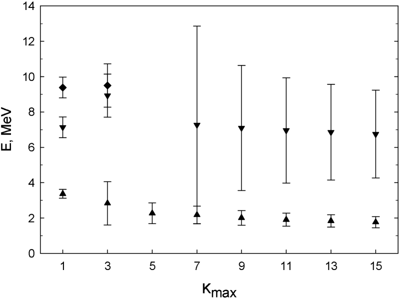
Figure 4: Energy of the $1^{-}$ resonance state of ${}^{4}H$ (total spin $S=1$) as a function of $K_{max}$. Error bars indicate the double of the resonance width. The calculations have been performed with the Minnesota potential.

where the parameters (energy and width) of the $1^{-}$ resonance in ${}^{4}H$ are displayed as a function of $K_{\max}$. The results in Fig. 4 are presented for the Minnesota potential, and similar results are obtained for the MHN potential. We indicate some “false” resonances states appearing at small values of $K_{\max}$ due to the restriction on decay channels compatible with this $K_{\max}$. When we increase the number of open channels, the “false” resonances disappear and the physical resonances converge to their correct positions.

There are some arguments that the physical resonances do not depends on the boundary conditions implemented, or on the used approximations. One can e.g. study the behavior of the so-called Harris states, i.e. the eigenvalues of the Hamiltonian as a function of the number of basis functions involved in a calculation. It was shown (see, for instance, [27, 28]) that the eigenvalues $E_{\nu}\left(n\right)$ ($E_{\nu}\left(n\right)$ is $\nu$-th eigenvalue, obtained with $n$ basis functions) create plateaus at the energies of resonance states. For a very narrow resonance this plateau is already observed for a small value of $n$. For wider resonances, one needs more basis functions to reach a plateau. For a small number of basis functions a wider resonance can become apparent as the repulsion of two eigenvalues (avoided crossing of two eigenvalues). Such behavior of these eigenvalues was observed for the Hamiltonian of the three-cluster configuration $d+N+N$ in ${}^{4}H$, ${}^{4}He$ and ${}^{4}Li$.

4 Conclusion

A microscopic model is formulated to treat properly the two- and three-body boundary conditions. For this aim the Faddeev component is used. The hyperspherical harmonics are used to numerate three-cluster channels. They are very valuable for describing three-cluster asymptotic. Two NN-potentials are involved in the calculations in order to evaluate the sensitivity of the final results with respect to this important factor of a microscopic model.

The model is applied for studying resonances states in ${}^{4}H$, ${}^{4}He$ and ${}^{4}Li$ nuclei, created by the three-cluster configuration $d+N+N$. The results presented here demonstrate that the three cluster configuration creates an effective centrifugal barrier which allows to accommodate several resonances. The effect of the two-cluster channels on the position and width of the three-cluster resonances will be discussed in future work.

5 Acknowledgments

One of the authors (V. V.) gratefully acknowledges the University of Antwerp (RUCA) for a “RAFO-gastprofessoraat 2002-2003” and the kind hospitality of the members of the research group “Computational Modeling and Programing” of the Department of “Mathematics and Computer Sciences”, University of Antwerp, RUCA, Belgium.

References

- [1] Tilley D. R., Weller H. R., and Hale G. M.//Nucl. Phys.–1992.–A541–P.1.
- [2] Viviani M., Kievsky A., Rosati S., George E. A., and Knutson L. D.//Phys.Rev.Lett.–2001.–86–P.3739.
- [3] Viviani M.//Nucl.Phys.–2001.–A689–P.308.
- [4] Filikhin I. N. and Yakovlev S. L.//Yad.Fiz. (Phys.Atomic Nuclei)–2000.–63–P.79(69).
- [5] Carbonell J.//Nucl.Phys.–2001.–A684–P.218–226.
- [6] Carbonell J.//Few Body Syst.Suppl.–2000.–12–P.439–444.
- [7] Kaneko T. and Tang Y. C.//Prog.Theor.Phys.–2002.–107–P.833.
- [8] Pfitzinger B., Hofmann H. M., and Hale G. M.//Phys.Rev.–2001.–C64–P.044003.
- [9] Kanada H., Kaneko T., and Tang Y. C.//Phys. Rev.–1991.–C43– P.371–378.
- [10] Kaneko T. and Tang Y. C.//Progress of Theoretical Physics–2002.–107–P.833–837.
- [11] Vasilevsky V. S., Kovalenko T. P., and Filippov G. F.//Yad.Fiz.–1988.–48–P.217–223(346–357).
- [12] Vasilevsky V. S., Rybkin I. Yu., and Filippov G. F.//Yad.Fiz.–1990.–51–P.71–77(112–123).
- [13] Hofmann M. and Hale G. M.//Nucl.Phys.–1997.–A613–P.69.
- [14] Vasilevsky V. S., Nesterov A. V., Arickx F., and Leuven P. V.//Phys. Atomic Nucl.–1997.–60–P. 343–349.
- [15] Arickx F., Leuven P. V., Vasilevsky V., and Nesterov A. Proc. of the 5th. Int. Spring Seminar in Nuclear Physics.–Singapore: World Scientific Publ., 1995.
- [16] Vasilevsky V. S., Nesterov A. V., Arickx F., and Broeckhove J.//Phys. Rev.–2001.–C63–P. 034606.
- [17] Vasilevsky V. S., Nesterov A. V., Arickx F., and Broeckhove J.//Phys. Rev.–2001.–C63–P. 034607.
- [18] Vasilevsky V. S., Nesterov A. V., Arickx F., and Broeckhove J.//Phys. Rev.–2001.–C63–P.064604.
- [19] Vasilevsky V. S., Nesterov A. V., and Chernov O.//Phys.Atom.Nucl.(Yad.Fiz.)–2001.–64, N8–P.1409–1415(1486–1492).
- [20] Filippov G. F. and Okhrimenko I. P.//Sov. J. Nucl. Phys.–1981.–32–P. 480.
- [21] Filippov G. F.//Sov. J. Nucl. Phys.–1981.–33–p. 488.
- [22] B.V.Danilin and M.V.Zhukov//Yad. Fiz. (Phys. Atomic Nuclei)–1993.–56–P. 67 (460).
- [23] Cobis A., Fedorov D. V., and Jensen A. S.//Phys. Rev.–1998.–C58–P.1403–1421.
- [24] Thompson D. R., LeMere M., and Tang Y. C.//Nucl. Phys.–1977.–A268–P. 53–66.
- [25] Hasegawa A. and Nagata S.//Prog. Theor. Phys.–1971.–45–P.1786–1807.
- [26] F. Tanabe, A. Tohsaki, and R. Tamagaki//Prog. Theor. Phys.–1975.–53–P.677–691.
- [27] Filippov G. F., Vasilevsky V. S., and Chopovsky L. L.//Soviet Journal of Particles and Nuclei(Element.Chast.Atom.Yadra)–1985.–16–P.153–177(349–406).
- [28] Ho Y. K.//Phys. Rep.–1993.–99–P. 1–68.