High-$K$ Precession modes: Axially symmetric limit of wobbling motion

Abstract

The rotational band built on the high-$K$ multi-quasiparticle state can be interpreted as a multi-phonon band of the precession mode, which represents the precessional rotation about the axis perpendicular to the direction of the intrinsic angular momentum. By using the axially symmetric limit of the random-phase-approximation (RPA) formalism developed for the nuclear wobbling motion, we study the properties of the precession modes in ¹⁷⁸W; the excitation energies, $B(E2)$ and $B(M1)$ values. We show that the excitations of such a specific type of rotation can be well described by the RPA formalism, which gives a new insight to understand the wobbling motion in the triaxial superdeformed nuclei from a microscopic view point.

I Introduction

Rotation is one of typical collective motions in atomic nuclei. It manifests itself as a rotational band, a sequence of states connected by strong electromagnetic (e.g. $E2$)-transitions. Most of the rotational bands observed so far are based on the uniform rotation about an axis perpendicular to the symmetry axis of axially symmetric deformation. The well known ground state rotational bands and the superdeformed rotational bands with axis ratio about 2:1 are typical examples of this type of rotational motion. Quite recently, exotic rotational motions, in contrast to the normal ones mentioned above, have been issues under discussion, which are generally non-uniform nor rotating about one of three principal axes of deformation, and clearly indicate possible existence of three-dimensional rotations in atomic nuclei. The recently observed wobbling rotational bands S. W. Ødegård et al. (2001); D. R. Jensen et al. (2002a, b); I. Hamamoto (2002); I. Hamamoto and G. B. Hagemann (2003) and the chiral rotation/vibration bands Frauendorf and Meng (1997); K. Starosta et al. (2001); T. Koike et al. (2003, 2004) are such examples.

Such exotic rotations are very interesting because they give hints to a fundamental question: How does an atomic nucleus rotate as a three-dimensional object? They may also shed light on collective motions in nuclei with triaxial deformation, which are characteristic in these rotational bands, and are very scarce near the ground state region. Although the triaxial deformation is crucial for those exotic rotations, it is not a necessary condition for three-dimensional rotations to occur. For example, the chiral rotation is a kind of “magnetic rotation” or “tilted axis rotation” Frauendorf (2001), where the axis of rotation is neither along a principal axis of deformation nor in the plane of two principal axes, but is pointing inside a triangle composed of three principal axes. In the case of the typical magnetic rotation observed in the Pb region, the so-called “shears band” Frauendorf (2001), the deformation is axially symmetric and of weakly oblate. Similarly, one can think of an axially symmetric limit of the wobbling motion; the so-called “precession band”, which is nothing else but a rotational band excited on a high-$K$ isomeric state, in analogy to the classical motion of the symmetric top. The main purpose of the present paper is to investigate the precession band from a microscopic view point.

In recent publications Matsuzaki et al. (2002, 2004), we have studied the nuclear wobbling motions associated with the triaxial superdeformed (TSD) bands in Lu and Hf isotopes on the basis of the microscopic framework; the cranked mean-field and the random phase approximation (RPA) Marshalek (1977, 1979); Janssen and I. N. Mikhailov (1979); J. L. Egido et al. (1980); Zelevinsky (1980); Y. R. Shimizu and K. Matsuyanagi (1983); Y. R. Shimizu and Matsuzaki (1995). It has been found that RPA eigen-modes, which can be interpreted as the wobbling motions, appear naturally if appropriate mean-field parameters are chosen. The deformation of the mean-field is large ($\epsilon_{2}>0.35$) with a positive triaxial shape ($\gamma\approx+20^{\circ}$ in the Lund convention), i.e., mainly rotating about the shortest axis, and the static pairing is small (${\mit\Delta}_{n,p}<0.6$ MeV), both of which are in accordance with the potential energy surface calculation Bengtsson . It should be stressed that the solution of the RPA eigen-value is uniquely determined, once the mean-field is fixed, as long as the “minimal coupling” residual interaction is adopted (see Sec. III). Therefore, it is highly non-trivial that we could obtain wobbling-like RPA solutions at correct excitation energies. However, the detailed rotational frequency dependence of the observed excitation energy in Lu isotopes, monotonically decreasing with frequency, could not be reproduced, and the out-of-band $B(E2)$ values from the wobbling band were considerably underestimated in our RPA calculation.

By restricting to the axially symmetric deformation with an uniform rotation about a principal axis, the angular momentum of high-spin states is built up either by a collective rotation, i.e., the rotation axis is perpendicular to the symmetry axis, or by alignments of single-particle angular momenta, i.e., the rotation axis is the same as the symmetry axis. Thus, four rotation schemes are possible; oblate non-collective, prolate collective, oblate collective, and prolate non-collective rotations, corresponding to the triaxiality parameter $\gamma=60^{\circ}$, $\gamma=0^{\circ}$, $\gamma=-60^{\circ}$, and $\gamma=-120^{\circ}$ in the Lund convention, respectively. The axially symmetric limit of the RPA wobbling formalism can be taken for the so-called non-collective rotation schemes with oblate or prolate deformation, namely $\gamma=60^{\circ}$ or $\gamma=-120^{\circ}$ cases. In both cases, long-lived isomers are observed, but the rotational bands starting from the isomers have not been observed in the oblate non-collective case. On the other hand, the high-$K$ isomers and the associated rotational bands have been known for many years in the Hf and W region with prolate deformation. Making full use of the axial symmetry, the RPA formalism has been developed Kurasawa (1980, 1982); C. G. Andersson et al. (1981); Skalski (1987), which is capable of describing the rotational band based on the high-$K$ state as a multi-phonon band, i.e., the precession band. Recently, the same kind of rotational bands built on high-$K$ isomers have also been studied by means of the tilted axis cranking model Frauendorf et al. (2000); S. Frauendorf (2000); D. Almehed et al. (2001); S. -I. Ohtsubo and Y. R. Shimizu (2003).

In this paper, we would like to make a link between the two RPA formalisms, those for the (triaxial) wobbling and for the (axially symmetric) precession motions. Moreover, by applying the formalism to the typical nucleus ¹⁷⁸W, where many high-$K$ isomers have been observed, the properties of the precession bands are studied in detail; not only the excitation energies but also the $B(E2)$ and $B(M1)$ values. This kind of study for the precession band sheds a new light on understanding the recently observed wobbling motion. In order to explain the limiting procedure, we review a schematic rotor model in Sec. II, while in Sec. III the RPA wobbling formalism and the connection to the precession band in the axially symmetric limit are considered. The result of calculations for ¹⁷⁸W is presented and discussed in Sec. IV. Sec. V is devoted to some concluding remarks. Preliminary results for the magnetic property of the precession band were already reported Matsuzaki and Shimizu .

II Wobbling and precession in schematic rotor model

The macroscopic rotor model is a basic tool to study the nuclear collective rotation, and its high-spin properties have been investigated within a harmonic approximation Bohr and Mottelson (1975) or by including higher order effects Tanabe and Sugawara-Tanabe (1971); Marshalek (1975); Yamamura (1980). In this section we review the consequences of the simple rotor model according to Ref. Bohr and Mottelson (1975). We use $\hbar=1$ unit throughout in this paper. The Hamiltonian of the simplest triaxial rotor model is given by

$$H_{\rm rot}=\frac{I_{x}^{2}}{2{\cal J}_{x}}+\frac{I_{y}^{2}}{2{\cal J}_{y}}+\frac{I_{z}^{2}}{2{\cal J}_{z}},$$ (1)

where $I$’s are angular momentum operators in the body-fixed coordinate frame, and the three moments of inertia, ${\cal J}_{x}$, ${\cal J}_{y}$ and ${\cal J}_{z}$, are generally different. We assume, for definiteness, the rotor describes the even-even nucleus (integer spins).

Following the argument of Ref. Bohr and Mottelson (1975), let us consider the high-spin limit, $I\gg 1$, and assume that the main rotation is about the $x$-axis, namely the yrast band is generated by a uniform rotation about the $x$-axis. Then, the excited band at spin $I$ can be described by the excitation of the wobbling phonon,

$$X_{\rm wob}^{\dagger}=\frac{a}{\sqrt{2I}}iI_{y}+\frac{b}{\sqrt{2I}}I_{z},$$ (2)

where $a$ and $b$ are the amplitude determined by the eigen-mode equation, $[H_{\rm rot},X_{\rm wob}^{\dagger}]=\omega_{\rm wob}(I)X_{\rm wob}^{\dagger}$, at each spin $I$ in the harmonic approximation. The resultant eigen-value $\omega_{\rm wob}(I)$ is given by the well-known formula,

$$\omega_{\rm wob}(I) = I\sqrt{(1/{\cal J}_{y}-1/{\cal J}_{x})(1/{\cal J}_{z}-1/{\cal J}_{x})}$$ (3)

$$= \omega_{\rm rot}(I)\sqrt{\frac{({\cal J}_{x}-{\cal J}_{y})({\cal J}_{x}-{\cal J}_{z})}{{\cal J}_{y}\,{\cal J}_{z}}},$$ (4)

with the rotational frequency of the main rotation,

$$\omega_{\rm rot}(I)\equiv\frac{I}{{\cal J}_{x}}.$$ (5)

It should be noted that the triaxial deformation of the nuclear shape is directly related to the intrinsic quadrupole moments, e.g. $\tan{\gamma}=-\sqrt{2}Q_{22}/Q_{20}$, but does not give a definite relation between three moments of inertia: One has to introduce a model, e.g. the irrotational flow model, in order to relate the triaxiality parameter $\gamma$ of deformation to three inertia. Actually, if the irrotational moment of inertia is assumed, ${\cal J}_{y}>{\cal J}_{x},{\cal J}_{z}$ for the positive $\gamma$ shape, and then the wobbling frequency (4) becomes imaginary. In our microscopic RPA calculation, the quasiparticle alignments contribute to the ${\cal J}_{x}$ inertia and, as a result, the wobbling mode appears as a real mode even if the mean-field deformation has positive $\gamma$, see Refs. Matsuzaki et al. (2002, 2004) for details.

The spectra of the rotor near the yrast line are given, in the harmonic approximation, by

$$E_{\rm rot}(I,n)=\frac{I(I+1)}{2{\cal J}_{x}}+\omega_{\rm wob}(I)\Bigl{(}n+\frac{1}{2}\Bigr{)},$$ (6)

and are composed of two sequences, the ${\mit\Delta}I=2$ horizontal ones,

$$E^{\rm(hor)}_{n}(I)=E_{\rm rot}(I,n),\quad I=n,n+2,n+4,...$$ (7)

with given phonon numbers $n=0,1,2,...$, and the ${\mit\Delta}I=1$ vertical ones,

$$E^{\rm(ver)}_{I_{0}}(I)=E_{\rm rot}(I,I-I_{0}),\quad I=I_{0},I_{0}+1,I_{0}+2,...$$ (8)

with given band head spins $I_{0}=0,2,4,...$, both of which are connected by $E2$ transitions. The horizontal ones are conventional rotational bands with transition energies $E_{\gamma}\approx 2\omega_{\rm rot}$, and the ${\mit\Delta}I=-2$ in-band $B(E2)$ values are proportional to the square of the quadrupole moment about the $x$-axis. The vertical ones look like phonon bands with transition energies $E_{\gamma}\approx(\omega_{\rm wob}+\omega_{\rm rot})$ and the ${\mit\Delta}I=-1$ vertical $B(E2)$ values are $O(1/I)$ smaller than the horizontal ones. These features are summarized schematically in Fig. 1. In fact, the ${\mit\Delta}I=-1$ out-of-band transition was crucial to identify the wobbling motion in Lu isotopes S. W. Ødegård et al. (2001). If the wobbling-phonon energy $\omega_{\rm wob}(I)$ is larger than the ${\mit\Delta}I=2$ rotational energy ${\mit\Delta}E_{\rm rot}(I)=E_{\rm rot}(I+1,n)-E_{\rm rot}(I-1,n)=(2I+1)/{\cal J}_{x}$, both the ${\mit\Delta}I=\pm 1$ transitions are possible. The ${\mit\Delta}I=-1$ transition is much stronger than the ${\mit\Delta}I=+1$ one for the positive $\gamma$ shape, and vice versa for the negative $\gamma$ shape, which also supports that the TSD bands in the Lu region have positive $\gamma$ shape.

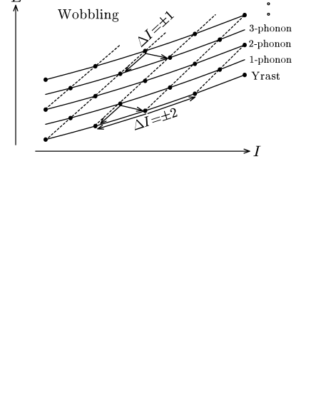
Figure 1: Schematic figure depicting the rotational spectra of a triaxial rotor Hamiltonian. The horizontal rotational bands are connected by solid lines, while the vertical phonon bands by dotted lines.

Now, let us consider the axially symmetric limit Kurasawa (1982). From symmetry argument, without specifying the $\gamma$-dependence of three inertia, if the system is axially symmetric about one of the principal axes, then two inertia about other two axes should coincide. Since the main rotation takes place about the $x$-axis, there are two qualitatively different cases; axially symmetric about the $x$-axis or about the other $y$, $z$-axes. In the latter case, the main rotation is about the axis perpendicular to the symmetry axis like in the case of the ground state rotational band, and then, apparently, the wobbling frequency (4) vanishes; i.e., no wobbling motion takes place. In contrast, if the system is axially symmetric about the main rotation axis $x$, ${\cal J}_{y}={\cal J}_{z}\equiv{\cal J}_{\bot}$, then the wobbling frequency (4) reads

$$\omega_{\rm wob}(I)=\frac{I}{{\cal J}_{\bot}}-\omega_{\rm rot}(I).$$ (9)

Since the vertical transition energy is $\approx\omega_{\rm wob}+\omega_{\rm rot}$, this result means that the slope of the vertical sequence is given by $I/{\cal J}_{\bot}$, while the slope of the horizontal one by $\omega_{\rm rot}=I/{\cal J}_{x}$.

In reality, because the rotor model describes the collective rotation restoring the broken symmetry, ${\cal J}_{x}\rightarrow 0$ (no collective rotation) if the $x$-axis is a symmetry axis. Thus, each horizontal band shrinks to one state, leaving one vertical band, whose transition energy is $I/{\cal J}_{\bot}$. The spin of the starting state $I_{0}=K$ is composed of single-particle alignments, i.e., the band head state is a high-$K$ isomeric state. The precession band is this remaining vertical phonon band, which is actually based on a collective rotation about the perpendicular axis, with large angular momentum $K$ along the symmetry axis. The rotational energy of the band is

$$E_{{\rm high-}K}(I)=\frac{1}{2{\cal J}_{\bot}}[I(I+1)-K^{2}],$$ (10)

which can be rewritten, by putting $I=K+n$, as

$$E_{{\rm high-}K}(I)=\omega_{\rm prec}\left(n+\frac{1}{2}+\frac{n(n+1)}{K}\right),$$ (11)

with

$$\omega_{\rm prec}\equiv\frac{K}{{\cal J}_{\bot}},$$ (12)

leading to a harmonic phonon band structure with a one-phonon energy $\omega_{\rm prec}$, when $K$ is sufficiently large. This precession phonon energy coincides with the vertical transition energy given in Eq. (9) at the band head $I=K$. The spectra in this limit is drawn in Fig. 2. The harmonic picture holds not only for the energy spectra but also for the $B(E2)$ values; for example, by using $B(E2)\propto\langle I_{f}K20|I_{i}K\rangle^{2}$, one finds, in the leading order, $B(E2;n\rightarrow n-1)\propto 3(n/K)$ and $B(E2;n\rightarrow n-2)\propto(3/2)(n(n-1)/K^{2})$, where $n=I-K$ is the number of the precession phonon quanta, so that the two-phonon transition is prohibited when $K$ is large.

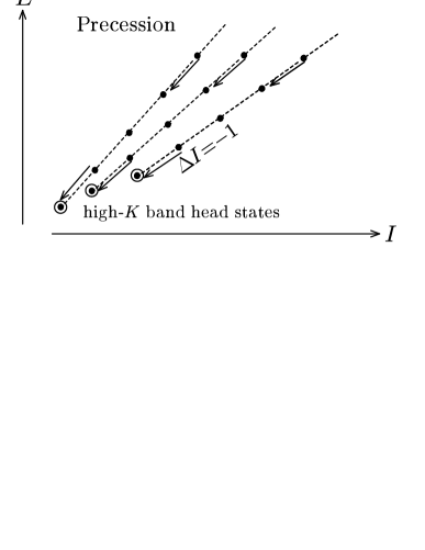
Figure 2: Schematic figure depicting the precession bands excited on high-$K$ isomeric states. Note that the whole $\Delta I=\pm 2$ horizontal sequences shown in Fig. 1 shrink to one such band in the axially symmetric limit.

III Axially symmetric limit of RPA wobbling formalism

III.1 Minimal coupling and RPA wobbling equation

Microscopic RPA theories for nuclear wobbling motion have been developed in Refs. Janssen and I. N. Mikhailov (1979); Marshalek (1979); Zelevinsky (1980). The most important among them is that of Marshalek Marshalek (1979), where the transformation to the principal axis frame (body-fixed frame) is performed and the theory is formulated in that frame. Moreover, it is shown that the RPA equation for the wobbling mode can be cast into the same form as Eq. (4) if three moments of inertia are replaced with those appropriately defined in the microscopic framework; we call this equation the wobbling form equation. The adopted microscopic Hamiltonian in Ref. Marshalek (1979) is composed of the spherical mean-field and the quadrupole-quadrupole interaction (with the monopole pairing if necessary). In Ref. Zelevinsky (1980), however, it was pointed out that the RPA equation could not be reduced to the wobbling form equation, if a most general residual interaction is used. A closer look into the argument in Ref. Zelevinsky (1980) shows, however, that the following “minimal coupling”, being used as a residual interaction, leads to the wobbling form equation as the RPA dispersion equation.

In Marshalek’s theory the rotational Nambu-Goldstone (NG) modes (or spurious modes as conventionally called), $J_{y}$ and $J_{z}$, play a crucial role. The RPA guarantees the decoupling of these modes if the selfconsistency of the mean-field is satisfied in the Hartree-Fock sense. In many cases, however, non-selfconsistent mean-fields are necessary; for example, the deformation is more properly determined by the Strutinsky procedure than by the Hartree-Fock calculations with simple interactions, or one wants to study the system by hypothetically changing the mean-field parameters, as has been done in our previous calculations Matsuzaki et al. (2004) for the nuclear wobbling motions. Thus, we consider that the mean-field, $h$, rather than the interaction is given, and look for the residual interaction, $H^{(m)}_{\rm res}$, which fulfills the decoupling condition of the NG modes within the RPA Pyatov and Salamov (1977). The same idea has been formulated in the context of the particle-vibration coupling theory Bohr and Mottelson (1975), where the rotational invariance is restored by considering the coupling resulting from a small rotation about either the $x$, $y$ or $z$-axis. Thus the minimum requirement is what we call the “minimal coupling” given by

$$H^{(m)}_{\rm res}=-\frac{1}{2}\sum_{k,l=x,y,z}\chi_{kl}F_{k}F_{l}.$$ (13)

Here, the Hermitian operator $F_{k}$ and the $3\times 3$ symmetric force-strength matrix $\chi_{kl}$ are defined as

$$F_{k}=i[h,J_{k}],$$ (14)

$$(\chi^{-1})_{kl}=-\langle{\mit\Phi}|[[h,J_{k}],J_{l}]|{\mit\Phi}\rangle.$$ (15)

with the mean-field vacuum state $|{\mit\Phi}\rangle$ (Slater determinant if no pairing is included), on which RPA eigen-modes are created. If the mean-field is given by the unisotropic harmonic oscillator potential, the minimal coupling leads to the doubly-stretched $Q^{\prime\prime}Q^{\prime\prime}$ interaction combined with the Landau prescription Kurasawa (1980); T. Kishimoto et al. (1975); H. Sakamoto and T. Kishimoto (1989); T. Suzuki and D. J. Rowe (1977); E. R. Marshalek (1983, 1984); Y. R. Shimizu and K. Matsuyanagi (1984); Åberg (1985). One has to include the monopole pairing interaction in realistic calculations. It should be stressed that the minimal coupling can be used for any type of mean-fields, e.g. the Woods-Saxon potential.

For the wobbling modes in the yrast region, the mean-field vacuum state $|{\mit\Phi}(\omega_{\rm rot})\rangle$ is obtained as the lowest eigen-state of the cranked mean-field Hamiltonian,

$$h^{\prime}=h-\omega_{\rm rot}J_{x},$$ (16)

as a function of the rotational frequency $\omega_{\rm rot}$. Assuming the signature symmetry (with respect to a $\pi$-rotation about the $x$-axis) of the mean-field and the conventional phase convention that the matrix elements of the single-particle operators $iJ_{y}$ and $J_{z}$ are real in the mean-field basis, it can be shown that the force-strength matrix $\chi_{kl}$ is diagonal. The excitation of the wobbling phonon corresponds to the vertical ${\mit\Delta I}=\pm 1$ transitions in Sec. II, therefore only the part of the RPA equations which transfer the signature quantum number by $\alpha=1$ is relevant; i.e., only $k,l=y,z$ parts of $H^{(m)}_{\rm res}$ in Eq. (13) contribute. It is now straightforward to follow the same procedure as has been done in Ref. Marshalek (1979), but with modification that the quadrupole field of the interaction is replaced with $F_{k}$ in Eq. (13): Then one finds that the same RPA dispersion equation can be derived:

$$(\omega^{2}-\omega_{\mathrm{rot}}^{2})\left|\begin{array}[]{@{\,}cc@{\,}}A_{y}(\omega)&B_{z}(\omega)\\ B_{y}(\omega)&A_{z}(\omega)\end{array}\right|=0,$$ (17)

where

$$A_{y}(\omega)=I-\omega_{\rm rot}\mathcal{J}_{y}(\omega)+\omega\mathcal{J}_{yz}(\omega),$$

$$A_{z}(\omega)=I-\omega_{\rm rot}\mathcal{J}_{z}(\omega)+\omega\mathcal{J}_{yz}(\omega),$$

$$B_{y}(\omega)=\omega\mathcal{J}_{y}(\omega)-\omega_{\rm rot}\mathcal{J}_{yz}(\omega),$$

$$B_{z}(\omega)=\omega\mathcal{J}_{z}(\omega)-\omega_{\rm rot}\mathcal{J}_{yz}(\omega),$$ (18)

with the following definitions;

$$I=\langle{\mit\Phi}(\omega_{\rm rot})|J_{x}|{\mit\Phi}(\omega_{\rm rot})\rangle$$

$$\qquad\qquad=\sum_{\mu<\nu}2J_{y}(\mu\nu)J_{z}(\mu\nu),$$

$$\mathcal{J}_{y}(\omega)=\sum_{\mu<\nu}\frac{2E_{\mu\nu}J_{y}(\mu\nu)^{2}}{E_{\mu\nu}^{2}-(\omega)^{2}},$$

$$\mathcal{J}_{z}(\omega)=\sum_{\mu<\nu}\frac{2E_{\mu\nu}J_{z}(\mu\nu)^{2}}{E_{\mu\nu}^{2}-(\omega)^{2}},$$

$$\mathcal{J}_{yz}(\omega)=\sum_{\mu<\nu}\frac{2\omega J_{y}(\mu\nu)J_{z}(\mu\nu)}{E_{\mu\nu}^{2}-(\omega)^{2}}.$$ (19)

In these expressions, $\omega$ is the phonon excitation energy, while $E_{\mu\nu}=E_{\mu}+E_{\nu}$ are two-quasiparticle energies with $\alpha=1$, and $J_{y}(\mu\nu)=\langle\mu\nu|iJ_{y}|{\mit\Phi}\rangle$ ($J_{z}(\mu\nu)=\langle\mu\nu|J_{z}|{\mit\Phi}\rangle$) are two-quasiparticle matrix elements of the operator $iJ_{y}$ ($J_{z}$), which are associated with the vacuum state $|{\mit\Phi}(\omega_{\rm rot})\rangle$ and determined by the mean-field Hamiltonian $h^{\prime}$ in the rotating frame. It is now clear that once the mean-field Hamiltonian is given and the vacuum state $|{\mit\Phi}(\omega_{\rm rot})\rangle$ is obtained, the RPA eigen-modes can be calculated without any ambiguity: This is precisely the consequence of the minimal coupling given by Eq. (13).

The rotational NG mode appears as a decoupled $\omega=\omega_{\rm rot}$ solution in the RPA dispersion equation (17);

$${\mit\Gamma}^{\dagger}=\frac{1}{\sqrt{2I}}(iJ_{y}+J_{z})_{\rm RPA}=\frac{1}{\sqrt{2I}}(iJ_{-})_{\rm RPA},$$ (20)

$$J_{\pm}\equiv J_{y}\pm iJ_{z},\quad(\mbox{$x$-axis quantization}),$$ (21)

where the subscript _RPA means the two-quasiparticle transfer part (the particle-hole part if no pairing is included) of the operator. Note that it is normalizable, $[{\mit\Gamma},{\mit\Gamma}^{\dagger}]_{\rm RPA}=1$, because $\langle{\mit\Phi}|[J_{z},iJ_{y}]|{\mit\Phi}\rangle=\langle{\mit\Phi}|J_{x}|{\mit\Phi}\rangle=I\neq 0$. The cranked mean-field (16) describes the rotating state, which has an angular momentum vector aligned with the $x$-axis, and this NG mode plays a role to tilt the whole system by changing the $x$ component of the angular momentum by $-1$ unit. The reason why the NG mode has a finite excitation energy is that there is a cranking term in the hamiltonian (16) (the Higgs mechanism).

Finally, it has been shown by Marshalek Marshalek (1979) that the non-NG part of the RPA dispersion equation (17) is reduced to the wobbling form,

$$(\omega)^{2}=(\omega_{\rm rot})^{2}\frac{({\cal J}_{x}-{\cal J}^{\rm(eff)}_{y}(\omega))({\cal J}_{x}-{\cal J}^{\rm(eff)}_{z}(\omega))}{{\cal J}^{\rm(eff)}_{y}(\omega)\,{\cal J}^{\rm(eff)}_{z}(\omega)},$$ (22)

if three moments of inertia are replaced with microscopically defined ones in the following way;

$$\mathcal{J}_{x}=\frac{I}{\omega_{\rm rot}}=\frac{\langle{\mit\Phi}(\omega_{\rm rot})|J_{x}|{\mit\Phi}(\omega_{\rm rot})\rangle}{\omega_{\rm rot}},$$

$$\mathcal{J}^{\rm(eff)}_{y}(\omega)=\mathcal{J}_{y}(\omega)-\mathcal{J}_{yz}(\omega)\frac{A_{y}(\omega)}{B_{z}(\omega)},$$

$$\mathcal{J}^{\rm(eff)}_{z}(\omega)=\mathcal{J}_{z}(\omega)-\mathcal{J}_{yz}(\omega)\frac{A_{z}(\omega)}{B_{y}(\omega)}.$$ (23)

Since the $y$- and $z$-effective inertia are $\omega$-dependent, the equation is non-linear and they are determined only after solving it.

As for the electromagnetic transition probabilities, Marshalek proposed a $1/I$-expansion technique by utilizing the perturbative boson expansion method Marshalek (1977). The ${\mit\Delta}I=\mp 1$ $E2$ and $M1$ vertical transitions from the one-phonon wobbling band to the yrast band, discussed in Sec. II, can be calculated within the RPA, which is the lowest order in $1/I$, as

$$B(E2;I\pm 1\rightarrow I)\approx|\langle{\mit\Phi}|[Q_{2\mp 1},X_{\rm wob}^{\dagger}]|{\mit\Phi}\rangle|^{2},$$ (24)

$$B(M1;I\pm 1\rightarrow I)\approx|\langle{\mit\Phi}|[\mu_{1\mp 1},X_{\rm wob}^{\dagger}]|{\mit\Phi}\rangle|^{2},$$ (25)

where $X_{\rm wob}^{\dagger}$ is the wobbling phonon creation operator, and the $E2$ and $M1$ operators quantized with respect to the $x$-axis,

$$Q_{2\pm 1}=\frac{i}{\sqrt{2}}(Q_{21}^{(-)}\pm Q_{22}^{(-)}),$$ (26)

$$\mu_{1\pm 1}=\pm\frac{i}{\sqrt{2}}(i\mu_{y}\mp\mu_{z}),$$ (27)

are introduced (see also Ref. Y. R. Shimizu and Matsuzaki (1995)). Here $Q_{2K}^{(\pm)}$ ($K=0,1,2$) are electric quadrupole operators ($z$-axis quantization) with a good signature,

$$Q_{21}^{(-)} = -\sqrt{\frac{15}{4\pi}}\,e\sum_{a=1}^{Z}(xz)_{a}^{(\pi)},$$ (28)

$$Q_{22}^{(-)} = i\sqrt{\frac{15}{4\pi}}\,e\sum_{a=1}^{Z}(xy)_{a}^{(\pi)},$$ (29)

and $\mu_{k}$ ($k=x,y,z$) are magnetic dipole operators,

$$\mu_{k}=\sqrt{\frac{3}{4\pi}}\,\mu_{N}\sum_{a=1}^{A}(g_{l}^{(\tau)}l_{k}+g_{s}^{(\tau)}s_{k})_{a},\quad(\tau=\pi,\nu).$$ (30)

III.2 Axially symmetric limit and RPA precession equation

If the deformation is axially symmetric about the $x$-axis, the angular momentum is generated not by the collective rotation, but by the alignment of the angular momenta of quasiparticles along the symmetry axis. The mean-field vacuum state $|{\mit\Phi}\rangle$, a high-$K$ state, is a multiple quasiparticle excited state, and its spin value is the sum of the projections, ${\mit\Omega}_{\mu}$, of their angular momenta on the symmetry axis; $I=K=\sum_{\mu}^{({\rm occ})}{\mit\Omega}_{\mu}$, i.e., the time reversal invariance is spontaneously broken in $|{\mit\Phi}\rangle$. In this case, the cranking term in Eq. (16) does not change the vacuum state $|{\mit\Phi}\rangle$, so that the rotational frequency $\omega_{\rm rot}$ is a redundant variable: All observables should not depend on $\omega_{\rm rot}$. It is reflected in the fact that the quasiparticle energies linearly depend on the rotational frequency:

$$E_{\mu}(\omega_{\rm rot})=E^{0}_{\mu}-\omega_{\rm rot}{\mit\Omega}_{\mu},$$ (31)

where $E^{0}_{\mu}$ are quasiparticle energies for the non-cranked mean-field Hamiltonian $h$. Since the eigen-value of $J_{x}$, ${\mit\Omega}$, is a good quantum number, it is convenient to rewrite the RPA dispersion equation (17) in terms of the matrix elements of $J_{\pm}$ rather than $iJ_{y}$ and $J_{z}$: After a little algebra, the equation decouples into two equations,

$$(\omega\pm\omega_{\rm rot})\,S_{\pm 1}(\omega\pm\omega_{\rm rot})=0,$$ (32)

where the functions $S_{\rho}(\omega)$ with $\rho=\pm 1$ determine the ${\mit\Delta\Omega}=\pm 1$ solutions, respectively, and are given by

$$S_{\pm 1}(\omega)=\frac{1}{2}\sum_{\mu<\nu}\left\{\frac{(E_{\mu\nu}\pm\omega_{\rm rot})|J_{\pm}(\mu\nu)|^{2}}{E_{\mu\nu}\pm\omega_{\rm rot}-\omega}\right.\qquad\qquad\qquad$$

$$\qquad\qquad\qquad-\left.\frac{(E_{\mu\nu}\mp\omega_{\rm rot})|J_{\mp}(\mu\nu)|^{2}}{E_{\mu\nu}\mp\omega_{\rm rot}+\omega}\right\}.$$ (33)

The precession is a ${\mit\Delta\Omega}=+1$ mode, as is clear from the rotor model in Sec. II, and then only the ${\mit\Delta}I=-1$ $E2$ and $M1$ transitions are allowed; i.e., their ${\mit\Delta}I=+1$ probabilities vanish in Eqs. (24) and (25) because the two RPA transition amplitudes, $\langle{\mit\Phi}|[Q_{21}^{(-)},X_{\rm wob}^{\dagger}]|{\mit\Phi}\rangle$ and $\langle{\mit\Phi}|[Q_{22}^{(-)},X_{\rm wob}^{\dagger}]|{\mit\Phi}\rangle$, are the same in their absolute value with the opposite sign; a corresponding relation holds for the $M1$ amplitudes.

On the other hand, the $y$- and $z$-inertia are the same due to the axial-symmetry about the $x$-axis, and then, just like Eq. (9), Eq. (22) reduces to

$$\omega=\pm\frac{K}{{\cal J}^{(\rm eff)}_{\bot}(\omega)}\mp\omega_{\rm rot}\quad({\mit\Delta\Omega}=\pm 1),$$ (34)

where $I$=$\langle{\mit\Phi}|J_{x}|{\mit\Phi}\rangle$ is denoted by $K$, and the perpendicular inertia ${\cal J}^{(\rm eff)}_{\bot}(\omega)\equiv{\cal J}^{(\rm eff)}_{y}(\omega)={\cal J}^{(\rm eff)}_{z}(\omega)$ is simply written as

$${\cal J}^{(\rm eff)}_{\bot}(\omega)={\cal J}_{\bot}(\omega)\mp{\cal J}_{yz}(\omega)\quad({\mit\Delta\Omega}=\pm 1),$$ (35)

with ${\cal J}_{\bot}(\omega)\equiv{\cal J}_{y}(\omega)={\cal J}_{z}(\omega)$.

The vibrational treatment of the rotational band built on the high-$K$ isomeric state in terms of the RPA has been done for a harmonic oscillator model in Refs. Kurasawa (1980, 1982), and for realistic nuclei by employing the Nilsson potential in Ref. C. G. Andersson et al. (1981), followed by calculations with the Woods-Saxon potential in Ref. Skalski (1987). The residual interaction adopted in Refs. C. G. Andersson et al. (1981); Skalski (1987) is derived by applying the vibrating potential model of Bohr-Mottelson Bohr and Mottelson (1975) to an infinitesimal rotation about the perpendicular axis, and equivalent to the minimal coupling (13): In the axially symmetric case,

$$H_{\rm int}=-\frac{1}{4}\kappa(F_{+}^{\dagger}F_{+}+F_{-}^{\dagger}F_{-}),$$ (36)

with $F_{\pm}$ being defined by using $J_{\pm}$ in Eq. (21),

$$F_{\pm}=\frac{i}{\kappa}[h,J_{\pm}],\quad\kappa=-\frac{1}{2}\langle{\mit\Phi}|[[h,J_{-}],J_{+}]|{\mit\Phi}\rangle.$$ (37)

Note that the mean-field state $|{\mit\Phi}\rangle$ is now a multi-quasiparticle excited state for the non-cranked mean-field Hamiltonian $h$, and so $\omega_{\rm rot}$ does not appear, although it can be used as the “sloping Fermi surface” to obtain optimal states Andersson et al. (1976): The cranking procedure is totally unnecessary in this approach.

The resultant RPA dispersion equations are given for the parts associated with the fields $F_{\pm}$ separately;

$$\omega\,S_{\pm 1}(\omega)=0,$$ (38)

where the functions $S_{\pm 1}(\omega)$ are defined by

$$S_{\pm 1}(\omega)=\frac{1}{2}\sum_{\mu<\nu}\left\{\frac{E^{0}_{\mu\nu}|J_{\pm}(\mu\nu)|^{2}}{E^{0}_{\mu\nu}-\omega}-\frac{E^{0}_{\mu\nu}|J_{\mp}(\mu\nu)|^{2}}{E^{0}_{\mu\nu}+\omega}\right\},$$ (39)

which turn out to be the same functions as Eq. (33) because of the property (31) of quasiparticle energies in the non-collective rotation scheme. It is worth mentioning $S_{+1}(\omega)=-S_{-1}(-\omega)$, so that ${\mit\Delta\Omega}=-1$ modes are obtained as negative energy solutions of the ${\mit\Delta\Omega}=+1$ dispersion equation and vice versa. For the physical ${\mit\Delta\Omega}=+1$ modes, the eigen-energies of the wobbling dispersion equation (32) and the precession one (38) are related as

$$\omega_{\rm wob}=\omega_{\rm prec}-\omega_{\rm rot}.$$ (40)

By comparing it with Eq. (34), we obtain

$$\omega_{\rm prec}=\frac{K}{{\cal J}^{(\rm eff)}_{\bot}},$$ (41)

with ${\cal J}^{(\rm eff)}_{\bot}$ being written as

$${\cal J}^{(\rm eff)}_{\bot}=\frac{1}{2}\sum_{\mu<\nu}\left\{\frac{|J_{+}(\mu\nu)|^{2}}{E^{0}_{\mu\nu}-\omega_{\rm prec}}+\frac{|J_{-}(\mu\nu)|^{2}}{E^{0}_{\mu\nu}+\omega_{\rm prec}}\right\},$$ (42)

which is the microscopic RPA version of Eq. (12) in Sec. II. This ${\cal J}^{(\rm eff)}_{\bot}$ does not depend on $\omega_{\rm rot}$, while both ${\cal J}_{\bot}={\cal J}_{y}={\cal J}_{z}$ and ${\cal J}_{yz}$ in Eq. (35) do. This result can also be obtained directly from the precession dispersion Eq. (38). Note that the perpendicular inertia (42) reduces to the Inglis cranking inertia (or that of Belyaev if pairing is included) in the adiabatic limit $\omega_{\rm prec}\rightarrow 0$.

The reason why the $\omega_{\rm rot}$-dependent wobbling eigen-energy and the $\omega_{\rm rot}$-independent precession eigen-energy is related in a simple way (40) is that the RPA treatment in Refs. Kurasawa (1980, 1982); C. G. Andersson et al. (1981); Skalski (1987) is formulated in the laboratory frame, while Marshalek’s wobbling theory in the principal axis frame (body-fixed frame). The energies in the laboratory frame, $E^{({\rm L})}$, and in the uniformly rotating frame described by the cranked mean-field, $E^{({\rm UR})}$, are related by $E^{({\rm UR})}=E^{({\rm L})}-{\mit\Omega}\omega_{\rm rot}$ for the state which has a projection, ${\mit\Omega}$, of angular momentum on the rotation axis. Moreover, the energies in the principal axis and the uniformly rotating frames are the same under the small amplitude approximation in the RPA. Thus the difference of phonon energies in (40) comes from the difference of coordinate frames where the two approaches are formulated. The rotational NG mode ${\mit\Gamma}^{\dagger}$ (20), appears at zero energy in the precession dispersion Eq. (38) by the same reason. The transformation between the laboratory and the principal axis frames have been discussed more thoroughly in Refs. Marshalek (1979) and Kurasawa (1982).

As for the electromagnetic transition probabilities in the precession formalism C. G. Andersson et al. (1981); Skalski (1987), the RPA vacuum state $|{\rm RPA}\rangle$ is considered to be a stretched eigen-state of the angular momentum, $|I=K,M=K\rangle$, because ${\mit\Gamma}|{\rm RPA}\rangle=0$ for the NG mode (20) (${\mit\Gamma}\propto(J_{+})_{\rm RPA}$). In the same way, the ${\mit\Delta\Omega}=+1$ one-phonon precession state $X_{\rm prec}^{\dagger}|{\rm RPA}\rangle$ corresponds to $|I=K+1,M=K+1\rangle$, because ${\mit\Gamma}X_{\rm prec}^{\dagger}|{\rm RPA}\rangle=[{\mit\Gamma},X_{\rm prec}^{\dagger}]|{\rm RPA}\rangle=0$. Then, by using the Wigner-Eckart theorem, we obtain, for example,

$$\langle I=K||{\cal M}(E2)||I=K+1\rangle=\sqrt{2K+1}$$

$$\qquad\qquad\qquad\times\frac{\langle{\rm RPA}|Q_{2\,-1}X_{\rm prec}^{\dagger}|{\rm RPA}\rangle}{\langle K+1\,K+1\,2\,-1|K\,K\rangle}.$$ (43)

Thus, by inserting explicit expressions of the Clebsch-Gordan coefficients, one finds

$$B(E2;K+1\rightarrow K)=\frac{K+2}{K}\,|\langle{\mit\Phi}|[Q_{2\,-1},X_{\rm prec}^{\dagger}]|{\mit\Phi}\rangle|^{2},$$ (44)

$$B(M1;K+1\rightarrow K)=|\langle{\mit\Phi}|[\mu_{1\,-1},X_{\rm prec}^{\dagger}]|{\mit\Phi}\rangle|^{2},$$ (45)

which coincide, within the lowest order in $1/K$, with Eqs. (24) and (25) in the wobbling formalism.

IV Result and Discussion

IV.1 Calculation of precession bands in ¹⁷⁸W

Table 1: Configurations assigned for high-$K$ isomers in ¹⁷⁸W C. S. Purry et al. (1995, 1998); D. M. Cullen et al. (1999), which are used in the RPA calculations for the precession bands excited on them. The experimental values of the precession one-phonon energy, $\omega_{\rm prec}^{\rm exp}=E_{K}(I=K+1)-E_{K}(I=K)$, are also tabulated in the last column. The neutron states are 1/2^-[521], 5/2^-[512], 7/2^-[514], 7/2⁺[633], 9/2⁺[624], and 7/2^-a[503]. The proton states are 1/2^-[541], 5/2⁺[402], 7/2⁺[404], 9/2^-[514], and 11/2^-[505]. The bold letters indicate the $h_{9/2}$ proton and the $i_{13/2}$ neutron quasiparticles.

$K^{\pi}$	Neutron configuration	Proton configuration	$\omega_{\rm prec}^{\rm exp}$(keV)
13-	7/2+, 7/2-	5/2+, 7/2+	164
14+	7/2+, 7/2-	5/2+, 9/2-	150
15+	7/2+, 7/2-	7/2+, 9/2-	207
18-	7/2+, 7/2-	1/2-, 5/2+, 7/2+, 9/2-	184
21-	5/2-, 7/2+, 7/2-, 9/2+	5/2+, 9/2-	362
22-	5/2-, 7/2+, 7/2-, 9/2+	7/2+, 9/2-	373
25+	5/2-, 7/2+, 7/2-, 9/2+	1/2-, 5/2+, 7/2+, 9/2-	288
28-	5/2-, 7/2+, 7/2-, 9/2+	1/2-, 7/2+, 9/2-, 11/2-	328
29+	5/2-, 7/2+, 7/2-, 9/2+, 1/2-, 7/2-a	1/2-, 5/2+, 7/2+, 9/2-	437
30+	5/2-, 7/2+, 7/2-, 9/2+	5/2+, 7/2+, 9/2-, 11/2-	559
34+	5/2-, 7/2+, 7/2-, 9/2+, 1/2-, 7/2-a	5/2+, 7/2+, 9/2-, 11/2-	621

In the previous papers Matsuzaki et al. (2002, 2004), we have studied the wobbling motions in the triaxial superdeformed bands in Hf and Lu isotopes. As it is demonstrated in the previous section, the precession mode can be described as an axially symmetric limit of the wobbling formalism. Thus we have performed calculations of the precession bands in ¹⁷⁸W, for which richest experimental information is available C. S. Purry et al. (1995, 1998); D. M. Cullen et al. (1999). Exactly the same wobbling formalism is used, but taking the prolate non-collective limit suitable for high-$K$ isomers, i.e., the triaxiality parameter $\gamma=-120^{\circ}$ in the Lund convention. The first result for this nucleus, concentrating on the magnetic property, was reported already in Ref. Matsuzaki and Shimizu .

The procedure of the calculation is the same as in Refs. Matsuzaki et al. (2002, 2004); Matsuzaki and Shimizu : The standard Nilsson potential Bengtsson and Ragnarsson (1985) is employed as a mean-field with the monopole pairing being included;

$$h=h_{\rm Nils}(\epsilon_{2},\gamma)-\sum_{\tau=\nu,\pi}{\mit\Delta}_{\tau}(P_{\tau}^{\dagger}+P_{\tau})-\sum_{\tau=\nu,\pi}\lambda_{\tau}N_{\tau}.$$ (46)

Here the $\epsilon_{4}$ deformation is neglected and all the mean-field parameters are fixed for simplicity. There are a few refinements of calculation, however: 1) the difference of the oscillator frequencies for neutrons and protons in the Nilsson potential is taken into account, and the correct electric quadrupole operator is used, while $Z/A$ times the mass quadrupole operator was used previously, 2) the model space is fully enlarged; $N_{\rm osc}$=3$-$8 for neutrons and 2$-$7 for protons, which guarantees the NG mode decoupling with sufficient accuracy in numerical calculations. As for the point 1), usually, $Q^{(\pi)}\approx(Z/A)(Q^{(\nu)}+Q^{(\pi)})$ holds for static and RPA transitional quadrupole moments in stable nuclei, and therefore, the simplification in the previous paper was a good approximation. It is, however, found that $Q^{(\pi)}$ is appreciably smaller, by about 4$-$8%, than $(Z/A)(Q^{(\nu)}+Q^{(\pi)})$ in ¹⁷⁸W. Thus, in this paper, we make a more precise calculation using the electric (proton) part of the quadrupole operator.

The calculation is performed for the high-$K$ isomeric configurations listed in Table 1; they cover almost all the multi-quasiparticle states higher than or equal to four (more than or equal to two quasineutrons and two quasiprotons), on which rotational bands are observed. The quadrupole deformation is chosen to be $\epsilon_{2}=0.240$, which reproduces in a rough average the value $Q_{0}=7.0$ b for the configurations in Table 1 assumed in the experimental analyses C. S. Purry et al. (1998); D. M. Cullen et al. (1999). The pairing gap parameters are taken, for simplicity, to be 0.5 MeV for two-quasiparticle configurations, and 0.01 MeV for those with more than or equal to four-quasiparticles, both for neutrons and protons. Chemical potentials $\lambda_{\tau}$ ($\tau=\nu,\pi$) are always adjusted so as to give correct neutron and proton numbers. These mean that the choice of parameters in this work is semi-quantitative. As is explained in detail in Sec. III, the final results do not depend on the cranking frequency $\omega_{\rm rot}$ at all for the non-collective rotation about the $x$-axis. We have confirmed this fact numerically and used $\omega_{\mathrm{rot}}=0.001$ MeV in actual calculations (Note that the wobbling RPA formalism requires a finite rotational frequency in numerical calculations). No effective charge is used for the $E2$ transitions, and $g_{s}^{\mathrm{(eff)}}=0.7g_{s}^{\mathrm{(free)}}$ is used for the $M1$ transitions as usual.

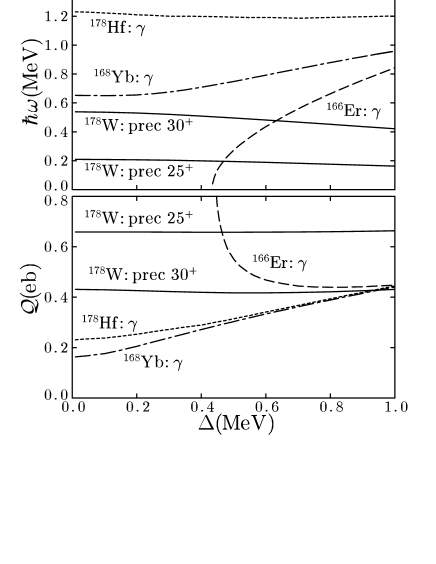
Figure 3: Dependence of numerical results on the pairing gap parameter ${\mit\Delta}={\mit\Delta}_{\pi}={\mit\Delta}_{\nu}$. In the upper panel, the excitation energies are shown, while in the lower panel are shown the RPA transition amplitudes for the electric $Q_{22}^{(-)}$ operator (29). The solid curves show the results for the precession modes excited on the 25⁺ and 30⁺ high-$K$ states in ¹⁷⁸W, and the dotted, dashed and dot-dashed curves represent those for the $\gamma$-vibrations in ¹⁶⁶Er, ¹⁶⁸Yb and ¹⁷⁸Hf, respectively.

Table 2: Mean-field parameters used in the calculation for the $\gamma$-vibrations on the ground states ($\gamma=0^{\circ}$), and observed excitation energies of $\gamma$-vibrations R. B. Firestone et al. (1999). The $\epsilon_{2}$ values are taken from Ref. Löbner et al. (1970), where they are deduced from the measured $B(E2:0^{+}_{g}\rightarrow 2^{+}_{g})$ values. The even-odd mass differences are calculated by the third order difference formula with using the binding energy data in Ref. Audi and Wapstra (1995).

Nucleus	$\epsilon_{2}$	${\mit\Delta_{\nu}}$(MeV)	${\mit\Delta_{\pi}}$(MeV)	$\omega_{\gamma}^{\rm exp}$ (MeV)
166Er	0.272	0.966	0.877	0.786
168Yb	0.258	1.039	0.983	0.984
178Hf	0.227	0.694	0.824	1.175

We have checked the dependences of the results on the variations of the deformation parameter $\epsilon_{2}$ and pairing gaps. Those on the pairing gaps are shown in Fig. 3. In this figure, the excitation energy $\omega$ and the RPA transition amplitude for the electric $Q_{22}^{(-)}$ operator (29), ${\cal Q}\equiv|\langle[Q_{22}^{(-)},X_{\rm prec}^{\dagger}]\rangle|$, which is a measure of the $E2$ collectivity, for the precession modes excited on the $K=25^{+}$ and $K=30^{+}$ configurations, are shown as functions of the pairing gap, ${\mit\Delta}={\mit\Delta}_{\pi}={\mit\Delta}_{\nu}$ (the common value for protons and neutrons). For reference sake, are also included the results for the $\gamma$-vibrations on the ground states, i.e., the ${\mit\Delta}K=\pm 2$ vibrational mode excited on the $\gamma=0^{\circ}$ prolate mean-field (without cranking), for ¹⁶⁶Er, ¹⁶⁸Yb and ¹⁷⁸Hf nuclei. Note that the meaning of the operator $Q_{22}^{(-)}$ is different for $\gamma=-120^{\circ}$ and $\gamma=0^{\circ}$ shapes, so that the comparison of the magnitude of the amplitude ${\cal Q}$ is not meaningful between the precession mode and the $\gamma$-vibrational mode. As it is stressed in Sec. III.1, the precession mode is calculated without any ambiguity once the mean-field is fixed; we have just used the same parameters explained above with an exception that the pairing gaps are varied. The situation for the $\gamma$-vibration is different; one has to include components other than the minimal coupling, (13) or (36). We have used the $K=2$ part of the doubly-stretched $Q^{\prime\prime}Q^{\prime\prime}$ force, and the force strength is determined in such a way that the calculations with adopting the even-odd mass differences as pairing gap parameters reproduce the experimental energies of the $\gamma$-vibration; see Table 2 for the parameters and data used. Then, with the use of the force strength thus fixed, calculations are performed with varying the pairing gaps.

As is clearly seen in Fig. 3, the reduction of pairing gaps makes the excitation energies of $\gamma$-vibration change in various ways depending on the shell structure near the Fermi surface; i.e., the distribution of the ${\mit\Delta\Omega}=\pm 2$ quasiparticle excitations, which have large quadrupole matrix elements. The energy becomes smaller and smaller in the case of ¹⁶⁶Er, and finally leads to an instability ($\omega_{\gamma}\rightarrow 0$); accordingly the transition amplitude ${\cal Q}$ diverges. No instability takes place in the case of ¹⁶⁸Yb and the excitation energy decreases with decreasing ${\mit\Delta}$, while it is almost constant for the $\gamma$-vibration in ¹⁷⁸Hf. However, the transition amplitudes ${\cal Q}$ reduce by about 40$-$60% with decreasing ${\mit\Delta}$ except for ¹⁶⁶Er. These are well-known features for the low-lying collective vibrations; namely, the collectivities of the vibrational mode are sensitive to the pairing correlations; especially enhanced by them. In contrast, for the case of the precession modes, the excitation energies are stable and transition amplitudes are surprisingly constant against the change of the pairing gap. This is a feature common to the wobbling mode excited on the triaxial superdeformed band Matsuzaki et al. (2004). Although both the precession (or the wobbling) and the $\gamma$-vibration are treated as vibrational modes in the RPA, the structures of their vacua are quite different; the time reversal invariance is kept in the ground state while it is spontaneously broken in the high-spin intrinsic states. Since the precession or the wobbling is a part of rotational degrees of freedom, this symmetry-breaking may be an important factor to generate these modes. It should be mentioned that the transition amplitude ${\cal Q}$ for ¹⁶⁶Er leads to about a factor of two larger $B(E2:2^{+}_{\gamma}\rightarrow 0^{+}_{g})$ value than the observed one in the present calculation, in which the model space employed is large enough. The RPA calculation overestimates the $B(E2)$ transition probability for the low-lying $\gamma$-vibration if are used the Nilsson potential as a mean-field and the simple pairing plus $Q^{\prime\prime}Q^{\prime\prime}$ force as a residual interaction T. S. Dumitrescu and I. Hamamoto (1982).

There are many RPA solutions in general, and it is not always guaranteed that the collective solution exists. In some cases collective solutions split into two or more, whose energies are close, and the collectivity is fragmented (the Landau damping), or the character of the collective solution is exchanged. Moreover, in the case of precession-like solutions, the ${\mit\Omega}=\pm 1$ modes interact with each other, as it was shown in Ref. C. G. Andersson et al. (1981). In fact, when the deformation is changed, it is found that the precession mode on the $K^{\pi}=15^{+}$ configuration disappears for $\epsilon_{2}>0.250$, and that on the $K^{\pi}=14^{-}$ splits into two for $\epsilon_{2}>0.245$. Similar situations also occur when changing the pairing gap parameters in a few cases. Apart from these changes, the results are rather stable against the change of the mean-field parameters. The fact that we have been able to obtain collective solutions for all the cases listed in Table 1 indicates that our choice of mean-field parameters are reasonable if not the best.

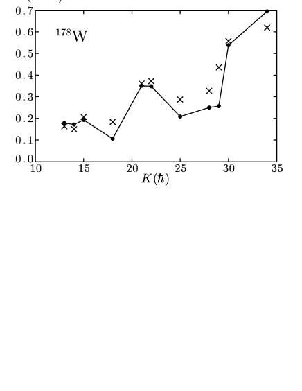
Figure 4: Excitation energies of the one-phonon precession modes excited on high-$K$ configurations. Calculated ones are denoted by filled circles connected by solid lines, and experimental ones by crosses. Data are taken from Refs. C. S. Purry et al. (1998); D. M. Cullen et al. (1999).

Figure 4 presents the calculated and observed relative excitation energies of the first rotational band member, $E_{I=K+1}-E_{I=K}$, i.e., the one-phonon precession energies. Corresponding perpendicular moments of inertia, Eq. (41), are shown in Fig. 5, where the contributions to the inertia from protons and neutrons are also displayed. Our RPA calculation reproduces the observed trend rather well in a wide range of isomeric configurations, from four- to ten-quasiparticle excitations. This is highly non-trivial because, as was stressed in Sec. III, we have no adjustable parameter in the RPA for the calculation of the precession modes once the mean-field vacuum state is given. With a closer look, however, one finds deviations especially at $K^{\pi}=18^{-}$, $25^{+}$, $28^{-}$, and $29^{+}$: The precession energies on them are smaller in comparison with others, but the calculated ones are too small. Low calculated energies correspond to large perpendicular moments of inertia as is clearly seen in Fig. 5. These four configurations contain the proton high-$j$ decoupled orbital (i.e. with ${\mit\Omega}=\pm 1/2$) $\pi$[541]1/2^- originating from the $h_{9/2}$, whose decoupling parameter is large. Occupation of such an orbital makes the Inglis moment of inertia, which is given by Eq. (42) with setting $\omega_{\rm prec}=0$, diverge due to the zero-energy excitation from an occupied ${\mit\Omega}=+1/2$ quasiparticle state to an empty $-1/2$ state. The reason of too large moment of inertia may be overestimation of this effect for the proton contribution in the calculation. The large effect of this $\pi h_{9/2}$ orbital on the moment of inertia has been pointed out also in Refs. Frauendorf et al. (2000); G. D. Dracoulis et al. (1998).

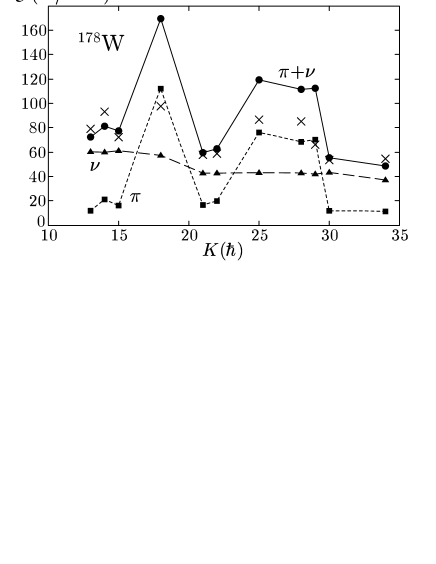
Figure 5: The moment of inertia associated with the precession bands built on high-$K$ configurations. The RPA effective inertia (42) are shown by filled circles connected by solid lines, the proton part of them by filled squares connected by dotted lines, and the neutron part by filled triangles connected by dashed lines. The crosses are those extracted from the experimental spectra according to the simple relation (41).

Except for the case of four configurations including the $\pi$[541]1/2^- orbital, the values of moment of inertia are about 50$-$80 $\hbar^{2}$/MeV, which are smaller than the rigid-body value, ${\cal J}_{\rm rig}$=87.8 $\hbar^{2}$/MeV, and considerably larger than the ground state value, ${\cal J}_{\rm gr}$=28.3 $\hbar^{2}$/MeV. Here ${\cal J}_{\rm rig}$ is calculated by assuming the ¹⁷⁸W nucleus as an ellipsoidal body with $\epsilon_{2}=0.240$ and $r_{0}=1.2$ fm, and ${\cal J}_{\rm gr}$ by $3/E_{2^{+}}$. The pairing gaps are already quenched in the calculation for more than or equal to eight-quasiparticles (four-quasiprotons and four-quasineutrons) configurations ($K\geq 25^{+}$). The value 0.5 MeV of the pairing gap used for two-quasiparticles configurations is already small enough to make the moment of inertia quite large. It is also noticed that the moment of inertia decreases with increasing $K$, which is opposite to the intuition, and clearly indicates the importance of the shell effect for the moment of inertia Deleplanque et al. (2004). In Refs. C. S. Purry et al. (1998); Frauendorf et al. (2000), the angular momentum of the precession band is divided into the collective and aligned ones; the inertia defined in Eq. (41) includes both of them. It is shown that the collective inertia, in which the effect of the aligned angular momentum of the high-$j$ decoupled orbital is removed, takes the value 50$-$60 $\hbar^{2}$/MeV consistent with the other configurations. As is shown in Fig. 5 the proton contribution to the inertia is about 20$-$30% (except for the four configurations above), which is considerably smaller than $Z/A$, but consistent with the calculated value for the $g_{R}$-factor in the ground state rotational band (see below).

As for the electromagnetic transitions in the rotational bands built on high-$K$ isomers, the strong coupling rotational model Bohr and Mottelson (1975) is utilized as a good description. The expressions for $B(E2)$ and $B(M1)$ are well-known:

$$B(E2:I=K+1\rightarrow K)_{\rm rot}\qquad\qquad\qquad\qquad$$

$$=\frac{5}{16\pi}\,e^{2}Q_{0}^{2}\,\langle K+1\,K\,20|KK\rangle^{2}$$ (47)

$$\approx\frac{15}{16\pi}\frac{1}{K}e^{2}Q_{0}^{2},\qquad\qquad$$ (48)

$$B(M1:I=K+1\rightarrow K)_{\rm rot}\qquad\qquad\qquad\qquad$$

$$\quad\qquad=\frac{3}{4\pi}\mu_{N}^{2}\left(g_{K}-g_{R}\right)^{2}K^{2}\,\langle K+1\,K\,10|KK\rangle^{2}$$ (49)

$$\approx\frac{3}{4\pi}\mu_{N}^{2}\left(g_{K}-g_{R}\right)^{2}K,\qquad$$ (50)

where, in the last lines, the Clebsch-Gordan coefficients are replaced with their lowest order expressions in $1/K$. $Q_{0}$ and $(g_{K}-g_{R})$ can be extracted from experiments; the sign of the mixing ratio is necessary to determine the relative sign of them. These quantities are calculated within the mean-field approximation,

$$Q_{0}=\sqrt{\frac{16\pi}{5}}\frac{1}{e}\,\langle Q_{20}\rangle=\Bigl{\langle}\sum_{a=1}^{Z}(2x^{2}-y^{2}-z^{2})_{a}^{(\pi)}\Bigr{\rangle},\qquad$$ (51)

$$g_{K}=\sqrt{\frac{4\pi}{3}}\,\frac{\langle\mu_{x}\rangle}{\mu_{N}\langle J_{x}\rangle},\quad g_{R}=\sqrt{\frac{4\pi}{3}}\,\frac{\langle\mu_{x}\rangle_{\rm gr}}{\mu_{N}\langle J_{x}\rangle_{\rm gr}},$$ (52)

where $\langle\quad\rangle$ means that the expectation value is taken with respect to the high-$K$ configuration ($\gamma=-120^{\circ}$), e.g. $\langle J_{x}\rangle=K$, while $\langle\quad\rangle_{\rm gr}$ with respect to the ground state rotational band ($\gamma=0^{\circ}$). The latter expectation value is calculated by the cranking prescription (16), with the same $\epsilon_{2}$, and with the even-odd mass differences as pairing gaps. The value of $g_{R}$ is thus $\omega_{\rm rot}$-dependent, but its dependence is weak at low frequencies, so that we take the value $g_{R}=0.227$ obtained at $\omega_{\rm rot}\rightarrow 0$, which is much smaller than the standard value, $Z/A=0.416$.

On the other hand, $B(E2)$ and $B(M1)$ are calculated by Eqs. (24) and (25), respectively, in the wobbling formalism which is in the lowest order in $1/K$. By equating these expressions with those of the rotational model, (48) and (50), we define the corresponding quantities in the RPA formalism by ($K=\langle J_{x}\rangle$)

$$(Q_{0})_{\rm RPA}=\sqrt{\frac{16\pi K}{15}}\frac{1}{e}\,\langle[X_{\rm prec}^{\dagger},Q_{2\,-1}]\rangle,$$ (53)

$$(g_{K}-g_{R})_{\rm RPA}=\sqrt{\frac{4\pi}{3K}}\frac{1}{\mu_{N}}\,\langle[X_{\rm prec}^{\dagger},\mu_{1\,-1}]\rangle.$$ (54)

Only their relative phase is meaningful, and the overall phase is chosen in such a way that $(Q_{0})_{\rm RPA}$ is positive. We compare calculated values of $Q_{0}$ in the usual mean-field approximation (51) and in the RPA formalism (53) in Fig. 6 for all high-$K$ configurations listed in Table 1. These two calculated $Q_{0}$’s roughly coincide with each other, but appreciable deviations are seen for the $K^{\pi}=18^{-}$, $25^{+}$, $28^{-}$, and $29^{+}$ isomers: The high-$j$ decoupled orbital $\pi[541]1/2^{-}$ has a large prolate quadrupole moment, so that its occupation generally leads to a larger value of $Q_{0}$. This is clearly seen in Fig. 6 even if $\epsilon_{2}$ is fixed in our calculation. See Ref. F. R. Xu et al. (1998), for example, for the polarization effect of this high-$j$ orbital on $Q_{0}$. It is, however, noticed that the effect is even larger in the RPA calculation just like in the case of the excitation energy in Fig. 4. For the $34^{+}$ isomer we have found a less collective RPA solution at a lower energy, 560 keV, which has about 80% of the $(Q_{0})_{\rm RPA}$ value of the most collective one presented in the figure. The reason why $(Q_{0})_{\rm RPA}$ for the $34^{+}$ isomer is considerably small is traced back to this fragmentation of the precession mode in this particular case. This kind of fragmentation sometimes happens in the RPA calculation.

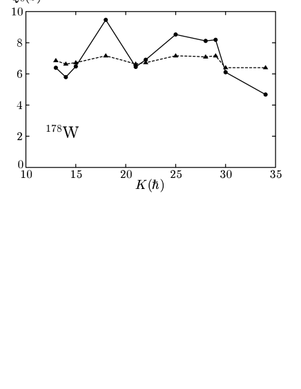
Figure 6: Quadrupole moments $Q_{0}$ for high-$K$ configurations. Those calculated by the RPA, Eq. (53), are denoted by filled circles connected by solid lines, while those by the mean-field approximation, (51), by filled triangles connected by dotted lines.

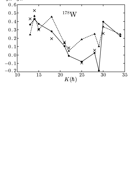
Figure 7: Effective $(g_{K}-g_{R})$-factors for high-$K$ configurations. Those calculated by the RPA, Eq. (54), are denoted by filled circles connected by solid lines, while those by the mean-field approximation (51) by filled triangles connected by dotted lines. Those extracted from the experimental data C. S. Purry et al. (1998); D. M. Cullen et al. (1999) are shown by crosses.

In Fig. 7 we compare the effective $\left(g_{K}-g_{R}\right)$ factors extracted from the experimental data and those calculated in two ways; Eq. (52) and Eq. (54). As for the observed ones they were determined C. S. Purry et al. (1998); D. M. Cullen et al. (1999) from the branching ratios of available lowest transitions in respective rotational bands, by using the rotational model expressions (47) and (49) with $Q_{0}=7.0$ b being assumed. In this way, absolute value $\left|g_{K}-g_{R}\right|$ is obtained, and we assume that its sign is determined by that of the calculated $E2/M1$ mixing ratio in the RPA result. Accordingly, some care is necessary to compare the experimentally extracted $g$-factors with calculations. The agreement between the observed and calculated ones is semi-quantitative, but the RPA result follows the observed trend rather well. Compared to the RPA $g$-factors, those calculated by the mean-field approximation are poorer. Again, the two calculations deviate appreciably for the $K^{\pi}=18^{-}$, $25^{+}$, $28^{-}$, and $29^{+}$ configurations, where the high-$j$ decoupled orbital $\pi[541]1/2^{-}$, which has a large positive $g$-factor, is occupied. The difference between the mean-field $(g_{K}-g_{R})$ and $(g_{K}-g_{R})_{\rm RPA}$ is further discussed in the next subsection by studying the adiabatic limit of the precession mode in the RPA.

IV.2 Interpretation of the result in the adiabatic limit

As it is demonstrated in the previous subsection, the RPA calculation reproduces the precession phonon energies without any kind of adjustments. The electromagnetic properties obtained through the RPA wobbling formalism are in good agreement with those of the strong coupling rotational model, where the quadrupole moments and the effective $g$-factors are calculated within the mean-field approximation. Since the rotational band is described as multi-phonon excitations in the RPA wobbling (or precession) model, it is not apparent that two models lead to similar results for observables. Our results indicate, however, that the RPA treatment of the rotational excitations is valid; especially it gives a reliable microscopic framework for studying the wobbling motion recently observed.

The reason why the RPA precession mode gives the $B(E2)$ and $B(M1)$ similar to those calculated according to the rotational model is inferred by taking the adiabatic limit ($\omega_{\rm prec}\rightarrow 0$) of the RPA phonon creation operator. It has been shown in Ref. Kurasawa (1982) that the precession phonon can be explicitly written up to the first order in $\omega_{\rm prec}$ as

$$X_{\rm prec}^{\dagger} \approx \frac{1}{\sqrt{2K}}(J_{+}+\omega_{\rm prec}{\cal J}_{\bot}^{\rm cr}i{\mit\Theta}_{+})_{\rm RPA}$$ (55)

$$\approx \frac{1}{\sqrt{2K}}(J_{+}+K\,i{\mit\Theta}_{+})_{\rm RPA}.$$

Here the angle operator ${\mit\Theta}_{+}$ is defined by

$${\mit\Theta}_{\pm}={\mit\Theta}_{y}\pm i{\mit\Theta}_{z},$$

$$[h,i{\mit\Theta}_{k}]=\frac{1}{{\cal J}_{\bot}^{\rm cr}}J_{k},\quad(k=y,z),$$ (56)

where ${\cal J}_{\bot}^{\rm cr}$ is the Inglis cranking inertia and given from the effective inertia (42) by setting $\omega_{\rm prec}=0$. These angle operators possess desired properties,

$$\langle[{\mit\Theta}_{k},J_{l}]\rangle=i\delta_{kl}.$$ (57)

For the $E2$ transitions, the contribution of the ${\mit\Theta}_{+}$ part in Eq. (55) is proved to be negligible, if the harmonic oscillator potential is taken as a mean-field;

$$\langle[X_{\rm prec}^{\dagger},Q_{2\,-1}]\rangle\approx\frac{1}{\sqrt{2K}}\langle[J_{+},Q_{2\,-1}]\rangle=\sqrt{\frac{3}{K}}\,\langle Q_{20}\rangle,$$ (58)

which precisely means $Q_{0}\approx(Q_{0})_{\rm RPA}$ in the adiabatic limit.

As for the $M1$ transitions, however, the ${\mit\Theta}_{+}$ part also contributes:

$$\langle[X_{\rm prec}^{\dagger},\mu_{1\,-1}]\rangle\approx\frac{1}{\sqrt{2K}}\Bigl{(}\langle[J_{+},\mu_{1\,-1}]\rangle+K\,\langle[i{\mit\Theta}_{+},\mu_{1\,-1}]\rangle\Bigr{)}$$

$$=\frac{1}{\sqrt{K}}\Bigl{(}\langle\mu_{x}\rangle-\frac{K}{\sqrt{2}}\,\langle[\mu_{1\,-1},i{\mit\Theta}_{+}]\rangle\Bigl{)},$$ (59)

which gives $(g_{K}-g_{R})\approx(g_{K}-g_{R})_{\rm RPA}$ if we identify

$$g_{R}\leftrightarrow{\hat{g}}_{R}\equiv\sqrt{\frac{2\pi}{3}}\frac{1}{\mu_{N}}\,\langle[\mu_{1\,-1},i{\mit\Theta}_{+}]\rangle.$$ (60)

This identification is reasonable: The magnetic moment operator $\mu_{1\,-1}$ possesses a property of angular momentum and is approximately proportional to $J_{-}$. Then the expectation value of the right hand side of Eq. (60) is expected to depend only weakly on the high-$K$ configuration because of Eq. (57). More precisely, if the operators $J_{-}$, ${\mit\Theta}_{+}$ and $\mu_{1\,-1}$ are divided into the neutron and proton parts like

$$J_{-}=J_{-}^{(\pi)}+J_{-}^{(\nu)},\quad{\mit\Theta}_{+}={\mit\Theta}_{+}^{(\pi)}+{\mit\Theta}_{+}^{(\nu)},$$

$$\mu_{1\,-1}\approx\sqrt{\frac{3}{8\pi}}\,\mu_{N}(g^{(\pi)}J_{-}^{(\pi)}+g^{(\nu)}J_{-}^{(\nu)}),$$ (61)

then the following relation is derived,

$${\hat{g}}_{R}\approx\frac{g^{(\pi)}{\cal J}_{\bot}^{{\rm cr}(\pi)}+g^{(\nu)}{\cal J}_{\bot}^{{\rm cr}(\nu)}}{{\cal J}_{\bot}^{{\rm cr}(\pi)}+{\cal J}_{\bot}^{{\rm cr}(\nu)}},$$ (62)

because of $\langle[J_{-}^{(\tau)},i{\mit\Theta}_{+}^{(\tau)}]\rangle=2{\cal J}_{\bot}^{{\rm cr}(\tau)}/{{\cal J}_{\bot}^{\rm cr}}$ with ${\cal J}_{\bot}^{\rm cr}={\cal J}_{\bot}^{{\rm cr}(\pi)}+{\cal J}_{\bot}^{{\rm cr}(\nu)}$ ($\tau=\pi,\nu$). With a cruder estimate $\langle[J_{-}^{(\tau)},i{\mit\Theta}_{+}^{(\tau)}]\rangle\approx 2N_{\tau}/A$ ($\tau=\pi,\nu$), one finds a constant $g_{R}\approx\sum_{\tau}N_{\tau}g^{(\tau)}/A$, which gives a classical result, $Z/A$, by setting $g^{(\pi)}=1$ and $g^{(\nu)}=0$.

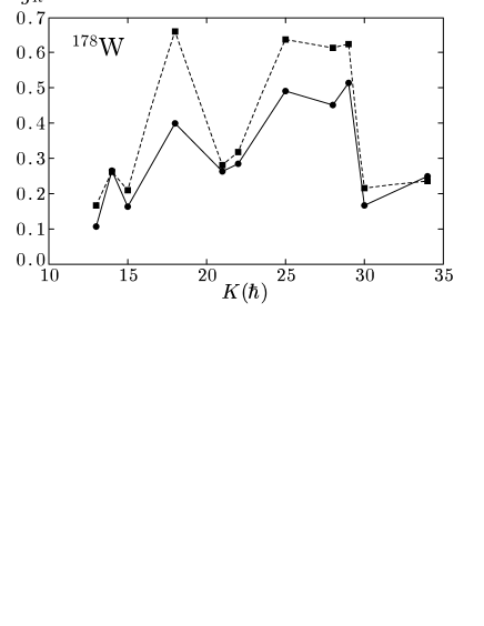
Figure 8: Comparison of deduced $g_{R}$ from two calculations. The one from $g_{K}-(g_{K}-g_{R})_{\rm RPA}$ is denoted by filled circles connected by solid lines, while the quantity ${\cal J}_{\bot}^{({\rm eff},\pi)}/({\cal J}_{\bot}^{({\rm eff},\pi)}+{\cal J}_{\bot}^{({\rm eff},\nu)})$ by filled squares connected by dotted lines.

An approximate relation $g_{R}={\cal J}^{(\pi)}/({\cal J}^{(\pi)}+{\cal J}^{(\nu)})$, which corresponds to Eq. (62) with $g^{(\pi)}=1$ and $g^{(\nu)}=0$, has been used for the ground state rotational band, i.e., the case of collective rotations Bengtsson and Åberg (1986). It seems, however, difficult to justify a similar relation, $g_{R}=Z{\cal J}^{(\pi)}/(Z{\cal J}^{(\nu)}+N{\cal J}^{(\pi)})$, which is used in Ref. C. S. Purry et al. (1998). Thus, the “rotor $g$-factor” $g_{R}$ is not a common constant, but it also depends on the high-$K$ configurations as the intrinsic $g$-factor $g_{K}$ does. In order to see how the approximate relation (62) holds, we compare, in Fig. 8, the two calculated quantities, $g_{K}-(g_{K}-g_{R})_{\rm RPA}$ and ${\cal J}_{\bot}^{({\rm eff},\pi)}/({\cal J}_{\bot}^{({\rm eff},\pi)}+{\cal J}_{\bot}^{({\rm eff},\nu)})$, where the cranking inertia ${\cal J}_{\bot}^{{\rm cr}(\tau)}$, which diverges when the $\pi[541]1/2^{-}$ orbital is occupied, is replaced with the neutron or proton part of the effective inertia (42), see also Fig. 5. As is seen in the figure, these two quantities are in good agreement with each other, again, except for the $K^{\pi}=18^{-}$, $25^{+}$, $28^{-}$, and $29^{+}$ configurations, where the high-$j$ decoupled orbital is occupied and ${\cal J}_{\bot}^{({\rm eff},\pi)}/({\cal J}_{\bot}^{({\rm eff},\pi)}+{\cal J}_{\bot}^{({\rm eff},\nu)})$ is very large. The excitation energies are underestimated for these high-$K$ configurations. Therefore, the proton moments of inertia are overestimated for them; in fact the proton contributions are considerably larger than the neutron ones in these configurations as is shown in Fig. 5. Apart from these four configurations, the deduced $g_{R}$-factors in Fig. 8 are similar to the ground state value, 0.227, though it is appreciably different from the standard value, $Z/A=0.416$. For reference, the cranking moment of inertia for the ground state rotational band calculated using the even-odd mass differences as pairing gaps is ${\cal J}_{\bot}^{\rm cr}=22.7$ $\hbar^{2}$/MeV (about 80% of the experimental value, see the previous subsection). The proton contribution to it is 6.1 $\hbar^{2}$/MeV and ${\cal J}_{\bot}^{({\rm cr})(\pi)}/({\cal J}_{\bot}^{({\rm cr})(\pi)}+{\cal J}_{\bot}^{({\rm cr})(\nu)})=0.269$, which is slightly larger but consistent with the calculated ground state $g_{R}$ value, 0.227.

The above results indicate that the rotor $g_{R}$ should be considered to depend also on the intrinsic configurations, but the dependence is conspicuous only for those including the high-$j$ decoupled orbit, which has a large decoupling parameter as well as a large $g$-factor. The reason why the effective $(g_{K}-g_{R})$-factors of the RPA calculation reproduce the experimentally extracted ones better than those of the mean-field $g$-factors is inferred as follows. Since, as is well known, the $g$-factors of proton orbitals are much larger than those of neutron orbitals, the amount of the proton contribution is overwhelming for the mean-value $\langle\mu_{x}\rangle$ in comparison with that for $\langle J_{x}\rangle$. Considering this fact together with the overestimation of the proton moments of inertia mentioned in the previous paragraph, it is likely that the calculated values of $g_{K}$ (52) for the $K^{\pi}=18^{-}$, $25^{+}$, $28^{-}$, and $29^{+}$ configurations with a proton high-$j$ decoupled orbital are also overestimated. In the mean-field calculation, the calculated values of $(g_{K}-g_{R})$ for those configurations are thus relatively large, because the common ground state $g_{R}$-factor (52) is used. This trend can be seen also in the similar type of mean-field calculations in Refs. C. S. Purry et al. (1998); D. M. Cullen et al. (1999) (Note that different $g_{R}$-factors are used in C. S. Purry et al. (1998) and D. M. Cullen et al. (1999)). In the RPA calculation, however, the rotor $g$-factor is given by ${\hat{g}}_{R}$, (60) or (62), which is overestimated for these four configurations (see Fig. 8). Thus, the overestimation of two $g$-factors may largely cancel out in the resulting $(g_{K}-g_{R})_{\rm RPA}$ values, yielding a reasonable agreement with the experimental data seen in Fig. 7.

The realistic mean-field is not very different from the harmonic oscillator potential so that the approximate equality (58) for the $E2$ operator is expected to hold in general cases. However, it is not very clear to what extent this equality holds: It is a subtle problem whether or not the adiabatic approximation holds because the precession phonon energies are 200 to 600 keV, which are not negligible compared to the quasiparticle excitation energies (Note that the pairing gap is quenched in high-$K$ configurations). In addition to the deviations caused by the non-adiabatic effects, it should also be noticed that the adiabatic approximation itself breaks down if one quasiparticle in a pair of high-$j$ decoupling orbits (${\mit\Omega}_{\mu}=\pm 1/2$) is occupied, because the Inglis cranking moment of inertia diverges due to the zero-denominator. In such cases, the present RPA calculation eventually overestimates the moment of inertia, although it does not diverge. This effect is also reflected in the calculated transition moments $(Q_{0})_{\rm RPA}$ and the effective $g$-factors, which are rather different from the values given by the mean-fields. Whether or not the RPA calculation gives reliable results for such cases, where the non-adiabatic effect is large, is an important future issue. The direct measurement of $Q_{0}$ (i.e. $B(E2)$-value) for the precession band is desirable for this purpose.

V Concluding remarks

We have investigated the precession bands, i.e., the strongly-coupled rotational bands excited on high-$K$ intrinsic configurations by means of the random phase approximation, the microscopic theory for vibrations. It is emphasized that this precession mode is related to the three dimensional motion of the angular momentum vector in the principal axis frame (body-fixed frame), and can be considered to be a limiting mode of the wobbling motion in the triaxially deformed nucleus. It is demonstrated that the observed trend of the precession phonon energies in ¹⁷⁸W is well reproduced by the RPA calculation: This is highly non-trivial because we have employed the minimal coupling interaction, which is determined by the mean-field and the vacuum state based on it, and so there is no adjustable force parameters whatsoever.

The electromagnetic properties, the $E2$ and $M1$ transition probabilities, are also important for this kind of collective excitation modes. We have shown that the calculated $B(E2)$ and $B(M1)$ in terms of the RPA correspond to those given by the conventional rotational model expressions, where the intrinsic quadrupole moment and the effective $g$-factors are calculated within the mean-field approximation. The link between the RPA and the rotational model expressions is given in the adiabatic limit, where the precession phonon energy goes to zero. Then the rotor $g_{R}$-factor is not a common factor any more, but depends on the configurations, especially on the occupation of the high-$j$ decoupled proton orbital. Since the RPA formalism includes this effect properly, the calculated $B(M1)$ values reproduces the experimentally deduced ones rather well. It is, however, noticed that the adiabatic approximation is not necessarily a good approximation because the precession energies are not very small; more crucially, if a high-$j$ decoupled orbital with ${\mit\Omega}=1/2$ is occupied, the approximation breaks down completely. Therefore, it is an important future task to examine how the non adiabatic effect plays a role in the realistic cases. More experimental data, especially $B(E2)$ and $B(M1)$ values, are necessary for this purpose.

Finally, it is worth mentioning the similar RPA calculations for the wobbling motion in the Lu and Hf region. We have presented the result in the recent papers Matsuzaki et al. (2002, 2004). Although we obtained the RPA solutions, which have expected properties of the wobbling motion, the calculated out-of-band over in-band $B(E2)$ ratios were smaller than the measured ones by about a factor two to three; this was the most serious problem in our microscopic calculation. The measured ratio is almost reproduced by the simple rotor model. Both the out-of-band and in-band $B(E2)$, which are vertical and horizontal transition discussed in Sec. II, are expressed in terms of the intrinsic quadrupole moments, $Q_{20}$ and $Q_{22}$ Bohr and Mottelson (1975) (or e.g. deformation parameters ($\epsilon_{2},\gamma$)), combined with the wobbling phonon amplitudes. In the RPA wobbling formalism, on the other hand, the in-band transition is calculated by the intrinsic moments, while the out-of-band transition by the RPA phonon transition in Eq. (24). Thus the underestimation of the $B(E2)$ ratio above means that the RPA phonon transition amplitudes is smaller by about 50$-$70% than the expected ones.

The adiabatic approximation can also be considered for the case of the wobbling phonon Marshalek (1979). Similar correspondence between the intrinsic moments and the RPA transition amplitudes, like $Q_{0}\approx(Q_{0})_{\rm RPA}$ in the present paper, is obtained with a non-trivial modification: There are two amplitudes related to the operators $Q_{21}^{(-)}$ and $Q_{22}^{(-)}$ in Eq. (29), and the $B(E2)$ is calculated by a linear combination of them with coefficients involving the three moments of inertia. Therefore, incorrect coefficients of amplitudes would make $B(E2)$ values to deviate considerably, even though the adiabatic approximation is applicable and two amplitudes are obtained in a good approximation. There is, of course, another possibility that the adiabatic approximation itself is no longer valid. It should be noted that the wobbling excitation energies observed in Lu isotopes are about 200$-$500 keV, which are not small if translated to the transition phonon energy in the laboratory frame, $\omega_{\rm wob}+\omega_{\rm rot}$; see Eq. (40). In the light of the present investigation, it may be possible that the RPA approach yields the correct magnitude of out-of-band transitions also for the case of the wobbling mode, because it actually does in the case of the precession phonon bands. Thus, it is a very important future issue to examine whether or not the RPA wobbling formalism can describe the observed $B(E2)$ ratio in the Lu and Hf region.