Mononuclear caloric curve in a mean field model

Abstract

A mean field model is used to investigate if a plateau in caloric curve can be reached in mononuclear configuration. In the model the configuration will break up into many pieces as the plateau is approached.

The appearence of a plateau in the experimental nuclear caloric curve, since it was pointed out first in [1], has continued to be an important issue in intermediate energy heavy ion collisions [2]. The plateau would signify a maximum in specific heat and could be a signature of a phase transition.

The appearence of a maximum in the specific heat at temperature $T\approx$ 5 MeV was seen in theoretical calculations much earlier [3]. The model is the SMM (Statistical Multifragmentation Model) where it is assumed that the nucleus breaks up into many pieces at a volume significantly larger than the normal nuclear volume. Subsequent modelling has reinforced this picture of a heated nucleus breaking up into pieces as the phenomenon which gives a peak in the specific heat. Take, for example, the LGM (Lattice Gas Model) [4]. Here at low temperature there is a large percolating cluster. As the temperature is raised one reaches a point when the percolating cluster breaks up into many smaller clusters. It is here that the maximum in specific heat is seen (Fig.(19.2) in [2]). This is more dramatically demonstrated in the canoncal thermodynamic model (which is in the same spirit as the SMM but is much easier to implement). Here also at low temperature there is a large blob of matter which breaks up into many pieces and again the maximum in specific heat is obtained in this region. The thermodynamic model can be extrapolated to large numbers of particles. In this limit it is shown that the break up is very sudden as a function of temperature. This is a case of first order phase transition and the maximum of specific heat is obtained at the phase transition.

The present work is inspired by a recent calculation which showed that, in a different model, a plateau in the caloric curve (hence a maximum in specific heat) can be reached in mononuclear configurations as well [5]. One assumes that $e*$(=the excitation energy per particle) as a function of density increases quadratically about the ground state density. At a given excitation energy, the nucleus expands in a self-similar fashion till it reaches its maximum entropy. Effects of interaction on entropy is taken through a parametrisation of $m*/m$ where $m*$ is the effective mass. A temperature is defined microcanonically. The authors then find that when they plot temperature against excitation energy a plateau is found around 5 to 6 MeV.

A more familiar model in nuclear physics which allows study of the caloric curve in mononuclear configurations is the temparature dependent mean field model (Hartee-Fock and/or Thomas-Fermi model). This has certain advantages. When one does a standard mean field calculation at a fixed temparture, one minimises the free energy $F=E-TS$ [6]. This means that when we get the self-consistent solution at a given temperature, we have obtained a solution which has zero pressure. If we draw a caloric curve with energies of these solutions this caloric curve pertains to zero pressure. The specific heat that we will get will be $c_{p}$ with $p=0$.

Investigation of the caloric curve with temperature-dependent Thomas-Fermi theory was done in the past [7]. For nuclei ¹⁵⁰Sm and ⁸⁵Kr caloric curves were drawn and a maximum in specific heat at temperature 10 MeV was found. But there is ambiguity whether the systems stay mononuclear or not. Even though we are interested in finite nuclei, when we do finite temperature mean field theory beyond a certain temperature, fermi occupation factors for orbitals in the continuum will cause the finite system to spread out. The calculations have to be done in a big box and the size of the box will affect the answers. Although given the box, definite numerical results can be obtained it will be hard to decide whether it is a mononucleus or a system of gas. This is best explained using figs. 1 and 2 of [7]. Looking at figures one would venture to say that at temperature 5 MeV we have a mononucleus but at temperature 10 MeV the nucleus spreads to 12.5 fm with density $\approx 0.008fm^{-3}$. Is this a gas or a nuclear liquid?

A much more definite answer can be obtained in the nuclear matter limit. This is pursued in this work. For a fixed temperature we do calculations for different densities. The density where the free energy per particle is minimised is the solution for this temperature; $e*$ of this solution is the appropriate $e*$ for this temperature. As expected, starting from zero temperature, the system expands. The minima of free energy drop to lower and lower density as the temperature increases. But beyond a certain temperature, minimum in free energy disappears. The nucleus will now break apart. This happens before $T$ flattens out as a function of $e*$. This is shown in figs. 1 and 2.

It remains to give some details of the calculation. We use the mometum dependent mean field of [8, 9]. The potential energy density is given by

$$v(\rho)=\frac{A}{2}\frac{\rho^{2}}{\rho_{0}}+\frac{B}{\sigma+1}\frac{\rho^{\sigma+1}}{\rho_{0}^{\sigma}}+\frac{C}{\rho_{0}}\int\int d^{3}pd^{3}p^{\prime}\frac{f(\vec{r},\vec{p})f(\vec{r},\vec{p}^{\prime})}{1+[\frac{\vec{p}-\vec{p}^{\prime}}{\Lambda}]^{2}}$$ (1)

Here $f(\vec{r},\vec{p})$ is phase-space density. In nuclear matter, at zero temperature $f(\vec{r},\vec{p})=\frac{4}{h^{3}}\Theta(p_{F}-p)$ where 4 takes care of spin-isospin degeneracy. At finite temperature the theta function $\Theta(p_{F}-p)$ is replaced by Fermi occupation factor (see details below). The potential felt by a particle is

$$u(\rho,\vec{p})=A[\frac{\rho}{\rho_{0}}]+B[\frac{\rho}{\rho_{0}}]^{\sigma}+2\frac{C}{\rho_{0}}\int d^{3}p^{\prime}\frac{f(\vec{r},\vec{p}^{\prime})}{1+[\frac{\vec{p}-\vec{p}^{\prime}}{\Lambda}]^{2}}$$ (2)

Here $A=$-110.44 Mev, $B$=140.9 MeV, $C$=-64.95 MeV, $\rho_{0}=0.16fm^{-3}$, $\sigma$=1.24 and $\Lambda=1.58p_{F}^{0}$. This gives in nuclear matter binding energy per particle=16 MeV, saturation density $\rho_{0}=.16fm^{-3}$, compressibility $K$=215 MeV and $m*/m$=.67 at the fermi energy; $u(\rho,p)$ gives the correct general behaviour of the real part of the optical potential as a function of incident energy. A comparison of $u(\rho,p)$ with that derived from UV14+UVII potential in cold nuclear matter can be found in [9]. The specific functional form of the momentum dependent part arises from the Fock term of an Yukawa potential. Mean fields given by eqs. (1) and (2) have been widely tested for flow data [10] and give very good agreement.

To do a finite temperature calculation the following steps have to be executed. We need to find the occupation probability

$$n[\epsilon(p)]=\frac{1}{e^{\beta[\epsilon(p)-\mu]}+1}$$ (3)

for a given temperature $1/\beta$ and density $\rho$. If $\epsilon(p)$ were known a priori, this would merely entail finding the chemical potential from

$$\rho=\frac{16\pi}{h^{3}}\int_{0}^{\infty}p^{2}n[\epsilon(p)]dp$$ (4)

But the expression for $\epsilon(p)$ is

$$\epsilon(p)=\frac{p^{2}}{2m}+A[\frac{\rho}{\rho_{0}}]+B[\frac{\rho}{\rho_{0}}]^{\sigma}+R(\rho,p)$$ (5)

where at finite temperature

$$R(\rho,p)=2\frac{C}{\rho_{0}}\frac{4}{h^{3}}\int d^{3}p^{\prime}n[\epsilon(p^{\prime})]\times\frac{1}{1+[\frac{\vec{p}-\vec{p}^{\prime}}{\Lambda}]^{2}}$$ (6)

Thus knowing $R(\rho,p)$ requires knowing $n[\epsilon(p^{\prime})]$ already for all values of $p^{\prime}$. This self-consistency condition can be fulfilled by an iterative procedure (details can be found in [9]).

To calculate pressure, we use the thermodynamic identity $pV=-E+TS+\mu N$ which then gives

$$p=a+b+c$$ (7)

Here

$$a=-v-\frac{16\pi}{h^{3}}\int_{0}^{\infty}dp\frac{p^{4}}{2m}n[\epsilon(p)]$$ (8)

where $v$ is given by eq. (1) and the second term is the contribution from the kinetic energy.

$$b=-T\frac{16\pi}{h^{3}}\int_{0}^{\infty}p^{2}[n\ln n+(1-n)\ln(1-n)]dp$$ (9)

The term $c$ is $\mu\rho$. The free energy per particle is $-(a+b)/\rho$. The test $p=0$ when the minimum of free energy is reached provides a sensible test of numerical accuracy.

A second set of calculation was done with a potential energy density without any momentum dependence. This means the $C$ terms in eqs. (1) and (2) are put to zero and $A,B$ and $\sigma$ are readjusted to give desired values of binding energy per nucleon, equilibrium density and compressibility. The constants now are $A$=-356.8 MeV, $B$=303.9 MeV and $\sigma=$7/6. We study equilibrium values of density with temperature with both the interactions but so, as not to clutter up figures, only the curves with momentum dependent interaction is shown in fig.1. In fig.2 we draw the caloric curves with both sets of interaction and for reference, Fermi gas results $e*=aT^{2}$ are also shown.

In [5], the effects of interactions on the caloric curve were taken through an effective mass $m*$ replacing the real nucleon mass $m$. Normally one writes $m*/m=m_{k}m_{\omega}$. In momentum independent mean field both $m_{k}$ and $m_{w}$ are ignored and $m*/m$=1. In the momentum dependent mean field calculation that we have done here $m_{k}$ is in but $m_{\omega}$ is not. But in both the models, the nucleus will break up before $T$ flattens out against $e*$. As in [5], with momentum dependence the curve is initially above the Fermi gas and meets the Fermi gas curve at some later point.

The mean field model thus reinforces what has long been perceived in other models. At low temperature, the system has a large mass. There are probably some lighter masses too. As the temperature increases the larger mass which has the bulk of the system will break up. This is the point where the caloric curve flattens out. We also note that experimentally the interesting features of the caloric curve occur around 6 MeV temperature whereas in figs 1 and 2 they are occurring around 12 MeV temperature. The finiteness of the system will bring this down as will the Coulomb interaction. In any case some overestimation in mean field theory is expected. In the Ising Model mean field calculations overestimate the critical temperature by fifty per cent [12].

Lastly the lessons from the simple mean field model done here can be used to bolster the expanding emitting source (EES) model of W. Friedman [13]. The model assumes that initially the hot system evaporates as well as expands. For low initial temperature the system will cease expanding and will revert towards normal density. But beyond a certain temperature at the end of this slow expansion the system will explode.

I thank Lee Sobotka for many communications. This work is supported in part by the Natural Sciences and Engineering Research Council of Canada and in part by the Quebec Department of Education.

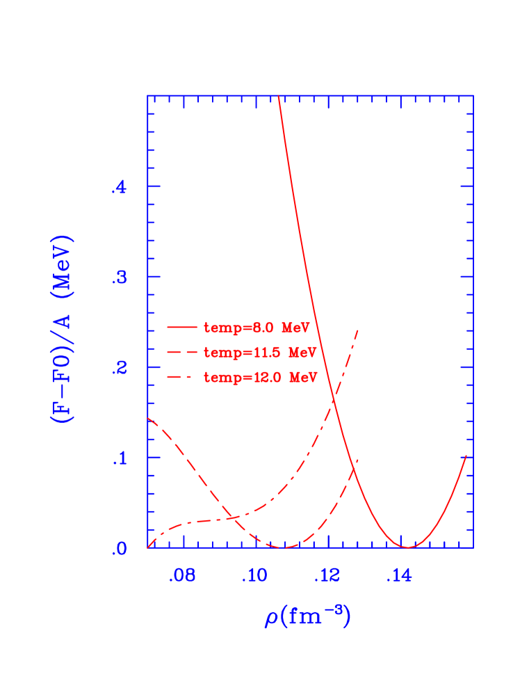
FIG. 1.: The free energy per particle as function of density at different temperatures. This is plotted as a difference from the minimum value of F in the frame. At temperature 12 MeV there is no minimum and the system will roll down to lower density. For this temperature already at lower values of $\rho$ in the figure, the derivative $\frac{\partial p}{\partial\rho}$ is negative, i.e., the system has entered a region of mechanical instability.

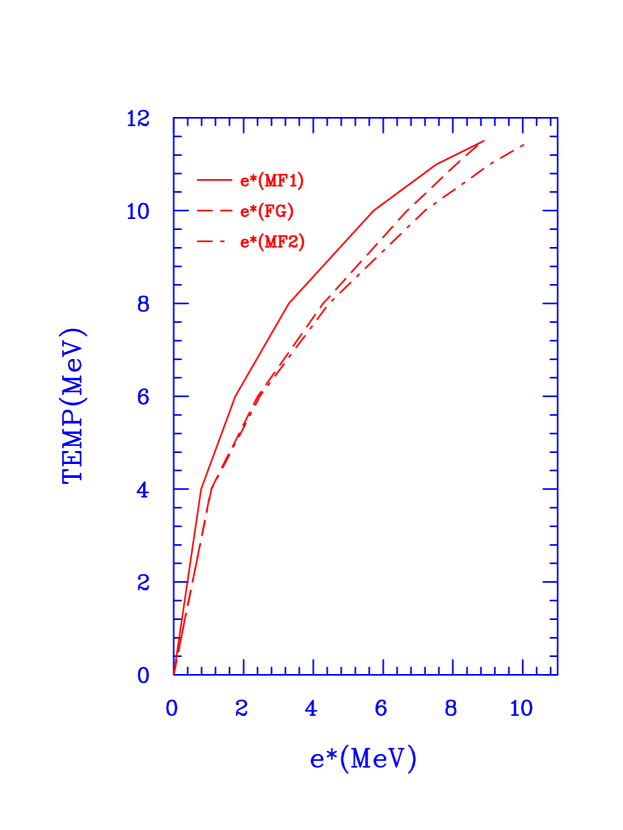
FIG. 2.: Temperature against e* in mean field model with momentum dependence (MF1), in Fermi gas model (FG) and in mean field model without momentum dependence (MF2). As in ref. 5, the curve with momentum dependence lies above the Fermi gas curve till they meet (around temperature 11.5 MeV). The MF1 curve has not yet flattened out. Just below temperature 12 MeV the curve stops. The nucleus will break up into many pieces at higher temperature. Similar situation happens with MF2 except that here it will break up many pieces at $\approx$ 12.5 temperature again before the caloric curve flattens out.

REFERENCES

- [1] J. Pochodzalla et al., Phys. Rev. Lett. 75, 1040 (1995)
- [2] S. Das Gupta, A. Z. Mekjian and M. B. Tsang, Advances in Nuclear Physics, vol.26, 91 (2001)
- [3] J. P. Bondorf, R. Donangelo, I. M. Mishustin, and H. Schulz, Nucl. Phys. A444,321 (1985)
- [4] J. Pan and S. Das Gupta, Phys. Rev. C51 ,1384 (1995)
- [5] L. G. Sobotka, R. J. Charity, J. Toke and W. U. Schroder, Phys. Rev. Lett. 93 ,132702 (2004)
- [6] N. H. March, W. H. Young and S. Sampanther, The Many-Body problem in Quantum Mechanics,(Cambridge University Press, Cambridge, 1967)p. 243
- [7] J. N. De, S. Das Gupta, S. Shlomo, and S. K. Samaddar, Phys. Rev C55,R1641 (1997)
- [8] G. M. Welke, M. Prakash, T.T. S. Kuo, S. Das Gupta, and C. Gale, Phys. Rev. C38, 2101 (1988)
- [9] C. Gale, G. M. Welke, M. Prakash, S. J. Lee and S. Das Gupta, Phys. Rev. C41, 1545 (1990)
- [10] J. Zhang, S. Das Gupta and C. Gale, Phys. Rev. C50, 1617 (1994)
- [11] C. Mahaux, P. F. Bortignon, R. A. Broglia and C. H. Dasso, Phys. Rep. 120, 1 (1985)
- [12] K. Huang, Statistical Machanics(John Wiley and Sons, New York, 1987)Chapter 14
- [13] W. A. Friedman, Phys. Rev. C42, 667 (1990)