Non-perturbative finite $T$ broadening of the $\rho$ meson and dilepton emission in heavy ion-collisions

Abstract

We study self-consistently the finite $T$ broadening of the $\rho$-meson and its implications for dilepton emission in heavy ion-collisions. For this purpose finite width effects at finite temperature due to the $\rho$-$\pi$ interaction are investigated in a self-consistent $\Phi$-functional approach. The temperature dependence of the $\rho$-meson and pion spectral functions and self-energies is discussed. The spectral functions show considerable broadening in comparison with a perturbative calculation on the one-loop level. Using these spectral functions, we make a comparison to dilepton emission data from the CERES NA49 collaboration employing a parametrized fireball evolution model of collision. We demonstrate that these non-perturbative finite width effects are in-medium modifications relevant to the understanding of the enhancement of the low invariant mass spectrum of dileptons emitted in A-A collisions.

I Introduction

In recent years many theoretical and experimental research has been undertaken to investigate the physics of ultra-relativistic heavy-ion collisions (URHIC). The important goal here is to gain a better understanding of the properties of extremely hot and dense nuclear matter. Through variation of the experimental parameters - e.g. collision energy and impact parameter - different regimes of temperature and net-baryon density of the nuclear system are explored. The ultimate goal is to understand the phase structure of quantum chromodynamics (QCD), the theory of strong interactions.

In order to extract reliable information about the properties of nuclear matter under these extreme conditions (and especially to decide if a phase transition from the phase of (confined) hadronic matter to the (partonic) quark-gluon-plasma (QGP) has taken place) one has to do a careful and comprehensive analysis of the experimentally accessible observables. Dileptons ($e^{+}e^{-}$ and $\mu^{+}\mu^{-}$ pairs) and real photons are interesting probes in this context. Since they are emitted during all collision phases and leave the interaction region without substantial rescattering due to the smallness of the electromagnetic coupling. Hence, they reflect the whole space-time evolution of the collision process, in contrast to hadronic probes which predominantly reflect the conditions at kinetic decoupling.

To some degree, measurements made so far complement each other: while photons have been measured for comparative large transverse momentum scales of 1.5 GeV and above, the invariant mass spectrum of dielectrons is rather well known below 1 GeV. Therefore, the measured photons naturally carry information about the early, hard partonic stages of the collision process whereas the scale set by the dilepton measurement dominantly reflect the later, soft hadronic stages.

While there is little reason to assume that low mass dilepton physics would be dominated by emission from a QGP, understanding the late hadronic phase of the evolution is nevertheless of crucial importance for forming a comprehensive picture of the whole collision process. The most intriguing physics question here is the possibility of in-medium modifications of hadron properties. The CERES and HELIOS-3 collaborations demonstrated that central nucleus-nucleus (A-A) collisions exhibit a strong enhancement of low-mass dileptons in the range between $200\text{ MeV}$ and $600\text{ MeV}$ as compared to the yield one expects from the corresponding rates of proton-nucleus (p-A) and proton-proton collisions Masera (1995); Agakishiev et al. (1995, 1998); Lenkeit et al. (1999); Porter et al. (1997); Wilson et al. (1998) which may hint at such modifications. For an overview of the various mechanisms brought forward to explain this enhancement see e.g. Rapp and Wambach (2000).

It is often argued that a large broadening of the $\rho$-meson spectral function cannot be expected by a purely mesonic medium. This assumption is based on perturbative calculations of finite width effects of pions on the $\rho$-meson at finite temperature Gale and Kapusta (1991). However, these investigations consider the width of the $\rho$-meson caused by stable particles only. In most of the theoretical investigations the damping width due to collisional broadening is ignored or investigated in an extended perturbative frameworkUrban et al. (1998). Although investigation of collisional broadening effects due to the interaction of vector mesons with thermal mesons in a kinetic theory framework have been carried out, they consider possible scattering processes of on-shell mesons only Haglin (1995); Gao et al. (1998). In contrast we extend these studies in order to include also off-shell contributions.

In the present paper we study these broadening effects and demonstrate that even the $\pi$ - $\rho$ interaction alone is able to induce substantial broadening of the $\rho$-mesons’s spectral function due to the in-medium damping width of the pion.

For the purpose of studying this mechanism, we employ a many body resummation which is known as the $\Phi$-functional approach. In this approach we derive Dyson Schwinger equations for the propagators of the $\rho$-meson and the pion. Our calculation are self-consistent in the sense that the in-medium broadening of the $\rho$-meson and the pions is taken taken into account by this scheme in its reciprocal dependence.

We concentrate on the phenomenology of collisional broadening and leave the effect of mass shifts relative to the vaccum mass of the particles (especially problems of renormalization) aside by taking into account only the imaginary parts of the self-energies.

Since our primary aim in this study is to investigate how the $\pi$ - $\rho$ interaction, giving raise to the dominant decay channel of the $\rho$-meson in the vacuum, is modified at finite temperature, we disregard other effects in our model (like mass shifts, scattering off by baryons and effects of chiral symmetry restoration) focussing on collisional broadening due to that interaction only. For approaches considering these other effects, see e.g. Rapp and Wambach (2000); Renk et al. (2002); Renk and Mishra (2004).

We compare the results of this self-consistent calculation with a perturbative analysis and show that the self-consistent treatment of this interaction leads to considerable collisional in-medium broadening at finite temperature.

In order to demonstrate that the broadening effects are quantitatively important for the understanding of the observed low mass dilepton enhancement as seen in experiments, we compare the model predicitons with the experimental results obtained by the CERES-collaboration Agakishiev et al. (1995, 1998); Lenkeit et al. (1999). For this purpose, we fold the predicted rate with a parametrized fireball evolution which has been shown to successfully reproduce a number of different observables, among them charmonium suppression, direct photon emission, hadronic transverse momentum spectra and Hanbury Brown Twiss correlation measurements Renk (2004a).

The paper is organized as follows: We first introduce the framework for the description of the $\pi$-$\rho$ interaction. Then, the self-consistent resummation scheme is described and the approximations of the Schwinger-Dyson equations for the $\rho$-meson and the pion are derived where we employ the Stückelberg method to describe the $\rho$-mesons as massive vector mesons. Special care has to be taken to propagate only four-dimensionally transverse and therefore physical modes of the vector-mesons in order not to violate current conservation. Two different solutions of these difficulties are discussed. In section IV we present the solution of the self-consistent equations for the spectral functions of the pions and the $\rho^{0}$-meson and discuss the quantitative and qualitative features of the in-medium modifications which are important in the hadronic phase. Section V.2 contains a brief review of the model description of the QGP phase, section V.4 deals with non-thermal contributions to the dilepton yield, section V.1 provides a short introduction to the parametrization of the fireball evolution. Finally, in section VI we compare the model calculation with the dilepton spectra as obtained by the CERES collaboration and discuss these results. We end with a conclusion and an outlook.

II The $\rho$-meson $\pi$ interaction model

We restrict our self-consistent study of the in-medium properties of the $\rho$-meson to the $\rho$-$\pi$ interaction, emphasizing self-consistent finite pion width effects on the $\rho$-meson. The framework of these considerations is a model inspired by vector meson dominance (VMD) Sakurai (1960); Kroll et al. (1967) for the interaction of neutral $\rho$-mesons with the charged pions.

In order to describe the propagation of the massive vector mesons in the appropiate quantum field theoretical framework, in order to propagate their physical modes, we treat the $\rho$-meson in the Stückelberg formalism Stückelberg (1938). (For a detailed review of this formalism see also Ruegg and Ruiz-Altaba (2004).) The suitability of this formalism for calculations in $\Phi$-functional approaches was first discussed in van Hees (2000). In the Stückelberg framework one introduces an additional scalar field, the so called Stückelberg ghost $\phi$. The free Langrangian density of the $\rho$-meson field $A_{\mu}$ and the Stückelberg ghost $\phi$ is given by:

$${\cal L}_{\rm Stueck}=-\frac{1}{4}{\cal F}_{\mu\nu}{\cal F}^{\mu\nu}+\frac{m^{2}}{2}A_{\mu}A^{\mu}+\frac{1}{2}(\partial_{\mu}\phi)(\partial^{\mu}\phi)+m\phi\partial_{\mu}A^{\mu}\,\,,$$ (1)

where ${\cal F}_{\mu,\nu}=\partial_{\mu}A_{\mu}-\partial_{\nu}A_{\mu}$ is the corresponding field strength tensor. Pauli showed first Pauli (1941) that this treatment of massive vector mesons leads to a symmetry of the action (up to a total divergence) under the following (local) transformations of the fields:.

$$A_{\mu} \rightarrow A^{\prime}_{\mu}=A_{\mu}+\delta A_{\mu}=A_{\mu}+\partial_{\mu}\lambda\,\,,$$

$$\phi \rightarrow \phi^{\prime}=\phi+\delta\phi=\phi+m\lambda\,\,.$$ (2)

This gauge symmetry has to be taken into account when quantizing the theory. Applying the standard Fadeev Popov quantization scheme and introducing a gauge fixing term in the $R_{\xi}$-gauge

$$g(A,\phi)=\partial_{\mu}A^{\mu}+\xi m\phi\,\,$$ (3)

one obtains after quantization the following effective free Lagrangian density including Stückelberg ghosts $\phi$ and Fadeev Popov ghosts $\eta$:

$${\cal L}_{\rm eff} = -\frac{1}{4}{\cal F}_{\mu\nu}{\cal F}^{\mu\nu}+\frac{1}{2}m^{2}\left(A^{\mu}-\frac{1}{m}\partial^{\mu}\phi\right)^{2}-\frac{1}{2\xi}\left(\partial_{\mu}A^{\mu}+\xi m\phi\right)^{2}$$ (4)

$$-\eta^{*}\left(\partial^{2}+\xi m^{2}\right)\eta\,\,.$$

Expanding the contributions in the effective free Lagrangian density and partial integration shows that in the $R_{\xi}$-gauge the fields $A_{\mu}$, $\phi$ and $\eta$ all decouple from each other.

There are many advantages of this description of massive vector mesons. The theory is symmetric under the appropriate Becchi-Rouet-Stora-Tyutin (BRST) - transformations Becchi et al. (1974, 1975); Tyutin (1975) and leads to a positive definite Hamiltonian for the physical propagating modes Ruegg and Ruiz-Altaba (2004). Moreover this leads to proof of the unitarity and can be used to demonstrate (perturbative) renormalizability Ruegg and Ruiz-Altaba (2004); van Hees (2003).

The neutral $\rho$-mesons are in a VMD-inspired model decisive for the dilepton production, which is given in the hot $\rho-\pi$ medium by the decay process $\rho^{0}\rightarrow\gamma^{*}\rightarrow e^{+}+e^{-}$ via an intermediate virtual photon $\gamma^{*}$. We now include the interaction of the neutral $\rho$-mesons with the charged pions.

The pion is coupled minimally to the vector meson field $A_{\mu}$ and to the electromagnetic photon field $A_{\mu,\gamma}$. Therefore the part of the Lagrangian density including these interactions is given by:

$${\cal L}_{\pi} = \left[\left(\partial_{\mu}+igA_{\mu}+ieA_{\mu,{\rm Photo}}\right)\pi\right]^{*}\left[\left(\partial^{\mu}+igA^{\mu}+ieA^{\mu,\gamma}\right)\pi\right]$$ (5)

$$-m_{\pi}^{2}\pi^{*}\pi\,\,.$$

Additionally, we introduce an interaction term coupling the photon to the $\rho$-meson vector field:

$${\cal L}_{\rho-\gamma}=-\frac{e}{2g}F_{\mu\nu}{\cal F}^{\mu\nu}\,\,,$$ (6)

where ${\cal F}^{\mu\nu}$ and $F^{\mu\nu}$ are the field strength tensors of the rho-meson and photon, respectively.

The total Lagrangian density is now the sum of the three contributions discussed above:

$${\cal L}_{\pi-\rho}={\cal L}_{\rm eff}+{\cal L}_{\rho-\gamma}+{\cal L}_{\pi}\,\,.$$ (7)

The electromagnet current $J^{h}_{\mu}$ created by the mesons is given by:

$$J_{\nu}^{\rm h}=\frac{e^{2}}{g^{2}}\partial_{\mu}F^{\mu}_{\nu}+\frac{e}{g}m^{2}A_{\nu}\,\,$$ (8)

and is in order $e/g$ proportional to the $\rho$ field. This is the manifestation of VMD.

The coupling of the photons-field to dileptons can be calculated in quantum electrodynamics (QED). This is essential for describing the production of dileptons from the hot hadronic medium in VMD, see appendix B.

III Self-consistent resummation scheme

We employ a self-consistent many body resummation scheme which has been first introduced by Baym Baym (1962) and is known as the $\Phi$-functional formalism to model self-consistently finite width effects on the $\rho$-meson by the pion due to collisional broadening. It has been extended to the case of relativistic quantum field theory by Cornwall, Jackiw, and Tomboulis Cornwall et al. (1974).

This functional method is based on the resummation of the partition sum. In this scheme one obtains Dyson Schwinger equations for the full propagators of the $\rho$-meson and the pions with the following form:

$${\cal S}_{\mu\nu}^{-1}(K) = S_{\mu\nu}^{-1}(K)+\Pi_{\mu\nu}(K)\,\,,$$ (9a)

$${\cal P}^{-1}(K) = P^{-1}(K)+\Pi(K)\,\,,$$ (9b)

where $\cal{S}$ and $\cal{P}$ represent the full propagators of the $\rho$-meson and the pions, respectively. $S$ and $P$ are the free propagators of the $\rho$-meson and the pions:

$$S^{-1}_{\mu\nu}(K) = (K^{2}-m^{2})g_{\mu\nu}+\frac{1-\xi}{\xi}K_{\mu}K_{\nu}\,\,,$$ (10a)

$$P^{-1}(K) = K^{2}-m_{\pi}^{2}\,\,.$$ (10b)

The self-energies $\Pi^{\mu\nu}$ and $\Pi$ are the self-energies of the $\rho$-meson and the pions, respectively, which are given as functional derivatives of the sum of the two-particle irreducible diagrams $V_{2}$ of the theory in this resummation formalism:

$$\Pi(P) \equiv \left.2\,\frac{\delta V_{2}[\bar{S},\bar{P}]}{\delta\bar{P}(P)}\right|_{\bar{S}={\cal S},\bar{P}={\cal P}}\,\,{\rm and}$$ (11a)

$$\Pi_{\mu\nu}(P) \equiv \left.2\,\frac{\delta V_{2}[\bar{S},\bar{P}]}{\delta\bar{S}^{\mu\nu}(P)}\right|_{\bar{S}={\cal S},\bar{P}={\cal P}}\,\,.$$ (11b)

Taking all two-particle irreducible diagrams into account corresponds to solving the full quantum field theory. A systematic approximation scheme is obtained by taking into account certain classes of two-particle irreducible diagrams. In our analysis we consider the following approximation of $V_{2}$:

$$V_{2}=-g^{2}\int_{L}\int_{P}(2P+L)^{\mu}(2P+L)^{\nu}\bar{S}_{\mu\nu}(L)\bar{P}(P)\bar{P}(L+P)\,\,,$$ (12)

which corresponds to the diagram on the left of fig. 1. Our notation is $\int_{k}\,f(k)\equiv T\sum_{n=-\infty}^{\infty}\int d^{3}{\bf k}/(2\pi)^{3}\,f(2\pi inT,{\bf k})$.

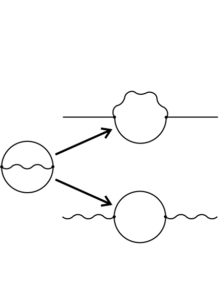
Figure 1: On the left the diagram representing the approximation for $V_{2}$ is depicted. Via functional variation one obtains the self-energy contributions to the pion and $\rho$-meson self-energies as on the ride hand side. The wiggled line represent the $\rho$-meson propagator and the solid line the pion propagator. The diagrams have to be resummed self-consistently.

This scheme does not include any resummation corrections of the vertices, so in $V_{2}$ one takes the vertices of the $\pi-\rho$ interaction stemming from the Lagrangian density (7) on the tree-level.

Calculating the self-energies for example for the $\rho$-mesons according to eqn. (11) corresponds on the diagrammatic level to cutting the $\rho$-propagator in the diagram of $V_{2}$. In an analogous way one obtains the self-energy of the pion (see fig. 1) . The scheme is self-consistent. Because every propagator appearing in the self-energy contributions is a full-propagator, i.e. in a perturbative language the propagators in the loop diagrams are fully resummed on that loop level.

The self-energies of the pions and the $\rho^{0}$-meson are therefore given by (11):

$$\Pi(P)=2\frac{\delta V_{2}}{\delta{\cal P}(P)}=-4g^{2}\int_{Q}(2P-Q)^{\mu}(2P-Q)^{\nu}{\cal S}_{\mu\nu}(Q){\cal P}(P-Q)$$

and

$$\Pi_{\mu\nu}(P)=2\frac{\delta V_{2}}{\delta{\cal S}^{\mu\nu}(P)}=-2g^{2}\int_{Q}(2Q-P)_{\mu}(2Q-P)_{\nu}{\cal P}(Q){\cal P}(P-Q)\,\,.$$ (14)

It is obvious that these self-energies themselves functionally depend on the propagators which enter the Dyson-Schwinger equations.

As we are interested in the dilepton emission from a medium in thermal equilibrium, we need to calculate the retarded propagator of the $\rho$-meson in thermal field theory, see e.g. LeBellac (2000). That quantity directly enters the calculation of the dilepton production rates. For that purpose we recall that the thermal average $\langle\hat{A}\rangle$ of an operator $\hat{A}$ is defined by

$$\langle\hat{A}\rangle_{\beta}=\frac{1}{Z(\beta)}{\rm Tr}\big{(}\hat{A}{\rm e}^{-\beta\hat{H}}\big{)}\,\,,$$ (15)

where $\hat{H}$ is the Hamiltonian, $\beta=1/T$ is the inverse temperature and $Z(\beta)$ is the partition sum. The retarded propagators of the $\rho$-meson and the pions are defined as follows:

$${\cal S}^{\mu\nu}_{\rm R}(t) = -i\langle\theta(t)[\hat{A}^{\mu}(t),\hat{A}^{\nu}(0)]\rangle_{\beta}\,\,,$$

$${\cal P}_{\rm R}(t) = -i\langle\theta(t)[\hat{\phi}(t),\hat{\phi}(0)]\rangle_{\beta}\,\,.$$ (16)

They can be expressed in terms of the spectral functions of the $\rho$-meson and the pions:

$${\cal S}^{\mu\nu}_{\rm R}(k_{0},{\bf k}) = \int_{-\infty}^{\infty}\frac{dp_{0}^{\prime}}{2\pi}\frac{\rho^{\mu\nu}(p_{0}^{\prime},{\bf k})}{k_{0}-p_{0}^{\prime}+i\eta^{\prime}}\,\,,$$

$${\cal P}_{\rm R}(k_{0},{\bf k}) = \int_{-\infty}^{\infty}\frac{dp_{0}^{\prime}}{2\pi}\frac{\rho(p_{0}^{\prime},{\bf k})}{k_{0}-p_{0}^{\prime}+i\eta^{\prime}}\,\,,$$ (17)

where an analytical continuation from Matsubara frequencies to real energies has been performed.

The vector meson propagator is a Lorentz-tensor. Lorentz invariance is broken because the 4-vector of the medium defines a preferred frame of reference and the tensorial densities (as spectral functions, self-energies, propagators) become functions of energy and of momentum. To identify the physically propagating modes of the vector meson, we project its propagators, self-energies and spectral function onto the four-dimensionally transverse and longitudinal subspaces. A detailed overview of the conventions of the projection formalism is given in appendix A .

Every tensorial quantity can be decomposed into the four-dimensionally transverse components (proportional to the projectors A and B) and longitudinal components (proportional to the projectors C, E), see eqn. (44).

In general the spectral function components can be expressed via:

$$\rho_{\rm A}(k_{0},{\bf k}) = -2{\rm Im}\,\frac{1}{2}{\rm A}_{\mu\nu}(k_{0},{\bf k})D^{{\rm R}\mu\nu}(k_{0},{\bf k})=-\,{\rm Im}\int_{-\infty}^{\infty}\frac{dk_{0}^{\prime}}{2\pi}\frac{{\rm A}_{\mu\nu}(k_{0},{\bf k})\rho^{\mu\nu}(k_{0}^{\prime},{\bf k})}{k_{0}-k_{0}^{\prime}+i\eta}$$

$$= \frac{1}{2}{\rm A}_{\mu\nu}\rho^{\mu\nu}\,\,,$$

$$\rho_{\rm B}(k_{0},{\bf k}) = -2{\rm Im}\,{\rm B}_{\mu\nu}(k_{0},{\bf k})D^{{\rm R}\mu\nu}(k_{0},{\bf k})=-2{\rm Im}\int_{-\infty}^{\infty}\frac{dk_{0}^{\prime}}{2\pi}\frac{{\rm B}_{\mu\nu}(k_{0},{\bf k})\rho^{\mu\nu}(k_{0}^{\prime},{\bf k})}{k_{0}-k_{0}^{\prime}+i\eta}$$

$$= {\rm B}_{\mu\nu}(k_{0},{\bf k})\rho^{\mu\nu}(k_{0},{\bf k})\,\,,$$

$$\rho_{C}(k_{0},{\bf k}) = -2\,{\rm Im}\,\left(-\frac{1}{2k_{0}^{2}k^{2}}{\rm C}_{\mu\nu}(k_{0},{\bf k})D^{{\rm R}\mu\nu}(k_{0},{\bf k})\right)$$

$$= \frac{1}{k_{0}^{2}k^{2}}\,{\rm Im}\int_{-\infty}^{\infty}\frac{dk_{0}^{\prime}}{2\pi}\frac{{\rm C}_{\mu\nu}(k_{0},{\bf k})\rho^{\mu\nu}(k_{0}^{\prime},{\bf k})}{k_{0}-k_{0}^{\prime}+i\eta}$$

$$= -\frac{1}{2k_{0}^{2}k^{2}}{\rm C}_{\mu\nu}(k_{0},{\bf k})\rho^{\mu\nu}(k_{0},{\bf k})\,\,,$$

$$\rho_{E}(k_{0},{\bf k}) = -2\,{\rm Im}\,{\rm E}_{\mu\nu}(k_{0},{\bf k})D^{{\rm R}\mu\nu}(k_{0},{\bf k})=-2\,{\rm Im}\int_{-\infty}^{\infty}\frac{dk_{0}^{\prime}}{2\pi}\frac{{\rm E}_{\mu\nu}(k_{0},{\bf k})\rho^{\mu\nu}(k_{0}^{\prime},{\bf k})}{k_{0}-k_{0}^{\prime}+i\eta}$$ (18)

$$= {\rm E}_{\mu\nu}(k_{0},{\bf k})\rho^{\mu\nu}(k_{0},{\bf k})\,\,.$$

The retarded propagator can be rewritten in terms of these spectral function’s components:

$${\cal S}_{{\rm R}\mu\nu}(k_{0},{\bf k})=\int_{-\infty}^{\infty}\frac{dk_{0}^{\prime}}{2\pi}\frac{\left(\rho_{\rm A}{\rm A}_{\mu\nu}+\rho_{\rm B}{\rm B}_{\mu\nu}+\rho_{\rm C}{\rm C}_{\mu\nu}+\rho_{\rm E}{\rm E}_{\mu\nu})(k_{0}^{\prime},{\bf k}\right)}{k_{0}-k_{0}^{\prime}+i\eta}.$$ (19)

Inverting the resummed propagator (see eqn. 9a) of the $\rho$-meson and employing eqns. (III) leads to:

$$\rho_{\rm A} = -2{\rm Im}\,\frac{1}{2}{\rm A}_{\mu\nu}(p_{0},{\bf p}){\cal S}^{\mu\nu}(p_{0},{\bf p})=-2\,{\rm Im}\,\left[\frac{1}{P^{2}-m^{2}+\Pi_{a}}\right]\,\,,$$

$$\rho_{\rm B} = -2{\rm Im}\,{\rm B}_{\mu\nu}(p_{0},{\bf p}){\cal S}^{\mu\nu}(p_{0},{\bf p})=-2{\rm Im}\,\left[b^{-1}(P)\right]\,\,,$$

$$\rho_{\rm C} = -2\,{\rm Im}\,\frac{1}{-2p_{0}^{2}p^{2}}{\rm C}_{\mu\nu}(p_{0},{\bf p}){\cal S}^{\mu\nu}(p_{0},{\bf p})\,\,$$

$$= -2\xi{\rm Im}\,\left[-b(P)\frac{P^{2}-\xi m^{2}+\xi\Pi_{e}}{\Pi_{c}}\right]^{-1}\,\,,$$

$$\rho_{\rm E} = -2\,{\rm Im}\,{\rm E}_{\mu\nu}(p_{0},{\bf p}){\cal S}^{\mu\nu}(p_{0},{\bf p})$$ (20)

$$= -2\xi{\rm Im}\,\left[b(P)\frac{P^{2}-\xi m^{2}+\xi\Pi_{e}}{P^{2}-m^{2}+\Pi_{b}}\right]^{-1}\,\,,$$

where the function $b(P)$ is given by

$$b(P)=P^{2}-m^{2}+\Pi_{b}+\xi\frac{p_{0}^{2}p^{2}\Pi_{c}^{2}}{P^{2}-\xi m^{2}+\xi\Pi_{e}}\,\,$$ (21)

and the projected components $\Pi_{a}$, $\Pi_{b}$, $\Pi_{c}$, and $\Pi_{e}$ (see appendix A) of the self-energy $\Pi_{\mu\nu}$ are introduced. The quantity $\xi$ is the gauge parameter appearing in the Stückelberg method in the $R_{\xi}$-gauge (see eqn. (3)).

In spite of the truncation of the resummation (e.g. limiting the sum of the two-particle irreducible diagrams $V_{2}$ to a subset of all possible digagrams) conservation of conserved currents stemming from global symmetries as long as they are realised as linear representations of the conserved group detailed balance and unitarity as well as thermodynamical consistence. This is guaranteed in $\Phi$-functional approximation schemes, as shown by Baym Baym (1962). However, in these schemes the vertex corrections necessary to guarantee Ward Takahashi identies for the propagator are not taken into account consistently. This shortcoming can lead to serious problems of the self-consistent treatment of vector particles on the propagator level van Hees (2000).

This problem has to be addressed in our scheme as well. In van Hees (2003) it has been shown that in order to be consistent with the corresponding Ward Takahashi identities the following relation: :

$$P^{\mu}{\cal S}^{\rm Stueck}_{\mu\nu} = \xi\frac{P_{\nu}}{P^{2}+\xi m^{2}}\,\,$$ (22)

for the (fully resummed) propagator of the massive vector meson $\cal{S}_{\mu\nu}$ has to be fulfilled in the Stückelberg theory. From that condition one can conclude that in Stückelberg theories (as in QED) the self-energy tensor of the vector particle has to be four-dimensionally transverse which corresponds to vanishing $\Pi_{c}$ and $\Pi_{e}$ components of the self-energy tensor.

This relation on the correlator level is spoiled in the employed $\Phi$-functional approximation, since only a partial resummation is performed. This fact is well known, not only for Stückelberg theories van Hees and Knoll (2000), but also from Dyson-Schwinger approaches to the description of QCD phenomena von Smekal et al. (1998) and stems from a violation of the gauge symmetry.

One may think that these fundamental considerations of the violation of Ward Takahashi identies don’t matter from a phenomenological point of view, because we are interested only in an apropriate description of the $\rho$-meson studying it’s importance for the understanding of dilepton spectra and not about intrinsically complicated considerations on the violation of local symmetries in gauge theories. But we calculate the production of dileptons in a VMD approach where the $\rho$-meson couples directly to the virtual photon, these questions have to be addressed in detail. In part B of the appendix the equation for the rate of dilepton production is given. Eqn. (53) shows that the current-current correlator is directly proportional to the retarded propagator of the $\rho$-meson. Current conservation in QED which is essential for an appropriate description of the dilepton production tells that the spectral-function of the $\rho$-meson has to be four-dimensionally transverse: $P_{\mu}\rho^{\mu\nu}=0$.

To guarantee conservation of the hadronic electromagnetic current, we work in an appropriate gauge: the $R_{\xi}$-gauge taking $\xi\rightarrow 0$ . This leads to the following modification of the eqns.:

$$\rho_{\rm A} = -2{\rm Im}\,\frac{1}{2}{\rm A}_{\mu\nu}(p_{0},{\bf p}){\cal S}^{\mu\nu}(p_{0},{\bf p})=-2\,{\rm Im}\,\left(P^{2}-m^{2}+\Pi_{a}\right)^{-1}\,\,,$$

$$\rho_{\rm B} = -2{\rm Im}\,{\rm B}_{\mu\nu}(p_{0},{\bf p}){\cal S}^{\mu\nu}(p_{0},{\bf p})=-2\,{\rm Im}\,\left(P^{2}-m^{2}+\Pi_{b}\right)^{-1}\,\,,$$

$$\rho_{\rm C} = -2\,{\rm Im}\,\frac{1}{-2p_{0}^{2}p^{2}}{\rm C}_{\mu\nu}(p_{0},{\bf p}){\cal S}^{\mu\nu}(p_{0},{\bf p})=0\,\,,$$

$$\rho_{\rm E} = -2\,{\rm Im}\,{\rm E}_{\mu\nu}(p_{0},{\bf p}){\cal S}^{\mu\nu}(p_{0},{\bf p})=0\,\,.$$ (23)

The components $\rho_{C}$ and $\rho_{E}$ do vanish and the transversality of the spectral-function $P^{\mu}\rho_{\mu\nu}=0$ and therefore current conservation is guaranteed. In that way we solve the most serious problem, mainly former violation of electromagnetic current conservation. On the level of the $\rho$-meson self-energy we still have non-vanishing $\Pi_{c}$ and $\Pi_{e}$ components, but this does not lead to problems calculating the dilepton rates. In the following we refer to this technique to guarantee the transversality of the spectral functions as ”approach I”.

In van Hees and Knoll (2000) the authors use a different ansatz by forcing the self-energy of the $\rho$-meson to be explicitly transverse via the eqns. (47) (with $X\equiv\Pi$), which are violated in $\Phi$-functional approximation schemes. In this ansatz one argues that the temporal components of the self-energy tensor are tied to the conseration of charge and therefore involve an infinite relaxation time of the conserved quantity in the full theory. The self-consistent results are different because they reflect the damping time of the propagators in the loop. This behaviour has been studied in detail in Knoll and Voskresensky (1996), where it has been shown that current conservation could be restored via a Bethe-Salpeter ladder resummation. The spatial components of the self-energy tensor are in general be less affected by the resummation in the case that the relaxation time for the transverse current-current correlator is comparable to the damping time of the propagators appearing in the loop, whereas the time components are expected to suffer significant changes van Hees and Knoll (2000). This physical reasoning leads to enforcing the transversality of the self-energy tensor via the first two eqns. of (47) (with $X\equiv\Pi$), which give the $\rho$-mesons four-dimensionally transverse self-energy components ($\Pi_{a}$, $\Pi_{b}$) as functions of $\Pi^{t}(P)=\frac{1}{2}\,\left(\delta^{ij}-\hat{p}^{i}\,\hat{p}^{j}\right)\,\Pi^{ij}(P)$ and $\Pi^{\ell}(P)=\hat{p}_{i}\,\Pi^{ij}(P)\,\hat{p}_{j}$:

$$\Pi^{\rm a}(P) = -\Pi^{t}(P)\,\,,$$ (24a)

$$\Pi^{\rm b}(P) = -\frac{P^{2}}{p_{0}^{2}}\Pi^{\ell}(P)\,\,.$$ (24b)

These equations are equivalent to eqn. (4) in van Hees and Knoll (2000) up to a different sign convention. In the following we refer to this technique to guarantee the transversality of the self-energy tensor first employed in van Hees and Knoll (2000) as ”approach II”.

For the sake of simplicity we are concentrating on damping width effects of the particles and avoid renormalization which would require a temperature independent self-consistent subtraction of infinities van Hees and Knoll (2002a) and don’t take into account any changes in the real part of the self-energies. This ansatz to disregards any mass shift of the particles is analogous to the one in van Hees and Knoll (2000).

Given the fact that we are interested in the phenomenology of the broadening due to finite width of the pions this approximation of neglecting mass shifts (i. e. disregarding renormalization), can be justified. In Gale and Kapusta (1991) the $\pi$-$\rho$ interaction has been studied perturbatively. The value of the mass shifts (relative to vacuum) predicted from this perturbative study are comparable with the mass shifts one can expect in any many body scheme. (This is different regarding the collisional broadening, since in the perturbative calculation the width of the pion giving raise to the $\rho$ meson’s width is zero.) Especially from Fig. 6, 7, 8 and, Fig. 9 in Gale and Kapusta (1991) one expects physical mass shifts from the $\pi$-$\rho$-interaction only in the range of about $10\%$ of the vacuum mass of the $\rho$-meson even for comparably high temperatures.

In that way, the equations for the non-vanishing components of the spectral function are:

$$\rho_{\rm A} = \frac{-2\,{\rm Im}\,\Pi_{a}}{(P^{2}-m^{2})^{2}+({\rm Im}\,\Pi_{a})^{2}}\,\,,$$

$$\rho_{\rm B} = \frac{-2\,{\rm Im}\,\Pi_{b}}{(P^{2}-m^{2})^{2}+({\rm Im}\,\Pi_{b})^{2}}\,\,$$

$$\rho_{\rm C} = 0\,\,$$

$$\rho_{\rm E} = 0\,\,$$ (25)

To close this self-consistent set of equations, we have to express the self-energies as functionals of the spectral function of the pion and the spectral function’s components $\rho_{a}$ and $\rho_{b}$ of the $\rho$-meson. We use the decomposition of the spectral function of the $\rho$-meson:

$$\rho_{\mu\nu}(P) = A_{\mu\nu}\rho_{a}(P)+B_{\mu\nu}\rho_{b}(P)=$$

$$= \bigg{(}-\delta_{ij}+\hat{p}_{i}\hat{p}_{j}\bigg{)}\rho_{a}(P)+\bigg{(}g_{\mu\nu}+\delta_{ij}-\frac{P_{\mu}P_{\nu}}{P^{2}}-\hat{p}_{i}\hat{p}_{j}\bigg{)}\rho_{\rm b}(P)\,\,,$$

where $\hat{p}_{i}$ is the normalized i.th component of the momentum vector $\hat{p}_{i}=p_{i}/p$ and the following contractions

$$g_{\mu\nu}(2P-Q)^{\mu}(2P-Q)^{\nu} = 2(P^{2}+L_{2}^{2})-L_{1}^{2}\,\,,$$

$$\frac{Q_{\mu}Q_{\nu}}{Q^{2}}(2P-Q)^{\mu}(2P-Q)^{\nu} = \frac{(P^{2}-L_{2}^{2})^{2}}{L_{1}^{2}}\,\,,$$

$$\delta_{ij}(2p-q)^{i}(2p-q)^{j} = 2(p^{2}+l_{2}^{2})-l_{1}^{2}\,\,,$$

$$\frac{q_{i}q_{j}}{q^{2}}(2p-q)^{i}(2p-q)^{j} = \frac{(p^{2}-l_{2}^{2})^{2}}{l_{1}^{2}}\,\,.$$ (26)

where $L_{1}=Q$ and $L_{2}=P-Q$. The quantities $l_{1}^{2},l_{2}^{2}$, and $p^{2}$ are the squared three-momenta. $l_{10}$ and $l_{20}$ are the energy components of $L_{1}$ and $L_{2}$, respectively. We obtain the following equation of part of the self-energy of the pion:

$${\rm Im}\Pi(P)= -\pi\frac{4g^{2}}{p(2\pi)^{2}}\int_{0}^{\infty}l_{1}{\rm d}l_{1}\int_{0}^{\infty}l_{2}{\rm d}l_{2}\int_{-\infty}^{\infty}\frac{{\rm d}l_{10}}{2\pi}\int_{-\infty}^{\infty}\frac{{\rm d}l_{20}}{2\pi}$$ (27)

$$\times\bigg{\{}-\left[2(p^{2}+l_{2}^{2})-l_{1}^{2}-\frac{(p^{2}-l_{2}^{2})^{2}}{l_{1}^{2}}\right]\rho_{a}(l_{10},l_{1})$$

$$~{}-\big{[}2(P^{2}+L_{2}^{2})-L_{1}^{2}+2(p^{2}+l_{2}^{2})-l_{1}^{2}-\frac{(P^{2}-L_{2}^{2})^{2}}{L_{1}^{2}}$$

$$~{}-\frac{(p^{2}-l_{2}^{2})^{2}}{l_{1}^{2}}\big{]}\rho_{b}(l_{10},l_{1})\bigg{\}}\rho(l_{20},l_{2})$$

$$~{}\times\Theta\left(|l_{1}-l_{2}|\leq p\leq l_{1}+l_{2}\right)$$

$$~{}\times\left[1+f(l_{10})+f(l_{20})\right]\delta(p_{0}-l_{10}-l_{20})\,\,.$$

To determine the imaginary four-dimensionally transverse components of the self-energy ${\rm Im}\,\Pi_{a}$ and ${\rm Im}\,\Pi_{b}$, we employ eqns. (46)(with $X\equiv\Pi$) and use the following contactions:

$$\delta_{ij}(2q-p)^{i}(2q-p)^{j} = 2(l_{1}^{2}+l_{2}^{2})-p^{2}\,\,,$$

$$\frac{p_{i}p_{j}}{p^{2}}(2q-p)^{i}(2q-p)^{j} = \frac{(l_{1}^{2}-l_{2}^{2})^{2}}{p^{2}}\,\,,$$

$$(2q-p)^{0}(2q-p)^{0} = (l_{10}-l_{20})^{2}\,\,,$$

$$(2q-p)^{0}(2q-p)_{i}\frac{p^{i}}{p} = -\frac{(l_{10}-l_{20})(l_{1}^{2}-l_{2}^{2})}{p}\,\,,$$ (28)

We need to calculate ${\rm Im}\left(\delta^{ij}\Pi_{ij}\right)$, ${\rm Im}\left(\hat{p}^{i}\hat{p}^{j}\Pi^{ij}\right)$, ${\rm Im}\left(\Pi^{00}\right)$ and ${\rm Im}\left(\Pi^{i0}\hat{p}_{i}\right)$. These are given by:

$${\rm Im}\,\left(\delta^{ij}\Pi_{ij}\right) = -\pi\frac{2g^{2}}{p(2\pi)^{2}}\int_{0}^{\infty}l_{1}{\rm d}l_{1}\int_{0}^{\infty}l_{2}{\rm d}l_{2}\int_{-\infty}^{\infty}\frac{{\rm d}l_{10}}{2\pi}\int_{-\infty}^{\infty}\frac{{\rm d}l_{20}}{2\pi}$$ (29a)

$$~{}\times\left[2(l_{1}^{2}+l_{2}^{2})-p^{2}\right]\rho(l_{10},l_{1})\rho(l_{20},l_{2})\delta\left(p_{0}-l_{10}-l_{20}\right)$$

$$~{}\times~{}\Theta\left(|l_{1}-l_{2}|\leq p\leq l_{1}+l_{2}\right)$$

$$~{}\times~{}\left[1+f(l_{10})+f(l_{20})\right],$$

$${\rm Im}\,\left(\hat{p}_{i}\hat{p}_{j}\Pi^{ij}\right) = -\pi\frac{2g^{2}}{p(2\pi)^{2}}\int_{0}^{\infty}l_{1}{\rm d}l_{1}\int_{0}^{\infty}l_{2}{\rm d}l_{2}\int_{-\infty}^{\infty}\frac{{\rm d}l_{10}}{2\pi}\int_{-\infty}^{\infty}\frac{{\rm d}l_{20}}{2\pi}$$ (29b)

$$~{}\times\left[\frac{(l_{1}^{2}-l_{2}^{2})^{2}}{p^{2}}\right]\rho(l_{10},l_{1})\rho(l_{20},l_{2})\delta\left(p_{0}-l_{10}-l_{20}\right)$$

$$~{}\times~{}\Theta\left(|l_{1}-l_{2}|\leq p\leq l_{1}+l_{2}\right)$$

$$~{}\times~{}\left[1+f(l_{10})+f(l_{20})\right],$$

$${\rm Im}\left(\Pi^{00}\right) = -\pi\frac{2g^{2}}{p(2\pi)^{2}}\int_{0}^{\infty}l_{1}{\rm d}l_{1}\int_{0}^{\infty}l_{2}{\rm d}l_{2}\int_{-\infty}^{\infty}\frac{{\rm d}l_{10}}{2\pi}\int_{-\infty}^{\infty}\frac{{\rm d}l_{20}}{2\pi}$$ (29c)

$$~{}\times\left[(l_{10}-l_{20})^{2}\right]\rho(l_{10},l_{1})\rho(l_{20},l_{2})\delta\left(p_{0}-l_{10}-l_{20}\right)$$

$$~{}\times~{}\Theta\left[|l_{1}-l_{2}|\leq p\leq l_{1}+l_{2}\right]$$

$$~{}\times~{}\left[1+f(l_{10})+f(l_{20})\right]\,\,,$$

and

$${\rm Im}\left(\Pi^{i0}\hat{p}_{i}\right) = -\pi\frac{2g^{2}}{p(2\pi)^{2}}\int_{0}^{\infty}l_{1}{\rm d}l_{1}\int_{0}^{\infty}l_{2}{\rm d}l_{2}\int_{-\infty}^{\infty}\frac{{\rm d}l_{10}}{2\pi}\int_{-\infty}^{\infty}\frac{{\rm d}l_{20}}{2\pi}$$ (29d)

$$~{}\times\left[-\frac{(l_{10}-l_{20})(l_{1}^{2}-l_{2}^{2})}{p})\right]\rho(l_{10},l_{1})\rho(l_{20},l_{2})$$

$$~{}\times~{}\Theta\left(|l_{1}-l_{2}|\leq p\leq l_{1}+l_{2}\right)\delta\left(p_{0}-l_{10}-l_{20}\right)$$

$$~{}\times~{}\left[1+f(l_{10})+f(l_{20})\right]\,\,.$$

With this set of equations for the self-energy and spectral-density components, we have established our self-consistently resummed approximation scheme. We solve this set of equations numerically.

IV Finite width-effects on the $\rho$-meson

In order to gain insight into the physics employing the spectral modifications, we compare the result with the resummational approach of the previous section to perturbative one-loop calculations of the $\rho$- (cf. Geddes (1980)) and $\pi$ widths.

As outlined in the last section, we work in the $\Phi$-functional approximation scheme in the $R_{\xi}$-gauge with $\xi\rightarrow 0$, which is a choice guaranteeing decoupling of the Stückelberg and Fadeev Popov ghost from the $\rho$ vector meson field and fulfilling the transversality condition of the electromagnetic current (therefore respecting QED gauge invariance). Nonetheless as mentioned before this cannot cure the violation of the Ward Takahashi identities stemming from the violation of local gauge invariance by the $\Phi$-functional approach. That is why we also compare our method to the results obtained by the enforcement of the transversality condition by disregarding the temporal contributions of the tensor (which is spoiling somewhat the $\Phi$-functional approach) which has been suggested and studied by van Hees and Knoll (2000) in a similar model. We concentrate on the $\rho$-$\pi$ interaction.

In order to gain information to what extend this influences the effects which we are interested in, we discuss the broadening effects in the full $\Phi$-functional approach (referred to as approach I) and in the transversality-enforcing resummation scheme (referred to as approach II).

The phenomenological most important difference between the resummation approaches and the perturbative one is, that the perturbatively calculated self-energies of the $\rho$-meson show a threshold behavior: the self-energies for timelike momenta vanish if $\sqrt{P^{2}}<2m_{\pi}$, where $P$ is the four-momentum of the meson relative to the rest frame of the medium. This leads to a characteristic threshold in the dilepton-spectra: only lepton-pairs with invariant masses above $2m_{\pi}$ are emitted. Considering the self-energy components of the $\rho$-meson in the self-consistent resummation scheme employed here shows that the finite width of the pions smears out this perturbative threshold behavior: the whole spectrum of invariant masses of the dileptons becomes accessible. Therefore this threshold ought to be considered as an artefact of the perturbative calculation.

IV.1 Self-energies and spectral densities

We start our discussion with the four-dimensionally transverse self-energy components ${\rm Im}\Pi_{a}$ and ${\rm Im}\Pi_{b}$ of the $\rho$-meson. The ${\rm Im}\Pi_{a}$-component is spatial-transverse and the ${\rm Im}\Pi_{b}$-component is spatial-longitudinal. These components are plotted as a function of energy for a fixed momentum $p=125{\rm MeV/c}$ relative to the medium for three different temperature in fig. 2(left and middle).

Figure 2: The imaginary parts of the spatial-transverse and spatial- longitudinal self-energies $\Pi_{a}$ and $\Pi_{b}$, respectively, as a function of energy at a constant momentum of $p=125~{}{\rm MeV}/c$ on the left hand side and in the middle. We show the results for a perturbative calculation and for the self-consistent calculations using the full $\Phi$-functional approach (approach I) and the transversality-enforcing approach (approach II). The imaginary part of the negative of the pion’s self-energy is depicted on the right hand side. The perturbative self-energy of the pion is too small to be seen on the scale of the graph on the right hand side.

In both self-consistent approaches the spatial transverse and spatial longitudinal imaginary parts of the self-energies show that there is no two-pion threshold. The perturbatively calculated imaginary parts of the self-energies can be compared to the self-consistent ones and vanish for $0<\sqrt{P^{2}}=\sqrt{p_{0}^{2}-p^{2}}<2m_{\pi}$.

The self-energy projectors are (up to possible poles and cuts) analytic functions in the complex energy-plane. Possible cuts on the real energy-axes corresponding to the imaginary part of the self-energy projections separate the upper and lower half-planes LeBellac (2000). Because of the anti-symmetry of the imaginary-parts of the self-energy projectors these cuts extend in the self-consistent calculations (approach I and approach II) over the total axes. The retarded functions in the upper half plane are therefore totally separated from the advanced in the lower plane. This leads in both self-consistent approaches to a (static) dilepton-rate that has no two-pion-threshold behavior as discussed below.

In approach I the ${\rm Im\Pi}_{b}$-component shows another remarkable property. It has not only a change of sign at the light-cone (that means at the transition between time- and spacelike momenta for $p_{0}=p$), but also a singularity. The transversality-condition $P^{\mu}\Pi_{\mu\nu}$ means on that level that for $P^{2}=0$ the component ${\rm Im}\Pi_{b}$ has to vanish. Indeed, that is not fulfilled in the $\Phi$-derivable approach (approach I), but is enforced in approach II. In approach II the self-energy component ${\rm Im}\Pi_{b}$ remains a continous function of $p_{0}$ even in the vincinity of the light-cone.

Eqn.(46b) shows that the energy component can have a $1/P^{2}$-pole that leads to a change of sign in ${\rm Im}\Pi_{b}$ at $p_{0}=p$ as obsvered in approach I. This is an artefact of approach I that is closely correlated to the violation of the transversality condition of the self-energy tensor $\Pi_{\mu\nu}$, see also the discussion in section III. Although transversality of the self-energy components is violated, the spectral-density tensor $\rho_{\mu\nu}$ still remains four-transverse in the $R_{\xi}$-gauge for $\xi\rightarrow 0$ guaranteeing the conservation of the hadronic-electromagnetic current. Therefore approach I is consistent within the vector meson dominance approach with quantum electrodynamics, as already discussed above. The singularity of strength $1/P^{2}$ of the ${\rm Im\Pi}_{b}$-component at the light-cone still leads to a continuous behavior of $\rho_{b}$ at $p_{0}=p$.

In figure 3 we plot the components of the spectral-function of the $\rho$-meson at a temperature $T=100\,{\rm MeV}$ as a function of energy $p_{0}$ and momentum $p$ as obtained within the self-consistent approach I.

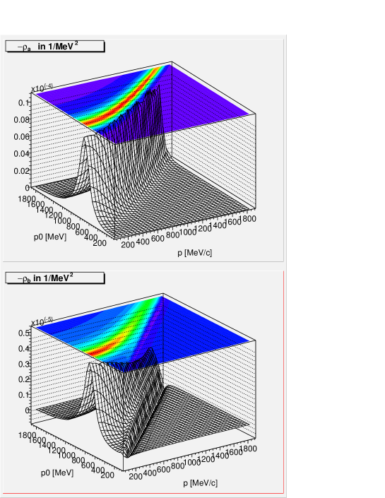
Figure 3: (Color online) The spatial-transverse and spatial- longitudinal spectral functions $\rho_{a}$ and $\rho_{b}$, respectively, of the rho meson as a function of energy and momentum on at a temperature of 100 MeV in the full $\Phi$-functional approach (approach I).

We plot the corresponding spatial-transverse and spatial-longitudinal components of the spectral function of the $\rho$-meson depending on $\sqrt{P^{2}}=\sqrt{p_{0}^{2}-p^{2}}$ for a given momentum of $p=125~{}{\rm MeV/c}$ for three different temperatures, the two self-consistent approaches and the perturbative calculation in figure 4.

Figure 4: The spatial-transverse and spatial- longitudinal spectral functions $\rho_{a}$ and $\rho_{b}$, respectively, of the rho meson are given as a function of invariant mass at a constant momentum of $p=125MeV/c$ on the left hand side. We give the results for the perturbative calculation and for the self-consistent appoaches I and II (see text). The perturbative spatial-transverse and spatial-longitudinal components are within the resolution of the figure identical, that is why we used only one curve for both of them.

The spatial longitudinal and transverse components differ in both self-consistent calculations from each other only in the region about $0<\sqrt{P^{2}}<500\,{\rm MeV}$ and are for about $\sqrt{P^{2}}>500\,{\rm MeV}$ identical. With rising temperature this difference in the lower mass region is enhanced and the spectral components get in both self-consistent calculations considerably broadened. The perturbatively calculated spatial transverse and longitudinal spectral components (which are within the resultion of the figure almost identical) are considerably narrower and show no spectral strength below the two-pion-threshold. In figure 5 we show the components of the spectral-function of the pion at a temperature of $T=100{\rm MeV}$ as a function of energy $p_{0}$ and momentum $p$ for the self-consistent calculation within approach I.

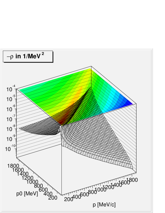
Figure 5: (Color online)The spectral function of the pion as as a function of energy and momentum at a temperature of 100 MeV as obtained within the self-consistent calculation applying approach I (see text).

Fig. 6 shows the $\pi$ spectral function for different T and a constant momentum of $p=125~{}{\rm MeV/c}$. It shows considerable broadening of the pion in both self-consistent approaches.

Figure 6: The spectral functions $\rho$ of the pion is given as a function of invariant mass at a constant momentum of $p=125MeV/c$ on the left hand side. We give the results for the perturbative calculation and for the self-consistent one. The width of the pion right hand side for the self-consistent and the perturbative calulation as a function of invariant mass.

Comparing to the perturbative calculation one oberserves apart from broadening the vanishing of the spectral function in the range between roughly $630$ and $910$ ${\rm MeV}$. This is due to the fact that for two particles with mass $m_{1}>m_{2}$ the perturbative calculation leads to a vanishing width for $m_{1}-m_{2}<\sqrt{P^{2}}<m_{1}+m_{2}$ - which corresponds to the two-pion threshold in the case of the $\rho$-meson and to the threshold behavior as mentioned here for the pions. This threshold behavior is no longer present in both self-consistent approaches.

IV.2 Static thermal dilepton rate

We proceed by calculating the static thermal dilepton emission rate in the model. For this purpose, we use eqn.(54), where this quantity for the hadronic channel is given as a function of the invariant dilepton mass and as a functional of the $\rho$-meson spectral function based on VMD (see appendix B for details). We calculate the rate for different T (see figure 7) for

Figure 7: The figure shows the static rate of dilepton (dielectron) production as a function of invariant mass. The decaying rho meson has a constant momentum of $p=125MeV/c$. We give the self-consistent results as obtained within approach I and approach II (see text for explanation) and the perturbative ones.

decaying $\rho$-mesons of momentum $p=125{\rm MeV/c}$ relative to the medium.

The dilepton emission rate increases with temperature. This enhancement is due to the Bose Einstein factor in eq. (54). The self-consistently calculated rates in approach I and II give rise to a larger yield in the low-mass part $M=\sqrt{P^{2}}<800\,{\rm MeV}$ of the spectrum than the perturbatively calculated rate which moreover has the two-pion threshold below $2m_{\pi}$. In the present model, this leads to a considerable enhancement of the dilepton-rate especially in the $\sqrt{P^{2}}<700\,{\rm MeV}$ sector in comparison to the perturbative predictions. The self-consistently calculated rates of approach I exhibit even larger broadening effects for the $\rho$-meson than those of approach II. Despite this difference both self-consistent approaches show clearly that in this part of the low mass dilepton region the collisional broadening effects enhance the expected static rates considerably and outweigh the two-pion threshold of the perturbative approach. Above $850\,{\rm MeV}$ there are no important difference in comparison with the perturbative results.

V Dilepton emission and fireball evolution

In order to demonstrate that the results of the previous section, especially the considerable collisional broadening of the $\rho$-meson leads to significant quantitative changes in the prediction of dilepton rates we model the fireball evolution and fold it with the rate calculations.

We emphasize that we study a simplified model of the medium considering only the self-consistent finite width effects of the $\rho$-$\pi$ interaction at finite T where other effects (like mass shifts, chiral symmetry, and scattering off by baryons) have not been included. We do not suggest that these effects are unimportant but wish to demonstrate the self-consistent description of collisional broadening already implies siginificant modifications.

V.1 The Fireball model

In order to obtain the complete emitted spectrum we use a mode for the fireball which has been shown to reproduce a number of other important observables Renk (2004a). Here, we briefly outline the framework.

The fundamental model assumption is that the fireball matter is in local thermal (but not necessarily in chemical) equilibrium from an initial proper-time scale $\tau_{0}$ till a later breakup at time $\tau_{f}$. We chose volumes corresponding to a given proper time $\tau$ for the calculation of thermodynamics. Assuming spatial homogeneity, temperature $T$, entropy density $s$, pressure $p$ and chemical potentials $\mu_{i}$ as well as energy-density $\epsilon$ become functions of $\tau$ in such a system.

The volume is assumed to be cylindrically symmetric around the z-axis of the beam. It is characterized by the longitudinal extension $L(\tau)$ and the transverse radius $R(\tau)$:

$$V(\tau)=\pi L(\tau)R^{2}(\tau).$$ (30)

In order to account for collective flow effects, we boost individual volume elements according to a position-dependent velocity field. For the transverse flow, we make the ansatz

$$\eta_{T}(r,\tau)=r/R_{rms}(\tau)\eta_{T}^{rms}(\tau)$$ (31)

where $R_{rms}(\tau)$ denotes the root mean square radius of the fireball at $\tau$ and $\eta_{T}^{rms}(\tau)$ the transverse rapidity at $R_{rms}$.

For the longitudinal dynamics, we start with the experimentally measured width of the rapidity interval of observed hadrons $2\eta_{f}^{front}$ at breakup. From this, we compute the longitudinal velocity of the fireball front at kinetic freeze-out $v_{f}^{front}$. We do not require the initial expansion velocity $v_{0}^{front}$ to coincide with $v_{f}^{front}$ but instead allow for a longitudinally accelerated expansion. This implies that during the evolution $\eta=\eta_{s}$ is not valid (with $\eta_{s}$ the spacetime rapidity $\eta_{s}=1/2\ln((t+z)/(t-z))$.

The requirement that the acceleration should be a function of $\tau$ and that the system stays spatially homogeneous for all $\tau$ determines the velocity field uniquely if the motion of the front is specified. We solve the resulting system of equations numerically Renk (2004a). We find that for not too large rapidities $\eta<4$ and accelerations volume elements approximately fall on curves $const.=\sqrt{t^{2}-z^{2}}$ and that the flow pattern can be approximated by a linear relationship between rapidity $\eta$ and spacetime rapidity $\eta_{s}$ as $\eta(\eta_{s})=\zeta\eta_{s}$ where $\zeta=\eta^{front}/\eta_{s}^{front}$ and $\eta^{front}$ is the rapidity of the cylinder front. In this case, the longitudinal extension can be found calculating the invariant volume $V=\int d\sigma_{\mu}u^{\mu}$ as

$$L(\tau)\approx 2\tau\frac{\text{sinh }((\zeta-1)\eta_{s}^{front}(\tau))}{(\zeta-1)}$$ (32)

with $\eta_{s}^{front}(\tau)$ the spacetime rapidity of the cylinder front. This is an approximate generalization of the boost-invariant relation $L(\tau)=2\eta^{front}\tau$ which can be derived for non-accelerated motion.

V.1.1 Parameters of the expansion

In order to proceed, we have to specify the longitudinal acceleration $a_{z}(\tau)$ (which in turn is used to calculate $\eta_{s}^{front}(\tau)$ numerically), the initial front velocity $v_{0}^{front}$ and the expansion pattern of the radius $R(\tau)$ in proper time.

For the acceleration we make the ansatz

$$a_{z}=c_{z}\cdot\frac{p(\tau)}{\epsilon(\tau)}$$ (33)

which allows a soft point in the EoS where the ratio $p/\epsilon$ gets small to influence the acceleration pattern. $c_{z}$ and $v_{0}^{front}$ are model parameters governing the longitudinal expansion and fit to data. Hence the EoS translates into a temperature (and proper-time $\tau$) and determines the acceleration profile $a=const.p(T)/\epsilon(T)$.

Since typically longitudinal expansion is characterized by larger velocities than transverse expansion, i.e. $v_{z}^{front}\gg v_{T}^{front}$, we treat the radial expansion non-relativistically. We assume that the radius of the cylinder can be written as

$$R(\tau)=R_{0}+c_{T}\int_{\tau_{0}}^{\tau}d\tau^{\prime}\int_{\tau_{0}}^{\tau^{\prime}}d\tau^{\prime\prime}\frac{p(\tau^{\prime\prime})}{\epsilon(\tau^{\prime\prime})}$$ (34)

The initial radius $R_{0}$ is taken from overlap calculations. This leaves a parameter $c_{T}$ determining the strength of transverse acceleration which is also fit to data. The final parameter characterizing the expansion is its endpoint given by $\tau_{f}$, the breakup proper time of the system.

V.1.2 Evolution of temperature

We assume that entropy is conserved throughout the thermalized expansion phase. Therefore, we start by fixing the entropy per baryon from the number of produced particles per unit rapidity (see e.g. Letessier et al. (1995)). Calculating the number of participant baryons (see Renk et al. (2002)) we find the total entropy $S_{0}$. The entropy density at a given proper time is then determined by $s=S_{0}/V(\tau)$.

We describe the EoS in the partonic phase by a quasiparticle interpretation of lattice data which has been shown to reproduce lattice results both at vanishing baryochemical potential $\mu_{B}$ and finite $\mu_{B}$ Schneider and Weise (2001).

For the phase transition temperature, we choose $T_{C}=170$ MeV based on lattice QCD computations at finite temperature for case of two light and one heavy quark flavour Karsch et al. (2001). We also note that no large latent heat is observed in lattice calculations for the transition and model the actual thermodynamics as a crossover rather than a sharp phase transition. Nevertheless, in the calculation we assume quarks and gluons as degrees of freedom above $T_{C}$ and hadrons below to simplify computations. Since the time the system spends in the vicinity of the transition temperature is small compared with the total time for dilepton emission, any error we make by this assumption is bound to be small as soon as we consider the measured rates which represent an integral over the time evolution of the system folded with the emission rate.

Since a computation of thermodynamic properties of a strongly interacting hadron gas close to $T_{C}$ is a very difficult task, we follow a simplified approach instead: We calculate thermodynamic properties of a hadron gas at kinetic decoupling where interactions cease to be important. Here, we have reason to expect that an ideal gas will be a good description and obtain the EoS using an ideal resonance gas model. Using the framework of statistical hadronization Renk (2003a), we determine the overpopulation of pion phase space by pions from decays of heavy resonances created at $T_{C}$ and include this contribution (which gives rise to a pion-chemical potential of order $\mu_{\pi}\approx 120$ MeV into the calculation). We then choose a smooth interpolation between decopling temperature $T_{f}$ and transition temperature $T_{C}$ to the EoS obtained in the quasiparticle description. This is described in greater detail in Renk et al. (2002).

With the help of the EoS and $s(\tau)$, we are now in a position to compute the parameters $p(\tau),\epsilon(\tau),T(\tau)$ as well. Since the ratio $p(\tau)/\epsilon(\tau)$ appear in the expansion parametrization, we have to solve the model self-consistently.

V.1.3 Solving the fireball-evolution-model

In order to adjust the model parameters, we compare with data on transverse momentum spectra and HBT correlation measurements. This is discussed in greater detail in Renk (2004b, a).

By requiring $R(\tau_{f})=R_{f}$ and $v_{T}^{front}=v_{\perp f}$ we can determine the model parameters $c_{T}$ and $\tau_{f}$. $c_{z}$ is fixed by the requirement $\eta^{front}(\tau_{f})=\eta_{f}^{front}$. The remaining parameter $v_{0}^{front}$ now determines the volume (and hence temperature) at freeze-out and can be adjusted such that $T(\tau_{f})=T_{f}$.

The model for 5% central 158 AGeV Pb-Pb collisions at SPS is characterized by the following scales: Initial long. expansion velocity $v_{0}^{front}=0.54c$, thermalization time $\tau_{0}=1$ fm/c, initial temperature $T_{0}=300$ MeV, duration of the QGP phase $\tau_{QGP}=6.5$ fm/c, duration of the hadronic phase $\tau_{had}=8.5$ fm/c, total lifetime $\tau_{f}-\tau_{0}=15$ fm/c, r.m.s radius at freeze-out $R_{f}^{rms}=8.55$ fm, transverse expansion velocity $v_{\perp f}=0.57c$.

For the discussion of dileptons, we require the fireball evolution for other than 5% central collisions. In this case, we make use of simple scaling arguments based on the initial overlap geometry and the number of collision participants. For a detailed description, see Renk et al. (2002); Polleri et al. (2004).

In Renk et al. (2002), it has been shown that this scenario is able to describe the measured spectrum of low mass dileptons, and in Renk (2003a) it has been demonstrated that under the assumption of statistical hadronization at the phase transition temperature $T_{C}$, the measured multiplicities of hadron species can be reproduced. In Polleri et al. (2004), the model has been shown to describe charmonium suppression correctly. None of these quantities is, however, very sensitive to the detailed choice of the equilibration time $\tau_{0}$. Therefore, we have only considered the ‘canonical’ choice $\tau_{0}=$ 1 fm/c so far. The calculation of photon emission within the present framework provides the opportunity to test this assumption and to limit the choice of $\tau_{0}$. In Renk (2003b), this has been investigated in some detail. Within the present framework, the limits $0.5$ fm/c $<\tau_{0}<$ $3$ fm/c could be found. Variations within these limits, however, do not affect the spectrum of dileptons with invariant mass below 1 GeV significantly.

V.2 Dileptons from the QGP Phase

In order to take into account the contributions from the phase of a QGP, we employ a quasiparticle picture Schneider and Weise (2001). The model treats quarks and gluons as massive thermal quasiparticles. The QCD dynamics is incorporated in the thermal masses of these ’effective’ quarks and gluons. The masses in this model approach the hard thermal loop (HTL) results at high temperature. Around $T_{c}$ a power law fall-off is assumed for the thermal masses, based on the conjecture that the phase transition is either weakly first order or second order. The thermodynamic quantities of the QGP are calculated in terms of two functions $B(T)$ and $C(T)$ introduced in the model, see ref. Schneider et al. (2002); Renk et al. (2002) , which account for the thermal vacuum energy and a phenomenological description of deconfinement. As long as the thermodynamically active degrees of freedom are quarks and gluons in a quasiparticle gas, the virtual photon couples electromagnetically only to the thermally excited $q\bar{q}$-states populating the plasma phase and converts into a lepton pair, for details see section 4.1 of Renk et al. (2002). This mechanism can be compared to the coupling of the virtual photon to the vector-meson in VMD in the hadronic phase.

As the preferred reference frame of hot matter breaks Lorentz invariance, new partonic excitations such as longitudinal gluonic plasmons or helicity-flipped plasminos could be present. Their spectral strength remains exponentially suppressed for high temperatures and momenta which dominate macroscopic thermodynamic quantities (pressure, entropy and energy density) and their contribution is neglected in a quasiparticle description. However, for soft-dilepton production these plasmino modes lead to sharp, distinct structures in the static dilepton-emission spectra, so called van Hove singularities Braaten et al. (1990) . These peaks should be roughly located at twice the thermal quasiparticle quark mass $\approx 2m_{q}(T)$ and would be smeared out by the fireball evolution, since the thermal quark masses drop with temperature. Furthermore, since in the quasiparticle model Schneider and Weise (2001) $m_{q}(T)$ is of order $T$ (smeared out) van Hove singularities could only appear at low invariant masses and would be overwhelmed by the hadronic part of the dilepton production. Therefore the effects of neglecting gluonic and (helicity-flipped) plasmino modes are expected to be neglible.

V.3 Dilepton Emission

Comparison with the measured dilepton spectrum is enabled by folding the differential rate $dN/(d^{4}xd^{4}q)=dR/d^{4}q$ with the space-time history of the collision. We want to compare the model predictions with the CERES/NA45 data Agakishiev et al. (1995, 1998); Lenkeit et al. (1999) taken in Pb-Au collisions at 158 AGeV (corresponding to a c.m. energy of $\sqrt{s}\sim 17$ AGeV) and 40 AGeV ($\sqrt{s}\sim 8$ AGeV). The CERES experiment is a fixed-target experiment. In the lab frame, the CERES detector covers the limited rapidity interval $\eta=2.1-2.65$, i.e. $\Delta\eta=0.55$. We integrate the calculated rates over the transverse momentum $p_{T}$ and average over $\eta$, given that $d^{4}p=Mp_{T}\ dM\ d\eta\ dp_{T}\ d\theta.$ The formula for the space-time- and $p$-integrated dilepton rate in the framework outlined above hence becomes

$$\frac{d^{2}N}{dMd\eta}=\frac{2\pi M}{\Delta\eta}\int\limits_{\tau_{0}}^{\tau_{f}}d\tau\ \int d\eta^{\prime}\ V(\eta^{\prime},T(\tau))\int\limits_{0}^{\infty}dp_{T}\ p_{T}\ \frac{dN(T(\tau),M,\eta^{\prime},p_{T})}{d^{4}xd^{4}p}\ Acc(M,\eta^{\prime},p_{T}),$$ (35)

where $\tau_{f}$ is the freeze-out proper time of the collision. $V(\eta,T(\tau))$ describes the proper time evolution of volume elements moving at different rapidities and the function $Acc(M,\eta,p_{T})$ accounts for the experimental acceptance cuts specific to the detector. At the CERES experiment, each electron/positron track is required to have a transverse momentum $p_{T}>0.2$ GeV, to fall into the rapidity interval $2.1<\eta<2.65$ in the lab frame and to have a pair opening angle $\Theta_{ee}>35$ mrad. Finally, for comparison with the CERES data, the resulting rate is divided by $dN_{ch}/d\eta$, the rapidity density of charged particles.

V.4 Hadronic cocktail in the vacuum

After freeze-out there are still hadrons present which decay after a finite time in vacuum and thus contribute to the dilepton yield. Below approximately $400$ MeV Dalitz decays are the dominant decay mechanism in this regime. We use the experimental analysis of the CERES collaboration for SPS conditions.

Most notably, remaining $\omega$ and $\phi$ mesons contribute a characteristic sharp peak structure due to their vacuum decays. We calculate their contribution directly from the model.

The direct decay of a vector meson $V$ into lepton pairs is given via:

$$\frac{dN_{V}}{dMd\eta}=\frac{1}{\Delta\eta}\ \frac{\alpha^{2}}{12\pi^{4}}\ R_{V}(M,T=0)\int_{\tau_{f}}^{\infty}d\tau\ V_{f}\int d^{3}q\ \frac{M}{q^{0}}\ f_{B}(q^{0},T_{f})\exp\left(-\frac{\tau-\tau_{f}}{\gamma(q)\tau_{0}^{V}}\right).$$

The temperatur $T_{f}=T(\tau_{f})$ and the volume $V_{f}=V(\tau_{f})$ of the the system are to be considered at freeze-out time $\tau_{f}$. After this time all medium effects vanish and the vacuum spectral function of the (virtual) photon $R_{V}(M,T=0)$ determines the rate of dilepton production. The momentum distribution of the vector mesons is given by the Bose-Einstein contribution determined by the temperature at freeze-out. Due to the decay of the mesons and the absence of thermal recombination effects the number of vector mesons is decreasing exponentially as $\exp\left(-(\tau-\tau_{f})/(\gamma(q)\tau_{0}^{V})\right)$. Here, $\tau_{0}^{V}$ is the vacuum life time of the vector meson. The quantity $\gamma(q)$ accounts for time dilatation effects on particles with finite three-momentum:

$$\gamma(q)=\frac{1}{\sqrt{1-v^{2}}}=\frac{q^{0}}{M}.$$

Integrating over proper time one obtains:

$$\frac{dN}{dMd\eta}=\frac{1}{\Delta\eta}\frac{\alpha^{2}}{12\pi^{4}}\tau_{0}R(M,T=0)V_{f}\int d^{3}q\ f_{B}(q^{0},T_{f}).$$

The averaged four-dimentional space-time volume available after freeze-out is as one would expect: $V_{f}\tau_{0}^{V}$. The three-momentum integral yields the particle density of virtual photons as a function of the invariant mass: $n(M)=N(M)/V$. Multiplying the factor $V_{f}$ one obtains the total number of virtual photons decaying in the freeze-out stage.Weighting this with $R_{V}(M)$ this gives the $dN/dM$ distribution for the process in the freeze-out stage vector-meson $\rightarrow\gamma^{*}\rightarrow e^{+}e^{-}$.

VI Dilepton invariant mass spectra

Once the time evolution is given in terms of the temperature $T(\tau)$, baryon density $\rho(\tau)$ and the knowledge of the dilepton rates from the hadronic medium at finite temperature and at freeze-out as well as the rates from QGP, all necessary ingredients for a quantitative calculation of the dilepton rates using eqn. (35) are in place. We consider the SPS CERES/NA45 data taken at beam energies of $40{\rm AGeV}$ and $158{\rm AGeV}$. The results for the dilepton invariant mass spectra for both experiments are shown in fig. 8.

Figure 8: Dilepton invariant mass spectra normalized to $dN_{ch}/d\eta$ in units of $(100{\rm MeV})^{-1}$ for the SPS-CERES/NA45 Pb(158 AGeV)+Au (left side) and SPS-CERES/NA45 Pb(40 AGeV)+Au (right side) experiment. Shown are the data, the total rate. The theoretical spectra are calculated assuming perfect detector resolution.

In the calculation we have assumed perfect detector resolution in invariant mass in order to demonstrate how the $\omega$ and $\phi$ vacuum contributions would show although these structures in the spectrum cannot be resolved in the experimental analysis.

Shown in Fig. 8 are the results of our model calculations as obtained in the two different self-consistent approaches. The solid line indicates the results in the full $\Phi$-functional approach (approach I), the dashed line the results in the approach where the transversality condition of the self-energy tensor is enforced (approach II). Both approaches lead to significant contributions for low invariant masses in the range of $200\,{\rm MeV}<M<700\,{\rm MeV}$. This is due to the collisional broadening of the $\rho$-meson by the $\pi$-$\rho$ interaction in the thermal medium which is taken into account by the self-consistent calculations. This principal finding remains in both self-consistent approaches the same.

Comparing approach I and approach II one finds - beyond the confirmation of this in-medium collisional broadening - both results differ quantiatively in the $200{\rm MeV}<M<800{\rm MeV}$ region as already expected from the lower static dilepton rates of approach II in this mass region. These differences result from the two different possible methods to guarantee electromagnetic current conservation in the resummation schemes as discussed above which can ultimately be traced back to the lack of a feasible resummation scheme which guarantees local gauge invariance. We emphasize that this ambiguity in the results does not alter the principle finding, namely the importance of self-consistent collisional broadening effects induced by the $\pi$-$\rho$ interaction for an appropriate understanding of the observed spectra.

In order to demonstrate that these broadening effects are quantitatively of the order of magnitude that is important for an experimental understanding, we compare them the results to the $40\,{\rm AGeV}$ and $158\,{\rm AGeV}$ data. We emphasize that many caveats have to be kept in mind comparing these results to data: we consider only the effects due to collisional broadening of the pions and the $\rho$ mesons via their interaction in a simplified model and have not taken into account effects like scattering off by baryons, the influence of chiral symmetry, or changes of the in-medium mass. Therefore we do not expect our simplified model to describe all details of the data. However, what we have shown with this comparison is that the self-consistent description of collisional broadening, which has been neglected in the analysis so far has a strong influence on the theoretical description of the spectra in the dilepton yield in the low-invariant-mass $200\,{\rm MeV}<M<750\,{\rm MeV}$ range.

VII Conclusion and Outlook

We have investigated the in-medium properties of $\rho$-mesons in a self-consistent calculation taking into account finite-width effects due to the broadening induced by the $\pi$-$\rho$ interaction at finite temperature. For this purpose we treat the $\rho$-mesons as a massive vector-mesons in a Stückelberg formalism and resum the $\rho-\pi$-interaction considering finite-widths effects only.

Special emphasis was given to the fact that this resummation in the Cornwall Jackiw Tomboulis formalism violates the Ward Takahashi identies connected to the Stückelberg field and therefore gauge invariance. To circumvent these difficulties we have worked in a gauge which guarantees the transversality of the $\rho$-meson spectral-function in the resummation scheme. We also employed another approach first introduced by van Hees and Knoll in van Hees and Knoll (2000) where they discussed self-consistent finite width effects on the $\rho$ meson by pions in a similar framework. In that approach (approach II) one enforces the Ward Takahashi identities by disregarding the temporal components of the self-energy.

We derived in detail self-consistently coupled Schwinger Dyson eqns. in the finite width approximation for the $\rho$-meson and the pions for both approaches and reformulated these equations into coupled integral-equations giving explicit expressions for the imaginary parts of the self-energies and the spectral-functions.

Discussing the numerical solution of these equation gave physical insight into the broadening effects of the $\rho$-meson and the pion in a hot environment.

This study demonstrates that $\rho$-mesons embedded in a pure pion gas exhibit substantial collisional broadening, in contrast to perturbative approaches. This shows that a large broadening of the pions does not necessarily require a high density of baryons or chiral symmetry restoration.

In order to demonstrate that these effects are quantitatively important and contribute to the understanding of the experimentally investigated dilepton spectra we made a comparison of the results with data obtained by the CERES NA49 collaboration using a parametrized fireball evolution model.

We emphasize that this comparison does not aim at a description of all details of the data (where many important effects that we disregard in our model (as scattering off by baryons, chiral symmetry and resulting mass shifts) would have to be taken into account).

We demonstrated that the investigated self-consistent finite-width effects on the $\rho$-meson are an in-medium modification whose order of magnitude is not suppressed as compared to other effects. Therefore, they are relevant to the understanding of the experimentally oberserved enhanced dilepon yield (as compared to naive extrapolations of p-A collisions) in the low invariant mass region $200{\rm~{}MeV}<M<600{\rm~{}MeV}$ in A-A collision.

The phenomenological most important remaining questions might be how to handle and disentangle the additional effects of chiral symmetry restoration, interactions with baryons, and corresponding mass shifts additionally to the finite width effects on the $\rho$ spectral function.

Regarding the interaction with baryons, several studies already deal with the inclusion of medium modifications of vector mesons which arise from the modification of pionic modes modified through the nuclear medium at finite density and temperature Urban et al. (1998, 2000); Riek and Knoll (2004). Especially the last paper includes a treatment of the nucleon and the $\Delta(1232)$-isobar resonance in a $\Phi$-derivable approximation supplemented by a Migdal’s short range correlation for the particle-hole excitation.

From a theoretical point of view one might wish to include the handling of renormalization effects van Hees (2000); van Hees and Knoll (2002b, c) properly going beyond the finite width approximation and improve in the direction of feasible gauge-invariant resummation schemes which could also be interesting for the study of fundamental theories like QCD beyond HTL approximation.

Appendix A Projection operators for vector particles

In this section of the appendix, we introduce a projection operator formalism that is suitable for the description of the propagating modes of vector particles in the medium. The notation is similar to Rischke and Shovkovy (2002) . In the presence of a heat bath as a special frame of reference, lorentz-invariance is broken by the medium. Therefore the spectral densities become functions of the energy $p_{0}$ and the magnitude of the three-momentum $|\bf{p}|$ of the particles with four-momentum $P=(p_{0},\bf{p})$ relative to the medium.

We introduce the projector ${\rm E}$ projecting onto the subspace parallel to $P^{\mu}$:

$${\rm E}^{\mu\nu}\equiv\frac{P^{\mu}\,P^{\nu}}{P^{2}}\,\,.$$ (36)

Then we introduce a vector $N^{\mu}$ which is orthogonal to $P^{\mu}$:

$$N^{\mu}\equiv\left(\frac{p_{0}\,p^{2}}{P^{2}},\frac{p_{0}^{2}\,{\bf p}}{P^{2}}\right)=\left(g^{\mu\nu}-{\rm E}^{\mu\nu}\right)\,f_{\nu}\,\,,$$ (37)

where $f^{\mu}=(0,\vec{p})$. Then $N^{2}=-p_{0}^{2}p^{2}/P^{2}$. The definition of the other three projectors is:

$${\rm B}^{\mu\nu}\equiv\frac{N^{\mu}\,N^{\nu}}{N^{2}}\,\,\,\,,\,\,\,\,\,{\rm C}^{\mu\nu}\equiv N^{\mu}\,P^{\nu}+P^{\mu}\,N^{\nu}\,\,\,\,,\,\,\,\,\,{\rm A}^{\mu\nu}\equiv g^{\mu\nu}-{\rm B}^{\mu\nu}-{\rm E}^{\mu\nu}\,\,.$$ (38)

The tensor ${\rm A}^{\mu\nu}$ projects onto the spatial transverse subspace of $P^{\mu}$:

$${\rm A}^{00}={\rm A}^{0i}=0\,\,\,\,,\,\,\,\,\,{\rm A}^{ij}=-\left(\delta^{ij}-\hat{p}^{i}\,\hat{p}^{j}\right)\,\,.$$ (39)

The tensor ${\rm B}^{\mu\nu}$ projects onto the spatial longitudinal subspace of $P^{\mu}$:

$${\rm B}^{00}=-\frac{p^{2}}{P^{2}}\,\,\,\,,\,\,\,\,\,{\rm B}^{0i}=-\frac{p_{0}\,p^{i}}{P^{2}}\,\,\,\,,\,\,\,\,{\rm B}^{ij}=-\frac{p_{0}^{2}}{P^{2}}\,\hat{p}^{i}\,\hat{p}^{j}\,\,.$$ (40)

This can be written as:

$$B^{\mu\nu}=g^{\mu\nu}+\delta^{ij}-\frac{P^{\mu}P^{\nu}}{P^{2}}-\hat{p}^{i}\hat{p}^{j}\,\,,$$ (41)

where for $\mu=0$ or $\nu=0$ the terms $\delta^{ij}$ and $\hat{p}_{i}\hat{p}_{j}$ don’t contribute, elsewise $i=\mu$ and $j=\nu$. The projectors $\rm C$ and $\rm E$ have the following forms, respectively:

$${\rm C}^{00} = 2\frac{p_{0}^{2}p^{2}}{P^{2}}\,\,\,\,,\,\,\,\,\,{\rm C}^{0i}=\frac{pp_{0}(p_{0}^{2}+p^{2})}{P^{2}}\,\hat{p}^{i}\,\,\,\,,\,\,\,\,{\rm C}^{ij}=2\frac{p_{0}^{2}p^{2}}{P^{2}}\,\hat{p}^{i}\,\hat{p}^{j}\,\,,$$ (42)

$${\rm E}^{00} = \frac{p_{0}^{2}}{P^{2}}\,\,\,\,,\,\,\,\,\,{\rm E}^{0i}=\frac{p_{0}p}{P^{2}}\,\hat{p}^{i}\,\,\,,\,\,\,\,{\rm E}^{ij}=\frac{p^{2}}{P^{2}}\,\hat{p}^{i}\,\hat{p}^{j}\,\,.$$ (43)

The tensorial decomposition of self-energies, spectral functions, propagators etc. (represented here by the generic variable $X$) can be written as:

$$X^{\mu\nu}(P)=X^{\rm a}(P)\,{\rm A}^{\mu\nu}+X^{\rm b}(P)\,{\rm B}^{\mu\nu}+X^{\rm c}(P)\,{\rm C}^{\mu\nu}+X^{\rm e}(P)\,{\rm E}^{\mu\nu}\,\,.$$ (44)

The scalar components of the projection $X^{a}$, $X^{b}$, $X^{c}$ and $X^{e}$ can be obtained by projecting $X^{\mu\nu}$ onto these components. Using the abbreviations:

$$X^{t}(P)\equiv\frac{1}{2}\,\left(\delta^{ij}-\hat{p}^{i}\,\hat{p}^{j}\right)\,X^{ij}(P)\,\,\,\,,\,\,\,\,\,X^{\ell}(P)\equiv\hat{p}_{i}\,X^{ij}(P)\,\hat{p}_{j}\,\,,$$ (45)

one obtains the following equations:

$$X^{\rm a}(P) = \frac{1}{2}\,X^{\mu\nu}(P)\,{\rm A}_{\mu\nu}=-X^{t}(P)\,\,,$$ (46a)

$$X^{\rm b}(P) = X^{\mu\nu}(P)\,{\rm B}_{\mu\nu}$$ (46b)

$$= -\frac{p^{2}}{P^{2}}\,\left[X^{00}(P)+2\,\frac{p_{0}}{p}\,X^{0i}(P)\,\hat{p}_{i}+\frac{p_{0}^{2}}{p^{2}}\,X^{\ell}(P)\right]\,\,,$$

$$X^{\rm c}(P) = \frac{1}{2\,N^{2}\,P^{2}}\,X^{\mu\nu}(P)\,{\rm C}_{\mu\nu}\,\,$$ (46c)

$$= -\frac{1}{P^{2}}\,\left[X^{00}(P)+\frac{p_{0}^{2}+p^{2}}{p_{0}\,p}\,X^{0i}(P)\,\hat{p}_{i}+X^{\ell}(P)\right]\,\,,$$ (46d)

$$X^{\rm e}(P) = X^{\mu\nu}(P)\,{\rm E}_{\mu\nu}$$ (46e)

$$= \frac{1}{P^{2}}\,\left[p_{0}^{2}\,X^{00}(P)+2\,p_{0}\,p\,X^{0i}(P)\,\hat{p}_{i}+p^{2}\,X^{\ell}(P)\right]\,\,.$$

If the tensor is four-dimensionally transverse (e.g. $P_{\mu}X^{\mu\nu}=0$) these equations simplify significantly:

$$X^{\rm a}(P) = -X^{t}(P)\,\,,$$ (47a)

$$X^{\rm b}(P) = -\frac{P^{2}}{p_{0}^{2}}X^{\ell}(P)\,\,,$$ (47b)

$$X^{00}(P)\, = \frac{p^{2}}{p_{0}^{2}}X^{\ell}(P)\,\,,$$ (47c)

$$X^{0i}(P)\,\hat{p}_{i} = -\frac{p}{p_{0}}X^{\ell}(P)\,\,,$$ (47d)

$$X^{\rm c}(P) = 0\,\,$$ (47e)

$$X^{\rm e}(P) = 0\,\,.$$ (47f)

The inverse of a tensor $X^{\mu\nu}$ (if it exists) is:

$$X^{-1}_{\mu\nu}(P)=X^{-1,\,\,\rm a}(P)\,{\rm A}_{\mu\nu}+X^{-1,\,\,\rm b}(P)\,{\rm B}_{\mu\nu}+X^{-1,\,\,\rm c}(P)\,{\rm C}_{\mu\nu}+X^{-1,\,\,\rm e}(P)\,{\rm E}_{\mu\nu}\,\,,$$ (48)

where

$$X^{-1,\,\,\rm a}(P)=\frac{1}{X^{\rm a}}\,\, \,\,X^{-1,\,\,\rm b}(P)=\frac{X^{\rm e}}{\delta}$$ ,

$$X^{-1,\,\,\rm c}(P)=-\frac{X^{\rm c}}{\delta}\,\, \,\,X^{-1,\,\,\rm e}(P)=\frac{X^{\rm b}}{\delta}$$ , (49)

and $\delta=X^{\rm b}X^{\rm e}-P^{2}N^{2}\left(X^{\rm c}\right)^{2}$. One checks explicitly that indeed $X^{\alpha\gamma}X^{-1}_{\gamma\beta}=g^{\alpha}_{\beta}$.

Appendix B Thermal dilepton production rate in a VMD model

In this section of the appendix, we quote some important formulas for the dilepton production rate via the decay of a thermal $\rho$-meson in a VMD-model We use the formalism as in McLerran and Toimela McLerran and Toimela (1985). Relating the electromagnetic current-current correlator

$$W^{R}_{\mu\nu}(q)\equiv i\int d^{4}xe^{iq\cdot x}\theta(x_{0})\sum_{H}\,\langle H\,\mid[J^{h}_{\mu}(x),J^{h}_{\nu}(0)]\mid\,H\,\rangle\,\frac{e^{-\beta\,E_{H}}}{Z(\beta)}.$$ (50)

to the photon propagator via

$$W^{R}_{\mu\nu}(Q)=Q^{2}g_{\mu\gamma}D_{{\rm R}\,,{\rm Photo}}^{\gamma\delta}Q^{2}g_{\delta\nu}=Q^{4}D^{R}_{{\rm Photo}\,\mu\nu}$$ (51)

leads to the dilepton rate as a functional of the current-current correlator

$$\frac{dR}{d^{4}q}=\frac{\alpha}{12\pi^{4}q^{2}}\left(1+\frac{2m_{L}^{2}}{q^{2}}\right)\sqrt{1-\frac{4m_{L}^{2}}{q^{2}}}g_{\mu\nu}{\rm Im}W_{\rm R}^{\mu\nu}f(q_{0})\,\,.$$ (52)

These equation are generally valid independent of the modelling of the hadronic electromagnetic current.

In vector meson dominance (VMD) models is the retarded current-current correlator proportional to the retarded $\rho$-meson propagator (up to order $\frac{e}{g}$):

$$W^{\rm R}_{\mu\nu}=\frac{e^{2}}{g^{2}}m_{\rho}^{4}{\cal S}^{R}_{\mu\nu}$$ (53)

The equation for the dilepton production rate from the hot hadronic medium as a functional of the $\rho$-meson spectral-function is now:

$$\frac{dR}{d^{4}q}=-\frac{1}{6\pi^{3}}\frac{\alpha^{2}}{g^{2}}\frac{m_{\rho}^{4}}{q^{2}}\left(1+\frac{2m_{L}^{2}}{q^{2}}\right)\sqrt{1-\frac{4m_{L}^{2}}{q^{2}}}g_{\mu\nu}\rho^{\mu\nu}\,f(q_{0})\,\,.$$ (54)

Here, $(dR/d^{4}q)$ is the production rate of dileptons with a total invariant mass $q^{2}$ and the rest mass $m_{L}$ of one lepton.

References

- Masera (1995) M. Masera (HELIOS), Nucl. Phys. A590, 93c (1995).
- Agakishiev et al. (1995) G. Agakishiev et al. (CERES), Phys. Rev. Lett. 75, 1272 (1995).
- Agakishiev et al. (1998) G. Agakishiev et al. (CERES/NA45), Phys. Lett. B422, 405 (1998), eprint nucl-ex/9712008.
- Lenkeit et al. (1999) B. Lenkeit et al. (CERES-Collaboration), Nucl. Phys. A661, 23 (1999), eprint nucl-ex/9910015.
- Porter et al. (1997) R. J. Porter et al. (DLS), Phys. Rev. Lett. 79, 1229 (1997), eprint nucl-ex/9703001.
- Wilson et al. (1998) W. K. Wilson et al. (DLS), Phys. Rev. C57, 1865 (1998), eprint nucl-ex/9708002.
- Rapp and Wambach (2000) R. Rapp and J. Wambach, Adv. Nucl. Phys. 25, 1 (2000), eprint hep-ph/9909229.
- Gale and Kapusta (1991) C. Gale and J. Kapusta, Nucl. Phys. B357, 65 (1991).
- Urban et al. (1998) M. Urban, M. Buballa, R. Rapp, and J. Wambach, Nucl. Phys. A641, 433 (1998), eprint nucl-th/9806030.
- Haglin (1995) K. Haglin, Nucl. Phys. A584, 719 (1995), eprint nucl-th/9410028.
- Gao et al. (1998) S. Gao, C. Gale, C. Ernst, H. Stocker, and W. Greiner (1998), eprint nucl-th/9812059.
- Renk et al. (2002) T. Renk, R. A. Schneider, and W. Weise, Phys. Rev. C66, 014902 (2002), eprint hep-ph/0201048.
- Renk and Mishra (2004) T. Renk and A. Mishra, Phys. Rev. C69, 054905 (2004), eprint nucl-th/0312039.
- Renk (2004a) T. Renk (2004a), eprint hep-ph/0403239.
- Sakurai (1960) J. J. Sakurai, Annals Phys. 11, 1 (1960).
- Kroll et al. (1967) N. M. Kroll, T. D. Lee, and B. Zumino, Phys. Rev. 157, 1376 (1967).
- Stückelberg (1938) E. Stückelberg, Helv. Phys. Acta 11, 225 (1938).
- Ruegg and Ruiz-Altaba (2004) H. Ruegg and M. Ruiz-Altaba, Int. J. Mod. Phys. A19, 3265 (2004), eprint hep-th/0304245.
- van Hees (2000) H. van Hees, PHD thesis (GSI, 2000).
- Pauli (1941) W. Pauli, Rev. Mod. Phys. 13, 203 (1941).
- Becchi et al. (1974) C. Becchi, A. Rouet, and R. Stora, Phys. Lett. B52, 344 (1974).
- Becchi et al. (1975) C. Becchi, A. Rouet, and R. Stora, Commun. Math. Phys. 42, 127 (1975).
- Tyutin (1975) I. V. Tyutin (1975), lebedev-75-39, Preprint.
- van Hees (2003) H. van Hees (2003), eprint hep-th/0305076.
- Baym (1962) G. Baym, Phys. Rev. 127, 1391 (1962).
- Cornwall et al. (1974) J. M. Cornwall, R. Jackiw, and E. Tomboulis, Phys. Rev. D10, 2428 (1974).
- LeBellac (2000) M. LeBellac, Thermal Field Theory, Cambridge Monographs on Mathematical Physics (Cambridge University Press, Cambridge, 2000).
- van Hees and Knoll (2000) H. van Hees and J. Knoll, Nucl. Phys. A683, 369 (2000), eprint hep-ph/0007070.
- von Smekal et al. (1998) L. von Smekal, A. Hauck, and R. Alkofer, Ann. Phys. 267, 1 (1998), eprint hep-ph/9707327.
- Maas et al. (2002) A. Maas, B. Gruter, R. Alkofer, and J. Wambach (2002), eprint hep-ph/0210178.
- Knoll and Voskresensky (1996) J. Knoll and D. N. Voskresensky, Annals Phys. 249, 532 (1996), eprint hep-ph/9510417.
- van Hees and Knoll (2002a) H. van Hees and J. Knoll, Phys. Rev. D65, 025010 (2002a), eprint hep-ph/0107200.
- Geddes (1980) H. B. Geddes, Phys. Rev. D21, 278 (1980).
- Letessier et al. (1995) J. Letessier, A. Tounsi, U. W. Heinz, J. Sollfrank, and J. Rafelski, Phys. Rev. D51, 3408 (1995), eprint hep-ph/9212210.
- Schneider and Weise (2001) R. A. Schneider and W. Weise, Phys. Rev. C64, 055201 (2001), eprint hep-ph/0105242.
- Karsch et al. (2001) F. Karsch, E. Laermann, and A. Peikert, Nucl. Phys. B605, 579 (2001), eprint hep-lat/0012023.
- Renk (2003a) T. Renk, Phys. Rev. C68, 064901 (2003a), eprint hep-ph/0210307.
- Renk (2004b) T. Renk, Phys. Rev. C69, 044902 (2004b), eprint hep-ph/0310346.
- Polleri et al. (2004) A. Polleri, T. Renk, R. Schneider, and W. Weise, Phys. Rev. C70, 044906 (2004), eprint nucl-th/0306025.
- Renk (2003b) T. Renk, Phys. Rev. C67, 064901 (2003b), eprint hep-ph/0301133.
- Schneider et al. (2002) R. A. Schneider, T. Renk, and W. Weise (2002), eprint hep-ph/0202180.
- Braaten et al. (1990) E. Braaten, R. D. Pisarski, and T.-C. Yuan, Phys. Rev. Lett. 64, 2242 (1990).
- Urban et al. (2000) M. Urban, M. Buballa, and J. Wambach, Nucl. Phys. A673, 357 (2000), eprint nucl-th/9910004.
- Riek and Knoll (2004) F. Riek and J. Knoll, Nucl. Phys. A740, 287 (2004), eprint nucl-th/0402090.
- van Hees and Knoll (2002b) H. van Hees and J. Knoll, Phys. Rev. D65, 105005 (2002b), eprint hep-ph/0111193.
- van Hees and Knoll (2002c) H. van Hees and J. Knoll, Phys. Rev. D66, 025028 (2002c), eprint hep-ph/0203008.
- Rischke and Shovkovy (2002) D. H. Rischke and I. A. Shovkovy, Phys. Rev. D66, 054019 (2002), eprint nucl-th/0205080.
- McLerran and Toimela (1985) L. D. McLerran and T. Toimela, Phys. Rev. D31, 545 (1985).