Polarization Observables in $\gamma N\to K\overline{K}N$

Abstract

JLAB-THY-04-XXX

I Introduction and Motivation

In a recent article polarization , we introduced sets of polarization observables for the processes $\pi N\to\pi\pi N$ and $\gamma N\to\pi\pi N$. In this note, we examine some of these observables in the context of a specific model for the process $\gamma N\to K\overline{K}N$. We explore four different facets of these polarization observables. First, we examine the expected sizes of these observables. Obviously, if these observables are too small, they may not be of interest to experimentalists. It turns out that some of the observables, including some that can be accessed in the near future at present facilities, can be quite large.

We also explore the sensitivity of the observables to the details of the underlying dynamics, thus illustrating how they will be useful in helping to pin down parameters in any model used to describe such processes. In addition, since these observables are five-fold differential observables, we examine various ways of presenting them, noting that the same observable can appear very different depending on what is chosen as the independent kinematic variables. Finally, we explore the potential of these observables in the hunt for resonances, by examining them in a model with and without the $\Theta^{+}$.

We focus on the 16 observables that may be readily measured at present facilities like Jefferson Lab, Bonn and Graal, for example. The availability of linearly or circularly polarized beams at these facilities, along with advances in the technology for the production of polarized targets, means that a number of these observables can, in principle, be measured with high precision. Indeed, first measurements of $I^{\odot}$, the beam asymmetry that arises with circularly polarized photons, in $\gamma p\to p\pi^{+}\pi^{-}$ indicate that even the smaller asymmetries can be measured with good precisionstrauch . Triple polarization observables can be measured from the self-analysing decays of hyperons produced in processes like $\gamma N\to\pi KY$. However, such observables will be more difficult to measure for processes like $\gamma N\to\pi\pi N$, as none of the present facilities are equiped to measure recoil polarizations.

The rest of this note is organized as follows. In the next section, we present the kinematics for the process, as well as the observables. We also briefly discuss the model that we use to calculate the observables in section II. In section III, we present our results, by examining the sensitivity of some of the observables to (a) the coupling constants of the $\phi$ meson; (b) the $\Lambda(1405)$; and (c) the $\Theta^{+}$, including its parity. Section IV presents our conclusions and an outlook.

II Kinematics, Observables and Model

II.1 Kinematics

For the process $\gamma N\to K\overline{K}N$, momentum conservation gives

$$p_{1}+k=p_{2}+q_{1}+q_{2},$$ (1)

where $k$ is the momentum of the incident photon, $p_{1}$ is that of the target nucleon, $p_{2}$ is that of the recoil nucleon, $q_{1}$ is the momentum of the kaon, and $q_{2}$ is the momentum of the $\overline{K}$. The momentum of the incident photon is chosen to define the $z$-axis, with

$$k=\left(\omega,0,0,K\right)\equiv\left(\omega,{\bf K}\right),$$ (2)

and

$$p_{1}=\left(\sqrt{s}-\omega,0,0,-K\right),$$ (3)

where

$$s=(k+p_{1})^{2}$$ (4)

is the square of the total center-of-mass (cm) energy,

$$K=\omega=\frac{s-m^{2}}{2\sqrt{s}},$$ (5)

and $m$ is the mass of the nucleon.

For the three final-state particles, we define

$$p_{2}=\left(\frac{s+m_{N}^{2}-s_{K\overline{K}}}{2\sqrt{s}},-Q\sin{\theta},0,-Q\cos{\theta}\right),$$ (6)

where

$$s_{K\overline{K}}=\left(q_{1}+q_{2}\right)^{2}$$ (7)

and

$$Q=\frac{\lambda^{1/2}\left(s,s_{K\overline{K}},m^{2}\right)}{2\sqrt{s}}.$$ (8)

Here, we are using the recoiling nucleon, or more precisely, the recoiling pair of kaons, to define the collision plane. The momentum of the kaon may be written

$$\vec{q}_{1}=Q_{1}\left(\sin{\theta_{1}}\cos{\phi_{1}},\sin{\theta_{1}}\sin{\phi_{1}},\cos{\theta_{1}}\right),$$ (9)

where $Q_{1}$, $\theta_{1}$ and $\phi_{1}$ can be written in terms of $s$, $s_{K\overline{K}}$, $\theta$, and the angles describing the motion of the pair of kaons in their cm frame. For the purposes of this discussion, it is more appropriate to discuss the momenta of the kaons in their rest frame. In this case, we choose a $z^{\prime}$ axis to be along the momentum of the recoiling nucleon. Relative to this axis, in their cm frame, the momenta of the kaons are

$$q_{1}^{*} = \left(\sqrt{s_{K\overline{K}}}/2,Q^{*}\sin{\Theta^{*}}\cos{\Phi^{*}},Q^{*}\sin{\Theta^{*}}\sin{\Phi^{*}},Q^{*}\cos{\Theta^{*}}\right),$$

$$q_{2}^{*} = \left(\sqrt{s_{K\overline{K}}}/2,-Q^{*}\sin{\Theta^{*}}\cos{\Phi^{*}},-Q^{*}\sin{\Theta^{*}}\sin{\Phi^{*}},-Q^{*}\cos{\Theta^{*}}\right),$$ (10)

where

$$Q^{*}=\frac{\sqrt{s_{K\overline{K}}-4m_{K}^{2}}}{2},$$ (11)

and the asterisk on a quantity indicates that it refers to the rest frame of the pair of kaons.

II.2 Observables

We can write the reaction rate $I$, for the process $\gamma N\to K\overline{K}N$, as

$$\rho_{f}I = I_{0}\left\{\left(1+\vec{\Lambda}_{i}\cdot\vec{P}+\vec{\sigma}\cdot\vec{P}^{\prime}+\Lambda_{i}^{\alpha}\sigma^{\beta^{\prime}}{\cal O}_{\alpha\beta^{\prime}}\right)\right.$$ (12)

$$+\left.\delta_{\odot}\left(I^{\odot}+\vec{\Lambda}_{i}\cdot\vec{P}^{\odot}+\vec{\sigma}\cdot\vec{P}^{\odot\prime}+\Lambda_{i}^{\alpha}\sigma^{\beta^{\prime}}{\cal O}^{\odot}_{\alpha\beta^{\prime}}\right)\right.$$

$$+\left.\delta_{\ell}\left[\sin{2\beta}\left(I^{s}+\vec{\Lambda}_{i}\cdot\vec{P}^{s}+\vec{\sigma}\cdot\vec{P}^{s\prime}+\Lambda_{i}^{\alpha}\sigma^{\beta^{\prime}}{\cal O}^{s}_{\alpha\beta^{\prime}}\right)\right.\right.$$

$$+\left.\left.\cos{2\beta}\left(I^{c}+\vec{\Lambda}_{i}\cdot\vec{P}^{c}+\vec{\sigma}\cdot\vec{P}^{c\prime}+\Lambda_{i}^{\alpha}\sigma^{\beta^{\prime}}{\cal O}^{c}_{\alpha\beta^{\prime}}\right)\right]\right\},$$

where $\vec{P}$ represents the polarization asymmetry that arises if the target nucleon has polarization $\vec{\Lambda}_{i}$, $\rho_{f}=\frac{1}{2}\left(1+\vec{\sigma}\cdot\vec{P}^{\prime}\right)$ is the density matrix of the recoiling nucleon, and ${\cal O}_{\alpha\beta^{\prime}}$ is the observable if both the target and recoil polarization are measured. The primes indicate that the recoil observables are measured with respect to a set of axes $x^{\prime},\,y^{\prime},\,z^{\prime}$, in which $z^{\prime}$ is along the direction of motion of the recoiling nucleon, and $y^{\prime}=y$. $\delta_{\odot}$ is the degree of circular polarization in the photon beam, while $\delta_{\ell}$ is the degree of linear polarization, with the direction of polarization being at an angle $\beta$ to the $x$-axis.

Of these 63 polarization observables ($I_{0}$ is proportional to the unpolarized differential cross section), 48 require detection of the polarization of the recoil nucleon. Since none of the present facilities are equiped for such measurements, we devote little attention to such observables at this time. We note, however, such observables will be essential for extracting the helicity or transversity amplitudes that describe this process.

II.3 Model

The model we use to examine these observables is one that has recently been used to examine possible production mechanisms for the $\Theta^{+}$ zplus . The model is constructed in the framework of a phenomenological Lagrangian, and details are given in zplus . The ingredients of the model are summarized by the diagrams shown in figs. 1 to 3. Briefly, a number of resonant and non-resonant contributions are included. The non-resonant contributions arise from a number of Born terms (shown in fig 1), as well as diagrams with resonances that occur in crossed channels.

The resonant contributions (shown in figs 2 and 3) include the $\phi(1020)$, along with a number of excited hyperons that appear in the $N\overline{K}$ system. The dominant contribution from among the hyperons arises from the $\Lambda(1520)$. We also include the $\Theta^{+}$ as a resonance in the $NK$ channel. For the purposes of this study, we take its spin to be 1/2, its mass to be 1540 MeV, and its width to be 10 MeV. However, we allow its parity to be either positive or negative, and examine the effects on the observables. For the results that we show, we assume that $w=2.5$ GeV.

III Results

The polarization observables for this process are five-fold differential, which means that there are a number of different ways in which they can be displayed. Since it is not obvious how to display five-fold differential quantities, it is usual to integrate over some of the independent variables. In the following subsections, we integrate over some of the kinematic variables, showing the resulting observables as two-dimensional surfaces.

We note that since the observables are either even or odd under the transformation $\Phi^{*}\leftrightarrow 2\pi-\Phi^{*}$, we do not integrate over this variable. Thus, in all the plots that follow, the axis on the ‘lower left’ is $\Phi^{*}$ (ranging from 0 to $2\pi$). Observables that are even in the $\Phi^{*}$ transformation could also be presented as Dalitz plots.

The polarization observables all have values that lie between 1 and -1, and the colors of the surfaces reflect the values of the observables. In the surfaces, red corresponds to large positive values (near +1), while blue corresponds to large negative values. Values near zero are green. In each of the plots, the point of view looks slightly downward onto the surface, from a corner that looks along the axes of the two independent variables. Along the $\Phi^{*}$ axis (always on the left of the figures), the line of view is from larger values of $\Phi^{*}$ (closest to the observer) to smaller values of $\Phi^{*}$ (furthest from the observer). For the second independent axis, smaller values of the variable are closer to the observer.

III.1 Presentation

Figure 4 shows the observable $P_{x}^{\odot}$ (the asymmetry that arises from circularly polarized photons incident on nucleons polarized along the $x$-axis), presented in four different ways. In all cases, one of the independent variables is $\Phi^{*}$. For the surface in (a) (top left) of this figure, the second independent variable is $m_{K\overline{K}}$ (along the horizontal axis). In (b), the second independent variable is $m_{NK}$. For (c), it is $m_{N\overline{K}}$, while for (d), it is $\cos{\theta}$. In these four surfaces, the content of the model is exactly the same (the process is $\gamma p\to nK^{+}\overline{K}^{0}$), but the appearance of the observable is very different in each case. Note the effects of the $\Lambda(1520)$ near its resonant mass of 1.52 GeV in (c). Similarly, the effect of the $\Theta^{+}$ is seen near its mass of 1.54 GeV in (b).

In (b) and (c), it might be more useful to use a different definition of $\Phi^{*}$, one appropriate to the pair of hadrons whose invariant mass is treated as the other independent variable. Thus, in (b), instead of $\Phi^{*}$ for the $K\overline{K}$ system (as defined earlier), it might be more appropriate to use $\Phi^{*}_{NK}$, while for (c), $\Phi^{*}_{N\overline{K}}$ might be more appropriate. The reason is that if there is a resonance in the $K\overline{K}$ system, its decay products will yield a $\Phi^{*}_{N\overline{K}}$ distribution that characterizes the decay. In the same manner, a resonance in the $NK$ ($N\overline{K}$) system should yield a $\Phi^{*}_{NK}$ ($\Phi^{*}_{N\overline{K}}$) distribution characteristic of its decay to $NK$ ($N\overline{K}$).

III.2 $\Phi$ Coupling Constants

The coupling of the $\phi$ meson to the nucleon is described by a phenomenological Lagrangian that takes the form

$${\cal L}=\overline{N}\left(G_{v}^{\phi}\gamma^{\mu}\phi_{\mu}+i\frac{G_{t}^{\phi}}{2M_{N}}\gamma^{\mu}\gamma^{\nu}\left(\partial_{\nu}\phi_{\mu}\right)\right)N$$ (13)

The two constants $G_{v}^{\phi}$ and $G_{t}^{\phi}$ are not well known. Figures 5 and 6 show the effects of choosing different values for these constants, on the observables $I^{s}$ (fig. 5) and $P_{x}^{\odot}$ (fig. 6). In each of these two figures, (a) corresponds to the choice $G_{v}^{\phi}=4,\,\,G_{t}^{\phi}=0$; (b) corresponds to $G_{v}^{\phi}=-4,\,\,G_{t}^{\phi}=0$; (c) corresponds to $G_{v}^{\phi}=0,\,\,G_{t}^{\phi}=4$; and (d) corresponds to $G_{v}^{\phi}=0,\,\,G_{t}^{\phi}=-4$. The process is $\gamma p\to pK^{0}\overline{K}^{0}$.

In all of the figures, the effects of the $\phi$ show up most clearly near its resonant mass of 1.02 MeV (the second independent variable in these plots is $s_{K\overline{K}}$). Note the changes in the observables as the coupling constants are changed. This indicates that polarization observables can be used to help pin down coupling constants such as the ones explored here.

III.3 Sub-threshold Resonance

The $\Lambda(1405)$ resonance is one of the relatively well-established hyperons. It lies just below the $NK$ threshold, so its coupling (to $NK$) is not very well established. In the model we use, we explore the sensitivity to this state by showing a few observables with this state included in the calculation, and the same observables with the state excluded. The observables we examine are $P_{x}^{s}$ (fig. 7), $I^{c}$ (fig. 8), $P_{y}^{c}$ (figs. 9 and 10), and ${\cal O}_{yz^{\prime}}^{c}$ (fig. 11), in the process $\gamma p\to nK^{+}\overline{K}^{0}$.

In all of these figures, the surfaces with the $\Lambda(1405)$ are very different from those without it, especially near the lowest values of $m_{N\overline{K}}$. Note, however, that the effects of the state can be seen fairly far away from threshold, especially in fig. 9. At values of $\Phi^{*}$ near $\pi$ (near the middle of the $\Phi^{*}$ axis), and for $m_{K\overline{K}}$ near 1.6 GeV (about 200 MeV away from the nominal mass of the $\Lambda(1405)$, there is a local minimum in the observable when the $\Lambda(1405)$ is included in the calculation, and a local maximum when it is excluded. This is best seen by looking at the two surfaces ‘edge-on’, as shown in fig. 10. Then the differences that arise, even 200 MeV or more away from the nominal mass of the $\Lambda(1405)$, are clearly visible. This illustrates that, in calculations such as this, ‘small’ contributions may not affect the cross section much, but can have significant effects in polarization observables, even in regions where one might expect their effects to be small.

III.4 Pentaquark Search

One very interesting question regarding these observables is their possible sensitivity to exotic resonances, such as the $\Theta^{+}$ penta . If observables are found that show sensitivity to this state, they can be used to confirm its existence (or otherwise), assuming production mechanisms like those presented in zplus . One of the disadvantages of using the differential cross section to search for states like this is the fact that one state (or a few states) may provide a very large background against which a small signal must be sought. With polarization observables, this is not necessarily the case, and the surfaces that we show illustrate what might be possible in pentaquark searches.

Figs. 12 to 14 ($I^{\odot}$, $P_{x}^{\odot}$ and $P_{z}^{\odot}$, respectively) show the surfaces that result when a $\Theta^{+}$ with $J^{P}=1/2^{+}$ is included in the calculation (the surfaces in (a)), and when it is excluded (b), for the process $\gamma p\to nK^{+}\overline{K}^{0}$. In fig. 12, the helicity asymmetry without the pentaquark has an absolute maximum value that is less than 0.1. With the pentaquark, this observable ranges between -0.5 and +0.5, but only in the immediate vicinity of the pentaquark’s mass (in the $nK^{+}$ system). Note that this asymmetry has already been measured at JLab for $\gamma p\to p\pi^{+}\pi^{-}$ strauch . Thus, it may be possible to measure it for $\gamma N\to NK\overline{K}$ relatively quickly.

Figs. 13 and 14 show similar structures in the surfaces $P_{x}^{\odot}$ and $P_{z}^{\odot}$. Note that in all cases, the structures stand out clearly for two reasons. The first is that the pentaquark is a narrow state (in this calculation, the width is 10 MeV). The ‘width’ of any structure that might be observed will be similar to that of the state giving rise to the structure. The second reason is that the $\Theta^{+}$ is the only resonance in the $nK^{+}$ channel. All other resonances are in the $n\overline{K}^{0}$ channel. The kinematic reflections of these resonances will show up, as can be seen in figs 13 and 14, but the presence of the $\Theta^{+}$ in this channel has a marked effect. Note that in fig. 14, the predominantly blue color means that this observable is predicted to be large (in the framework of the model used) and negative, with values approaching -1 in some regions of the surface.

Figs. 15 to 17 ($I^{\odot}$, $P_{x}^{\odot}$ and $P_{z}^{\odot}$, respectively) show the surfaces that result when the $\Theta^{+}$ has $J^{P}=1/2^{+}$ (a), compared with when it has $J^{P}=1/2^{-}$ (b), for the process $\gamma p\to nK^{+}\overline{K}^{0}$. In fig. 15, there is a marked difference in the surfaces that result, but for this observable, a pentaquark of negative parity would be very difficult to isolate, as the ‘signal’ is marginally different from the background.

Fig. 16 and 17 show more ‘detectable’ signals for the negative parity $\Theta^{+}$, and in each case the signal is noticably different from that given by a $\Theta^{+}$ with positive parity. We emphasize that while ‘visual’ examination of any data obtained may provide hints at underlying dynamics (such as the existence or not of the $\Theta^{+}$), detailed comparison with the predictions of a model of some sort will be needed to provide more concrete, quantitative and trustworthy interpretations.

In the above, we have chosen three observables to illustrate how it might be possible to use these polarization observables in pentaquark searches. The three observables we chose all required circularly polarized photons. It must be pointed out here that all 63 observables show some kind of effect due to the pentaquark, and some of the effects are quite striking.

IV Conclusion and Outlook

The preceding picture show should have conveyed a number of points about the polarization observables developed in polarization . The first point is that these observables may be displayed in a number of ways. The second, and perhaps most obvious point to note is that however they are displayed, these observables exhibit an enormously rich structure, reflecting the degree of complexity in the underlying dynamics. This sensitivity to the various contributions leading to the final state being studied, especially to ‘small’ contributions, provides an indispenable tool that will need to be fully exploited in our attempts to understand processes like the ones discussed herein. Such processes are expected to be among the primary sources of information required in the on-going attempts to understand the dynamics of soft QCD.

As we have mentioned before, a number of these observables should be accessible in the near future at existing facilities, in a number of different processes. The obvious applications are to the process discussed herein, $\gamma N\to NK\overline{K}$, and to $\gamma N\to N\pi\pi$. However, final states like $N\eta\pi$, $N\eta\eta$, $YK\pi$ (where $Y$ is a $\Lambda$ or $\Sigma$), $YK\eta$, and even $KK\Xi$, will require the same kinds of measurements in order to disentangle the various contributions leading to them. In the processes that produce hyperons in the final states, their various self-analysing decays provide access to recoil polarization measurements, thus opening up more possibilities. Many of these opportunities will have to be seized for continued progress to be made in our understanding of baryon spectroscopy.

Figure 1: ‘Born’ diagrams: continuous, unlabeled lines are nucleons. Unlabeled dashed lines are kaons and wavy lines are photons.

Figure 2: Diagrams containing vector mesons. The dotted lines represent the vector mesons.

Figure 3: Diagrams containing excited baryons. In (a) to (d), the thick solid lines may be either $\Lambda^{*}$, $\Sigma^{*}$ or $\Theta$, while the thin solid line is a nucleon. In diagram (d), the photon couples to the charge of the intermediate resonance: in this model, we neglect couplings to any higher electromagnetic moments of the resonance.

Figure 4: The observable $P_{x}^{\odot}$ shown in terms of different kinematic variables. (a): as a function of $m_{K\overline{K}}$ and $\Phi^{*}$; (b): as a function of $m_{NK}$ and $\Phi^{*}$; (c): as a function of $m_{N\overline{K}}$ and $\Phi^{*}$; (d): as a function of $\cos{\theta}$ and $\Phi^{*}$.
In each of the plots, the point of view looks slightly downward onto the surface, from a corner that looks along the axes of the two independent variables. Along the $\Phi^{*}$ axis (always on the left of the figures), the line of view is from larger values of $\Phi^{*}$ (closest to the observer) to smaller values of $\Phi^{*}$ (furthest from the observer). For the second independent axis, smaller values of the variable are closer to the observer.
In the surfaces, red corresponds to large positive values (near +1), while blue corresponds to large negative values. Values near zero are green.

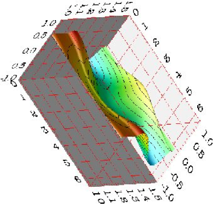
(a) (b)

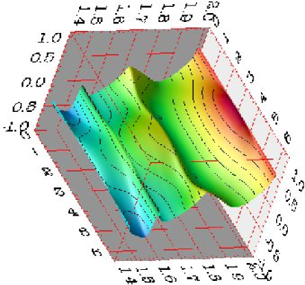
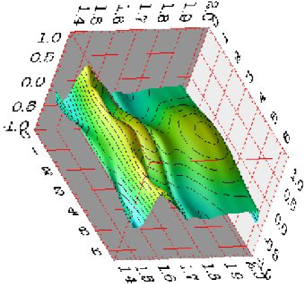
(c) (d)

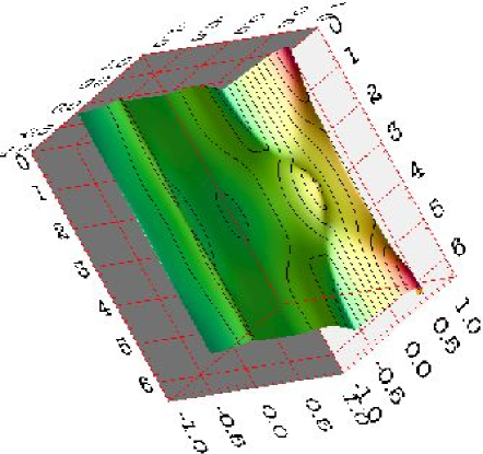
Figure 5: The observable $I^{s}$, showing its sensitivity to the coupling constants $G_{v}^{\phi}$ and $G_{t}^{\phi}$. (a): $G_{v}^{\phi}=4,\,\,G_{t}^{\phi}=0$; (b): $G_{v}^{\phi}=-4,\,\,G_{t}^{\phi}=0$; (c): $G_{v}^{\phi}=0,\,\,G_{t}^{\phi}=4$; (d): $G_{v}^{\phi}=0,\,\,G_{t}^{\phi}=-4$. In each case, the surface is shown as a function of $m_{K\overline{K}}$ and $\Phi^{*}$.

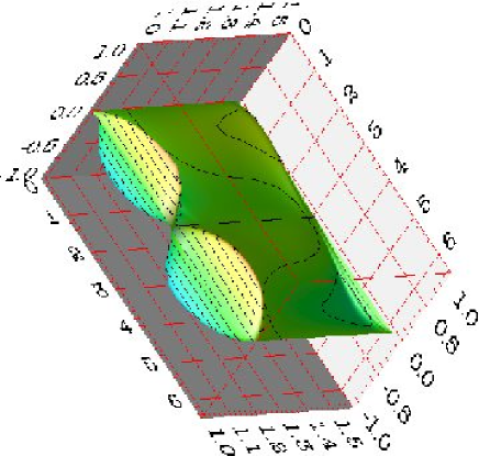
(a) (b)

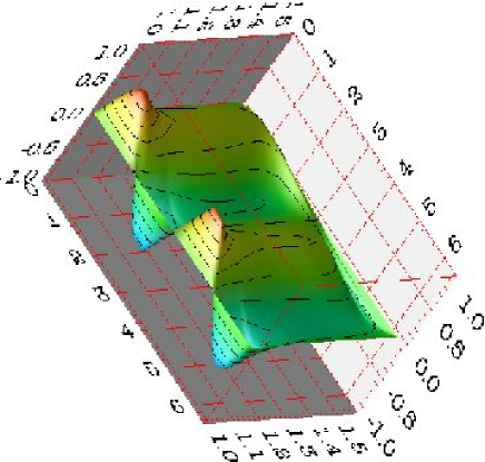
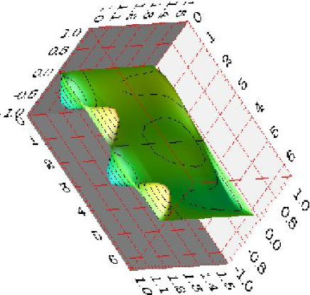
(c) (d)

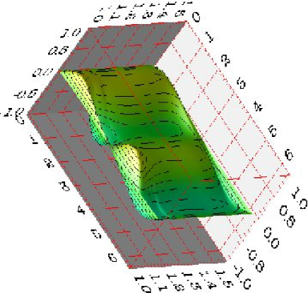
Figure 6: The observable $P_{x}^{\odot}$, showing its sensitivity to the coupling constants $G_{v}^{\phi}$ and $G_{t}^{\phi}$. (a): $G_{v}^{\phi}=4,\,\,G_{t}^{\phi}=0$; (b): $G_{v}^{\phi}=-4,\,\,G_{t}^{\phi}=0$; (c): $G_{v}^{\phi}=0,\,\,G_{t}^{\phi}=4$; (d): $G_{v}^{\phi}=0,\,\,G_{t}^{\phi}=-4$. In each case, the surface is shown as a function of $m_{K\overline{K}}$ and $\Phi^{*}$.

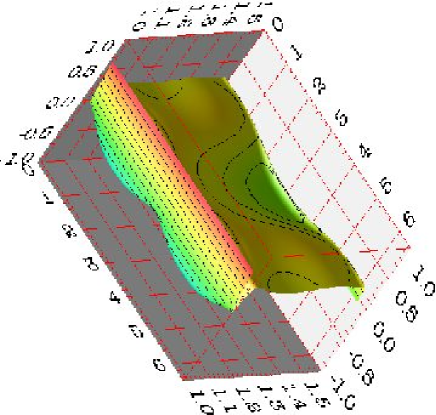
(a) (b)

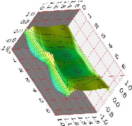
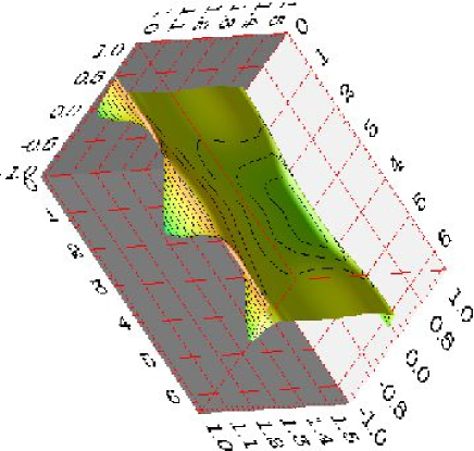
(c) (d)

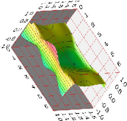
Figure 7: The observable $P_{x}^{s}$, showing its sensitivity to the sub-threshold resonance $\Lambda(1405)$. (a) results with the $\Lambda(1405)$ included in the calculation. (b) results when this state is excluded. Both surfaces are shown as functions of $m_{N\overline{K}}$ and $\Phi^{*}$.

(a)

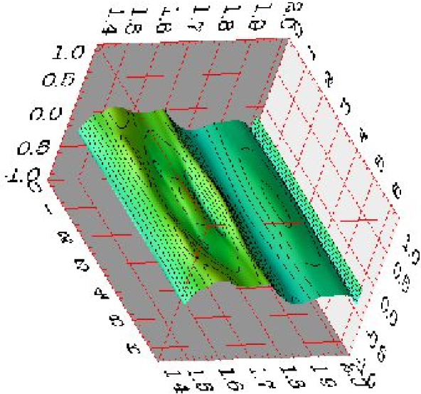
(b)

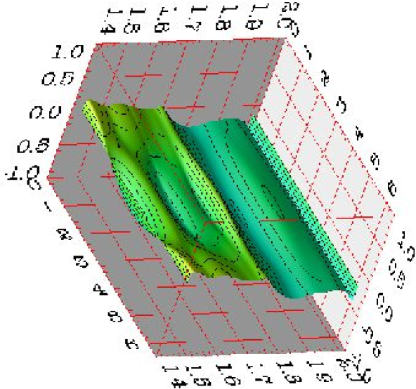
Figure 8: The observable $I^{c}$, showing its sensitivity to the sub-threshold resonance $\Lambda(1405)$. (a) results with the $\Lambda(1405)$ included in the calculation. (b) results when this state is excluded. Both surfaces are shown as functions of $m_{N\overline{K}}$ and $\Phi^{*}$.

(a)

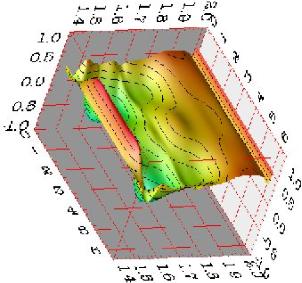
(b)

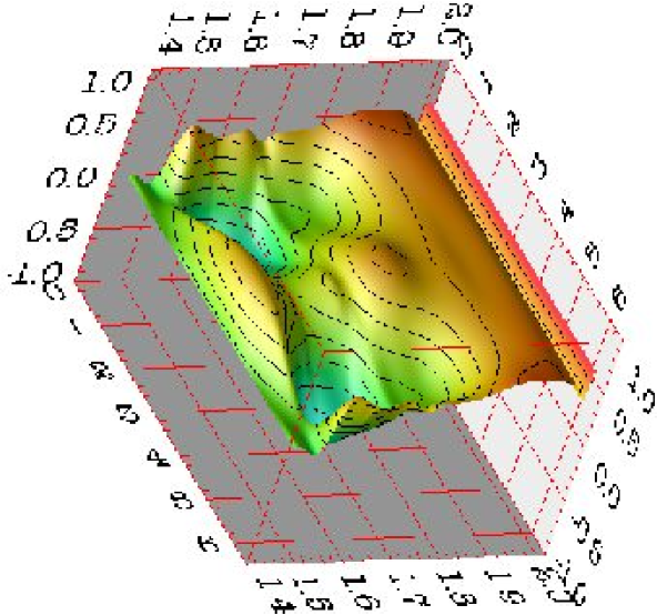
Figure 9: The observable $P_{y}^{c}$, showing its sensitivity to the sub-threshold resonance $\Lambda(1405)$. (a) results with the $\Lambda(1405)$ included in the calculation. (b) results when this state is excluded. Both surfaces are shown as functions of $m_{N\overline{K}}$ and $\Phi^{*}$.

(a)

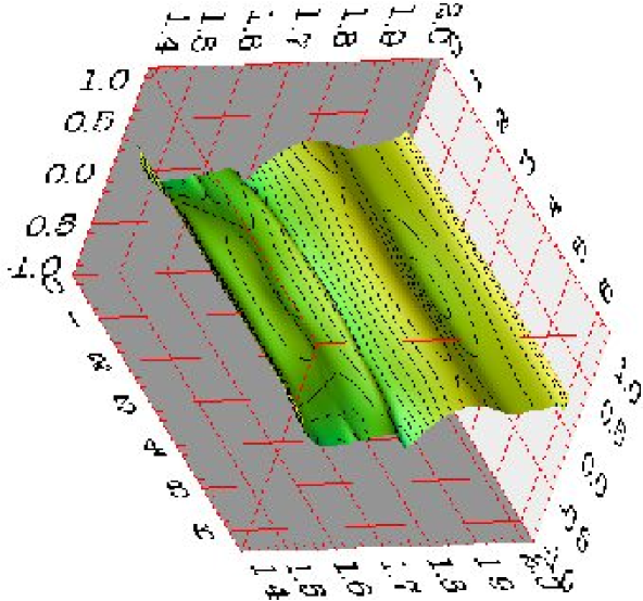
(b)

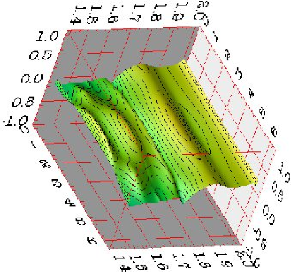
Figure 10: Same as in fig. 9, but with a different view point.

(a)

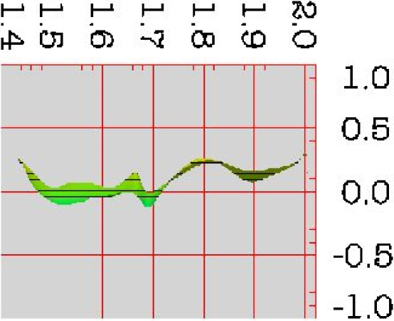
(b)

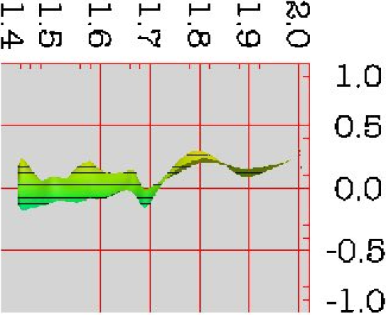
Figure 11: The observable ${\cal O}_{yz^{\prime}}^{c}$, showing its sensitivity to the sub-threshold resonance $\Lambda(1405)$. (a) results with the $\Lambda(1405)$ included in the calculation. (b) results when this state is excluded. Both surfaces are shown as functions of $m_{N\overline{K}}$ and $\Phi^{*}$.

(a)

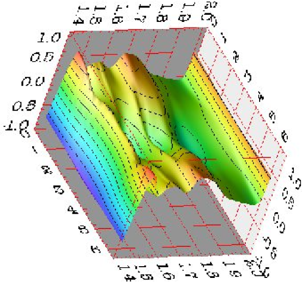
(b)

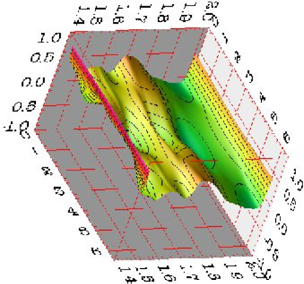
Figure 12: The beam asymmetry, $I^{\odot}$, showing its sensitivity to the exotic resonance $\Theta^{+}$. (a) results with the $\Theta^{+}$ included in the calculation. (b) results when this state is excluded. Both surfaces are shown as functions of $m_{NK}$ and $\Phi^{*}$.

(a)

(b)

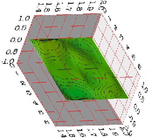
Figure 13: The observable $P^{\odot}_{x}$, showing its sensitivity to the exotic resonance $\Theta^{+}$. (a) results with the $\Theta^{+}$ included in the calculation. (b) results when this state is excluded. Both surfaces are shown as functions of $m_{NK}$ and $\Phi^{*}$.

(a)

(b)

Figure 14: The observable $P^{\odot}_{z}$, showing its sensitivity to the exotic resonance $\Theta^{+}$. (a) results with the $\Theta^{+}$ included in the calculation. (b) results when this state is excluded. Both surfaces are shown as functions of $m_{NK}$ and $\Phi^{*}$.

(a)

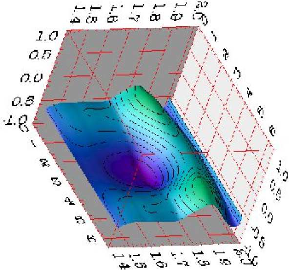
Figure 15: The beam asymmetry, $I^{\odot}$, showing its sensitivity to the parity of the exotic resonance $\Theta^{+}$. (a) results when a $\Theta^{+}$ having $J^{P}=1/2^{+}$ is included. (b) results when this state has $J^{P}=1/2^{-}$. Both surfaces are shown as functions of $m_{NK}$ and $\Phi^{*}$.

(a)

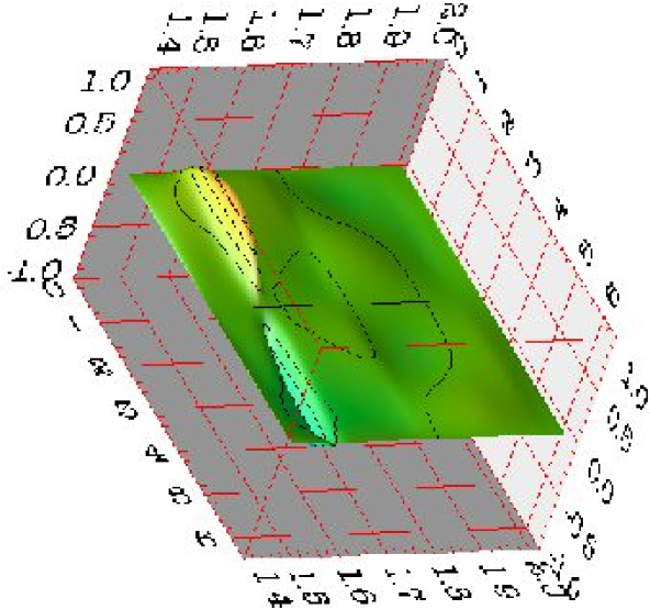
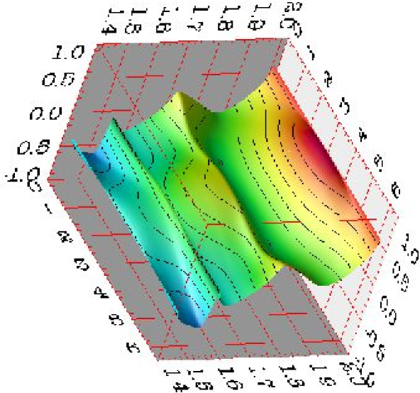
(b)

Figure 16: The observable $P^{\odot}_{x}$, showing its sensitivity to the parity of the exotic resonance $\Theta^{+}$. (a) results when a $\Theta^{+}$ having $J^{P}=1/2^{+}$ is included. (b) results when this state has $J^{P}=1/2^{-}$. Both surfaces are shown as functions of $m_{NK}$ and $\Phi^{*}$.

(a)

(b)

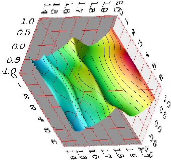
Figure 17: The observable $P^{\odot}_{z}$, showing its sensitivity to the parity of the exotic resonance $\Theta^{+}$. (a) results when a $\Theta^{+}$ having $J^{P}=1/2^{+}$ is included. (b) results when this state has $J^{P}=1/2^{-}$. Both surfaces are shown as functions of $m_{NK}$ and $\Phi^{*}$.

(a)

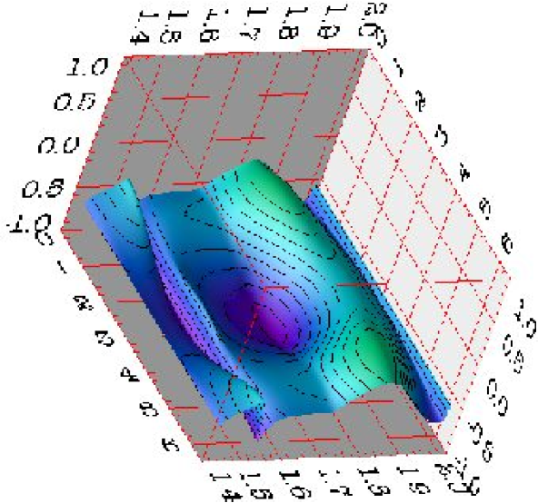
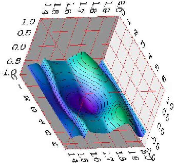
(b)

References

- (1) W. Roberts and T. Oed, nucl-th/0410012, submitted to Physical Review C.
- (2) W. Roberts, nucl-th/0408034, to appear in Physical Review C.
- (3) S. Strauch [CLAS Collaboration], arXiv:nucl-ex/0407008; S. Strauch [CLAS Collaboration], in proceedings of 2nd Conference on Nuclear and Particle Physics with CEBAF at JLab (NAPP 2003), Dubrovnik, Croatia, 26-31 May 2003; manuscript in preparation.
-
(4)
T. Nakano et al. [LEPS Collaboration],
Phys. Rev. Lett. 91, 012002 (2003);
V. Barmin et al. [DIANA Collaboration], Phys. Atom. Nucl. 66, 1715 (2003) [Yad. Fiz. 66, 1763 (2003)];
S. Stepanyan et al. [CLAS Collaboration], Phys. Rev. Lett. 91, 252001 (2003);
J. Barth et al. [SAPHIR Collaboration], Phys. Lett. B 572, 127 (2003);
V. Kubarovsky et al. [CLAS Collaboration], Phys. Rev. Lett. 92, 032001 (2004) [Erratum-ibid. 92, 049902 (2004)];
A. E. Asratyan, A. G. Dolgolenko, and M. A. Kubantsev, Phys. Atom. Nucl. 67, 682 (2004) [Yad. Fiz. 67, 704 (2004)];
A. Airapetian et al. [HERMES Collaboration], Phys. Lett. B 585, 213 (2004);
A. Aleev et al. [SVD Collaboration], hep-ex/0401024;
M. Abdel-Bary et al. [COSY-TOF Collaboration], hep-ex/0403011.