Abstract

Three types of microscopic nucleus-nucleus optical potentials are constructed using three patterns for their real and imaginary parts. Two of these patterns are the real $V^{H}$ and imaginary $W^{H}$ parts of the potential which reproduces the high-energy amplitude of scattering in the microscopic Glauber-Sitenko theory. Another template $V^{DF}$ is calculated within the standard double-folding model with the exchange term included. For either of the three tested potentials, the contribution of real and imaginary patterns is adjusted by introducing two fitted factors. An acceptable agreement with the experimental data on elastic differential cross-sections was obtained for scattering the ^16, 17O heavy-ions at about hundred Mev/nucleon on different target-nuclei. The relativization effect is also studied and found that, to somewhat, it improves the agreement with experimental data.

1 Introduction

One of the main goals of studying heavy-ion scattering remains to obtain the nucleus-nucleus optical (complex) potential. Such a potential is required not only for physical interpretation of experimental data in elastic channel but also to get the optical-model wave functions used in the DWBA calculations of direct inelastic processes and of the nucleons removal reactions. Unfortunately, when fitting data with the help of phenomenological optical potentials one cannot obtain their parameters unambiguously. The other problem is that the parameters of phenomenological potentials depend on the collision energy, atomic numbers and isospins of nuclei. These dependencies present many difficulties in composing appropriate formulae for the global heavy-ion potentials of scattering.

Therefore one ought to follow the more justified way for searching the nucleus-nucleus potentials, namely, to develop the respective microscopic models. In this connection, the attractive and commonly used models are based on the double-folding (DF) procedure, where one calculates integrals with overlapping the density distribution functions of colliding nuclei and the effective nucleon-nucleon potentials (see, e.g., [1, 2, 3]). Moreover, the microscopic models arose considerable interest because they can supply us with underlying effective NN-forces at normal and higher nuclear densities (see, e.g., [4]). This in-medium dependence of NN-potentials is of the great importance in both nuclear- and astro-physics where deeper understanding of e.g. neutron stars and super novae phenomena is needed.

In nucleus-nucleus scattering at energies near and higher the Coulomb barrier, most applications were made by using the optical potential where the real part is calculated within the microscopic model with the direct and exchange terms included, while the imaginary part of the potential is taken in a phenomenological Woods-Saxon form with a three or more adjustable parameters. In this model, say, semi-microscopic model [1, 2, 3], one further free parameter is usually introduced to renormalize the real DF-part of the optical potential. Thus, the general problem still remains when one parametrizes the global dependence of the imaginary part on the potential energy, atomic numbers,… etc.

In the present work, we suggest the method where the pattern potentials are used to compose the microscopic nucleus-nucleus optical potential. As a basis we take the complex potential which fully corresponds to the microscopic high-energy approximation of Glauber and Sitenko [5, 6], being later developed in [7, 8] for deriving the nucleus-nucleus scattering amplitude. This potential (composed of both the real and imaginary parts) depends on energy and uses density distributions of nuclei and the nucleon-nucleon amplitude of scattering with the in-medium effects included. Besides, we take into consideration the microscopic DF-potential, the real one, and use it as a pattern for constructing the full nucleus-nucleus potential. We hope that this regular procedure for obtaining the complex potentials can protect one against the possible non-physical forms of phenomenological potentials obtained in the standard fitting procedure.

In Section 2 the microscopical formulation is presented while Section 3 is devoted to results, discussions, and some conclusions.

2 Microscopic Optical Potentials

To formulate the very complicated many-body scattering problem in terms of an equivalent optical potential one should to appeal not only to its theoretical elegance but also to develop the reliable methods which provide its reasonably simple relation to experimental data. In principle, the optical potential in its general form as is done, e.g., in [9], has a very complicated and nonlocal form. However, one believes that it can be presented in the equivalent local form by using a realistic localized expression for the density matrix. So, below we will test the microscopic nucleus-nucleus energy- and density-dependent optical potential in a compact form as follows:

$$U_{opt}(r)\,=\,N_{r}V(r)\,+\,iN_{im}W(r).$$ (1)

Here the three patterns for both of the real $V(r)$ and imaginary $W(r)$ parts are calculated by using the appropriate microscopic models while the normalizing factors $N_{r}$ and $N_{im}$ are considered as free parameters to be fitted to the experimental data.

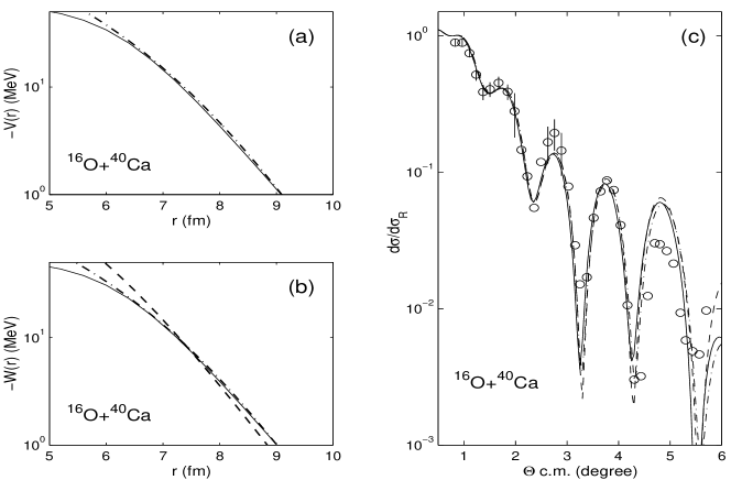
Figure 1: The optical potentials $U_{opt}^{B}$ and $V_{opt}^{C}$ obtained basing on the HEA- and DF-patterns with the fitted $N_{r}$ and $N_{im}$ coefficients (see Table 1A), and the respective ratios of the elastic differential cross-sections to the Rutherford one, for ¹⁶O+⁴⁰Ca at $E_{lab}=$1503 MeV. Panels (a) and (b) are designed for the real and imaginary parts of potentials, where dashed curves are the real and imaginary parts of potentials with the patterns $V^{H}$ (or $W^{H}$), while dash-dotted curves are for those with the patterns $V^{DF}$; the fitted parts of WS-potential from [17] are shown by solid lines. In panel (c), solid curve is calculations with WS-potential, dashed - with $U_{opt}^{B}$, and dash-dotted - with $U_{opt}^{C}$. Open circles – experimental data from [17].

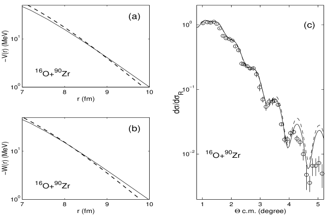
Figure 2: The same as in Fig.1 but for scattering ¹⁶O+⁹⁰Zr with optical potential $U_{opt}^{A}$.

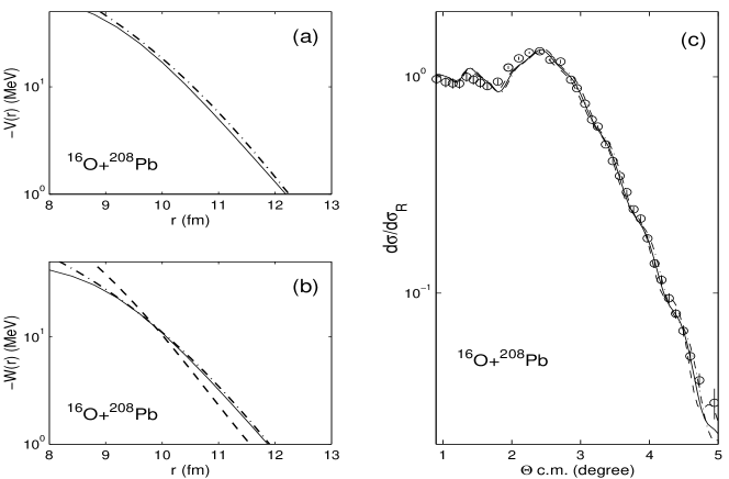
Figure 3: The same as in Fig.1 but for scattering ¹⁶O+²⁰⁸Pb with optical potentials $U_{opt}^{B}$ and $U_{opt}^{C}$.

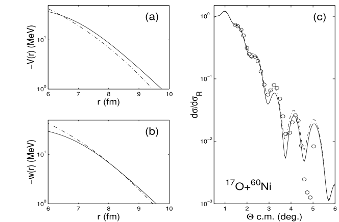
Figure 4: The same as in Fig.1 but for scattering ¹⁷O+⁶⁰Ni at 1435 MeV with optical potential $U_{opt}^{C}$ from Table 1B. Experimental points and the fitted WS-potential are taken from [18].

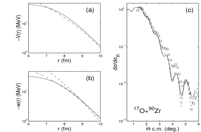
Figure 5: The same as in Fig.4 but for scattering ¹⁷O+⁹⁰Zr with optical potentials $U_{opt}^{B}$ and $U_{opt}^{C}$.

Figure 6: The same as in Fig.4 but for scattering ¹⁷O+¹²⁰Sn with optical potentials $U_{opt}^{B}$ and $U_{opt}^{C}$.

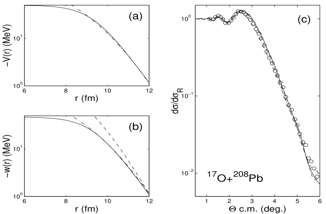
Figure 7: The same as in Fig.4 but for scattering ¹⁷O+²⁰⁸Pb with optical potentials $U_{opt}^{B}$ and $U_{opt}^{C}$.

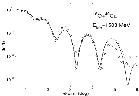
Figure 8: The effect of relativization in case of scattering ¹⁶O+⁴⁰Ca. Solid(dashed) lines show $d\sigma/d\sigma_{R}$  with(without) relativization. The potential $U_{opt}^{C}$ is from Table 1A.

The matter of fact is that, for nucleus-nucleus scattering, the surface region of optical potentials plays a decisive role in predictions of differential and total cross-sections. Concequantly, the usually ensured microscopic models are substantiated namely in this outer region of the collision. Indeed, in a preceding paper [10] a method was developed for the restoration of nucleus-nucleus optical potentials derived on the basis of Glauber-Sitenko microscopic scattering theory where, in the so called optical limit, the microscopic phase was given in the form

$$\Phi_{N}(b)={\bar{\sigma}_{NN}\over 2}(i+{\bar{\alpha}}_{NN})\int d^{2}s_{p}\,d^{2}s_{t}~{}\rho^{\circ}_{p}(s_{p})~{}\rho^{\circ}_{t}(s_{t})~{}f_{N}(|\bf\xi=\bf b+{\bf s}_{p}-{\bf s}_{t}|).$$ (2)

Here $\rho^{\circ}_{p}(r)$ and $\rho^{\circ}_{t}(r)$ are the point nucleon density distributions of the projectile and target nuclei, respectively, and $\rho^{\circ}(s)=\int_{-\infty}^{\infty}\rho^{\circ}(\sqrt{s^{2}+z^{2}})dz$ is the profile function of $\rho^{\circ}(r)$. Also, the function $f_{N}(\xi)=(2\pi)^{-2}\int d^{2}q~{}\exp(-i{\bf q}{\bf\xi}){\tilde{f}}_{N}(q)$ is expressed through the form factor ${\tilde{f}}_{N}(q)$ of the NN-scattering amplitude, taken in the form ${\tilde{f}}_{N}(q)=\exp(-q^{2}r_{N\,rms}^{2}/6)$ with $r_{N\,rms}$, the NN-interaction ${rms}$ radius. Here $\bar{\sigma}_{NN}$ is the total cross section of the NN-scattering while $\bar{\alpha}_{NN}$ is the ratio of the real-to-imaginary part of the forward NN-scattering amplitude, and both of these quantities depend on energy. We denote that the ”bar” means averaging on isotopic spins of colliding nuclei. In [10], this phase (2) was compared with another phenomenological one defined through the optical potential $U(r)=V(r)\,+\,iW(r)$ as follows,

$$\Phi(b)=-\frac{1}{\hbar v}\,\int_{-\infty}^{\infty}U\left(\sqrt{b^{2}+z^{2}}\right)dz,$$ (3)

where $v$ is the relative motion velocity. An analytic expression was used for the phase $\Phi(b)$ of (3), obtained in [11] for the symmetrized Woods-Saxon (SWS) potential, which is the most realistic phenomenological potential often applied in many calculations. The parameters of the SWS-potential were adjusted such that to fit the shape of the phenomenological phase (3) to the microscopic one (2) in the outer region of space $b\sim R_{p}\,+\,R_{t}$. As a result of this procedure it was obtained a set of SWS-potentials which coincide in their tails but have different interiors, and all of them were in a reasonable agreement with elastic scattering differential cross-sections at small angles. Although this method gave surface-equivalent realistic WS-type potentials which means the exclusion of ambiguities in the peripheral region of the interaction, it puts us in face of the traditional old standing ambiguity problem of the optical potentials especially in their internal region.

In such situation, we intend in this work to suggest another approach to restore an optical potential. Towards this aim we believe that the use of microscopic potential models is more reliable in search of a realistic optical potential than fitting a phenomenological one. As a first candidate in this search we suggest to use unambiguous potential that corresponds to the HEA microscopic phase (2). This potential has been obtained independently in [12], by applying the inverse Fourier transform to the HEA-phase (2), and in [13], by substituting the standard expression for the direct DF-potential in the definition of the phase (3). As a result, the so-called HEA-optical potential is as follows:

$$U^{H}_{opt}(r)\,=\,V^{H}(r)\,+\,iW^{H}(r),$$ (4)

where

$$V^{H}(r)=-{2E\over k(2\pi)^{2}}{\bar{\sigma}}_{NN}{\bar{\alpha}}_{NN}\int dq~{}q^{2}j_{0}(qr){\tilde{\rho}^{\circ}}_{p}(q){\tilde{\rho}^{\circ}}_{t}(q){\tilde{f}}_{N}(q),$$ (5)

$$W^{H}(r)=-{2E\over k(2\pi)^{2}}{\bar{\sigma}}_{NN}\int dq~{}q^{2}j_{0}(qr){\tilde{\rho}^{\circ}}_{p}(q){\tilde{\rho}^{\circ}}_{t}(q){\tilde{f}}_{N}(q).$$ (6)

Here ${\tilde{\rho}^{\circ}}_{p(t)}(q)$ are form factors of the corresponding point densities $\rho^{\circ}_{p(t)}(r)$ of the projectile and target nuclei, where the latter functions can be obtained by unfolding the nuclear densities $\rho_{p(t)}(r)$ (see, e.g., [14]), which are usually given in tabulated forms. Thus, the suggested model is free from parameters when calculating the real $V^{H}$ and the imaginary $W^{H}$ parts of the potential. The important and novel point of this method is that it provides to calculate the imaginary part of the potential (6) in a microscopic way. We remind, that in the standard semi-microscopic model one estimates only the real part of the potential using DF-procedure, while the imaginary part is usually taken in a phenomenological WS-form with three or sometimes more fitted parameters. In the present work, in addition to the HEA-potential, we also apply a DF-procedure to estimate the real part of the optical potential, which includes both the direct and exchange terms (see, e.g., [2, 3]):

$$V^{DF}=V^{D}~{}+~{}V^{EX}$$ (7)

where

$$\qquad V^{D}(r)=\int d^{3}r_{p}d^{3}r_{t}\,\rho_{p}({\bf r}_{p})\,\rho_{t}({\bf r}_{t})\,v_{NN}^{D}({\bf r}_{pt}),\quad{\bf r}_{pt}={\bf r}+{\bf r}_{t}-{\bf r}_{p},$$

$$\qquad V^{EX}(r)=\int d^{3}r_{p}d^{3}r_{t}\,\rho_{p}({\bf r}_{p},{\bf r}_{p}+{\bf r}_{pt})\,\rho_{t}({\bf r}_{t},{\bf r}_{t}-{\bf r}_{pt})\times\hskip 113.81102pt$$

$$\hskip 227.62204ptv^{EX}_{NN}({\bf r}_{pt})\,\exp\left[{i{\bf K}(r){\bf r}_{pt}\over M}\right].$$

The dependence on energy in the potential comes from the local relative momentum motion defined as $K(r)\simeq\{2Mm/\hbar^{2}[E-V_{N}(r)-V_{C}(r)]\}^{1/2}$ where $Mm=A_{p}A_{t}m/(A_{p}+A_{t})$ is the reduced mass, E is the relative energy in the center-of-mass frame, and $V_{C}(r)$, the responsible part of the interaction due to the Coulomb potential. We adopt here an energy- and density-dependent version for the effective interaction as given in [3] where the effective interaction $v_{NN}$ is expressed in the form of M3Y force multiplied by the factor $F(\rho)=C[1+\alpha\exp(-\beta\rho)-\gamma\rho]$ which depends on the densities $\rho=\rho_{p}+\rho_{t}$, and also the additional factor $(1-0.003\,E/A_{p})$ is introduced to correct the dependence upon the incident laboratory energy per nucleon.

The comparison between (5) and (7) ensures that the HEA real part $V^{H}$ of the optical potential corresponds only to the direct part $V^{D}$ of the full potential while the $V^{DF}$-real potential consists of two terms, direct and exchange ones, where the latter has a nonlocal nature and arises from the anti-symmetrization between two colliding nuclei, and it accounts for the Pauli-blocking and the so-called knock-on exchange nonlocality. Thus we have two microscopic types of the real potentials $V^{DF}$ and $V^{H}$, and one for the imaginary part $W^{H}$. The HEA-potentials have slightly different slopes in their asymptotics as compared to the DF-potential. In principle, the real and imaginary parts of optical potentials have different physical nature. The first one, as its origin, has the one-particle densities while the second one can get the additional contributions, coming from excitations of collective states and the nucleons removal reactions. Besides, one should bear in mind that at high energies, the peripheral region of the nucleus-nucleus interaction plays the essential role, while the exchange effects reveal themselves mainly in the internal region. At the same time, we pay attention to the result given in [15] that at high energies the nucleons removal reactions mostly contribute to the absorption part of the optical potential while the excitation channels are suppressed. Therefore, one-particle densities take part in equal footing in the formation of both the real and imaginary potentials. Thus, considering not high but intermediate energies of collisions at about 100 MeV/nucleon one can utilize both the shapes HEA- and DF-patterns for composing total microscopic potentials. As a result, we shall test three types of optical potentials, each have only two parameters $N_{r}$ and $N_{im}$, namely:

$$U^{A}_{\scriptsize{opt}}~{}=~{}N^{A}_{r}\,V^{H}~{}+~{}iN^{A}_{im}\,W^{H}$$ (8)

$$U^{B}_{\scriptsize{opt}}~{}=~{}N^{B}_{r}\,V^{DF}~{}+~{}iN^{B}_{im}\,W^{H}$$ (9)

$$U^{C}_{\scriptsize{opt}}~{}=~{}N^{C}_{r}\,V^{DF}~{}+~{}iN^{C}_{im}\,V^{DF}$$ (10)

Usually, in heavy-ion scattering at comparably high energies, the potential tails determine the pattern of the elastic differential cross-sections because of the strong absorption happened at shorter distances. Then, roughly speaking one needs only four parameters to describe the positions and the slope parameters of these tails. In our case we use the microscopic models for both the real and imaginary patterns of the optical potentials given by Eqs.(8)-(10), where by the fitting of only two parameters $N_{r}$ and $N_{im}$ we can, in fact, change the strength and shift of the potential tails in the surface region. In practice, the fit of phenomenological potentials at $E\sim 100$ Mev/nucleon shows that the range from $R_{in}$ to $\infty$ determines the main pattern of the differential cross-sections, and $R_{in}$ is the radius where $V(R_{in})=-50$ Mev. So, below in Figures we show potentials only in this region of their displaying.

3 Results, Discussion, and Conclusions

We calculate the ratio of the elastic differential cross-sections $d\sigma/d\Omega=|f(q)|^{2}$ to the Rutherford cross-section

$${d\sigma_{R}\over d\Omega}\,=\,\left({Z_{p}Z_{t}e^{2}\over\hbar v}\right)^{2}\,{1\over 4k^{2}}\,{1\over\sin^{4}(\vartheta/2)}.$$ (11)

For this purpose we apply the expression for the HEA-scattering amplitude

$$f(q)=ik\int_{0}^{\infty}dbb\,J_{0}(qb)\Bigl{[}1-{\displaystyle e}^{\displaystyle i\Phi_{N}(b)+i\Phi_{C}(b)}\Bigr{]}.$$ (12)

which is valid at $E\gg|U|$ and for small scattering angles $\vartheta<\sqrt{2/kR}$ where $R$ is the nucleus-nucleus interacting radius, say, $R\sim{R_{p}+R_{t}}$. Here $q=2k\sin(\vartheta/2)$ is the momentum transfer. The Coulomb phase $\Phi_{C}(b)$ is taken in an analytic form for the uniformly charged spherical density distribution. The nuclear phase $\Phi_{N}(b)$ is calculated with a help of the optical potentials (8)-(10), using the microscopic HEA- and DF-models. The trajectory distortion in the Coulomb field is taken into account by changing the impact parameter $b$ by $b_{c}=\bar{a}+\sqrt{{\bar{a}}^{2}+b^{2}}$ in all functions of the integrand of (12) with the exception of $\Phi_{C}(b)$; here $b_{c}$ is the distance of closest approach in a Coulomb field, where $\bar{a}=Z_{p}Z_{t}e^{2}/2E_{c.m.}$. Details of calculations of (12) one can find in [16]. In addition, in calculations, we take into account the relativistic kinematics by substituting the respective expressions of velocity $v$ and the c.m. momentum $k$ in (3), (11) and (12) as follows:

$$\hbar v\,=\,197.327\,{\sqrt{E_{l}(E_{l}+2A_{p}m)}\over E_{l}+A_{p}m}\quad(in~{}~{}MeV\,fm),$$ (13)

$$k\,=\,{1\over 197.327}\,\frac{A_{t}\sqrt{E_{l}(E_{l}+2A_{p}m)}}{\sqrt{(A_{p}+A_{t})^{2}\,+\,2A_{t}E_{l}/m}}\quad(in~{}~{}fm^{-1}),$$ (14)

where $E_{l}$ (in MeV) is the kinetic energy of the projectile nucleus in laboratory system, and $m$=931.494 (in MeV) is the unified atomic mass unit.

Below we present our calculations of the cross-section $d\sigma/d\sigma_{R}$ for scattering of ¹⁶O on the targets ⁴⁰Ca, ⁹⁰Zr, and ²⁰⁸Pb at incident energy $E_{l}$=1503 MeV, and ¹⁷O on ⁶⁰Ni, ⁹⁰Zr, ⁹⁰Sn, and ²⁰⁸Pb at $E_{l}$=1435 MeV, and compare these calculations with the corresponding experimental data from Refs. [17] and [18], respectively. The pattern potentials $V^{H},~{}W^{H}$,  and $V^{DF}$ were computed with the help of (4)-(7) using the point density distribution functions $\rho^{\circ}(r)$ for ¹⁶O and respective target-nuclei from [14], and for the corresponding nuclei in collisions of ¹⁷O - from [19] and [20]. Also, parameterization of $\bar{\sigma}_{NN}$ and $\bar{\alpha}_{NN}$ are taken from [21] and [22] while the effective $v_{NN}$-forces of the type CDM3Y6 are obtained from [4]. The normalizing coefficients $N_{r}$ and $N_{im}$ in (8)-(10) were fitted for each couple of colliding nuclei and presented in Tables 1A and 1B.

In Figs.1-7, panels (a) and (b) show the real and imaginary parts of the optical potentials $U_{opt}^{A}$, $U_{opt}^{B}$, and $U_{opt}^{C}$ calculated by using the microscopic models HEA and DF as patterns. Dashed curves represent the potentials with patterns $V^{H}$ and $W^{H}$, while those with $V^{DF}$ are shown by dash-dotted curves. The phenomenological Woods-Saxon (WS) potentials, are shown by solid lines. The ratios of the respective elastic to Rutherford differential cross-sections are presented in panels (c) of Figs.1-7, where dashed curves show the HEA-calculations with the potentials $U_{opt}^{A}$ or $U_{opt}^{B}$, dashed-dotted lines – with the potentials $U_{opt}^{C}$, and solid curves – with the fitted WS-potentials; open circles are the experimental data.

One can see that the slopes of the calculated and the fitted potentials in the outer region have a coincidence to each others. The differential cross-sections fall down by an exponential low beyond the Coulomb rainbow angle, and have an acceptable agreement with the experimental data. As to applicability of the HEA-calculations, we can refer to the sufficient agreements with the experimental data of the HEA cross-sections for the WS-potentials (solid curves). On the other hand, these potentials were obtained by fitting to the same data given in [17] and [18] not by the HEA-calculations but with the help of numerical solutions of the Schroedinger equation. Indeed, this agreement takes place at angles $\vartheta<5.5^{\circ}$ where the HEA is valid by definition. In Tables 1A and 1B the fitted normalizing factors $N_{r}$ and $N_{im}$ of both the real and imaginary parts of the different microscopic optical potentials are demonstrated. In addition, we demonstrate in Fig.8 the relativistic effect on the differential elastic scattering cross-section of ${}^{16}O$+⁴⁰Ca at $E_{l}$=1503 MeV, when one uses the relativistic formulae (13),(14) for $k$ and $v$ in (3),(11), (12). Although this effect is seen not to be large at this energy, the calculated cross-section $d\sigma/d\sigma_{R}$ is in favor of its improvement when compared with its experimental counterpart.

Table 1A.  Optical potentials for the ¹⁶O heavy-ion scattering on different nuclei

$U$	${{}^{16}O}+{{}^{40}Ca}$	${{}^{16}O}+{{}^{90}Zr}$	${{}^{16}O}+{{}^{208}Pb}$
$U^{A}_{opt}$	—	$1.13V^{H}+iW^{H}$	—
$U^{B}_{opt}$	$V^{DF}+i1.32W^{H}$	—	$V^{DF}+iW^{H}$
$U^{C}_{opt}$	$V^{DF}+i0.88V^{DF}$	—	$V^{DF}+i0.6V^{DF}$

Table 1B.  Optical potentials for the ¹⁷O heavy-ion scattering on different nuclei

U	${{}^{17}O}+{{}^{60}Ni}$	${{}^{17}O}+{{}^{90}Zr}$	${{}^{17}O}+{{}^{120}Sn}$	${{}^{17}O}+{{}^{208}Pb}$
$U^{A}_{opt}$	—	—	—	—
$U^{B}_{opt}$	—	$0.6V^{DF}+i0.9W^{H}$	$0.5V^{DF}+i0.9W^{H}$	$0.5V^{DF}+i1.3W^{H}$
$U^{C}_{opt}$	$0.6V^{DF}+i0.6V^{DF}$	$0.6V^{DF}+i0.5V^{DF}$	$0.5V^{DF}+i0.5V^{DF}$	$0.5V^{DF}+i0.8V^{DF}$

Our main conclusion, although we did not intend to achieve a perfect fit as usually experimentalists do, is that the presented idea proves itself to utilize the microscopic models as patterns for further fit with the experimental data. In addition, this method introduce only two adjusted normalizing free parameters instead of, at least, twice that number of parameters required in case of use the phenomenological WS-optical potential. Moreover, at high energy interactions, one can be confident to claim that the results of the calculations done by using the microscopic potentials show that in the outer region of the interactions a true prediction and behavior of these potentials can be gained in the very sensitive domain of the heavy-ion scattering.

ACKNOWLEDGMENTS

The co-authors V.K.L. and B.S. are grateful to the Infeld-Bogoliubov Program for support of this work. One of us E.V.Z. thanks the Russian Foundation Basic Research (project 03-01-00657) for support. Also deep gratitude from K.M. Hanna to the authorities of AEA-Egypt and JINR for their support.

References

- [1] G.R.Satchler G.R. and W.G.Love, Phys.Rep. 55, 183 (1979).
- [2] Dao Tien Khoa and O.M.Knyaz’kov, Phys.El.Part.Nucl. 27, 1456 (1990).
- [3] D.T.Khoa and G.R.Satchler, Nucl.Phys.A 668, 3 (2000).
- [4] D.T.Khoa, G.R.Satchler, and W.von Oertsen, Phys.Rev.C 56, 954 (1997).
- [5] R.J.Glauber, Lectures in Theoretical Physics (N.Y.: Interscience, 1959. P.315).
- [6] A.G.Sitenko, Ukr.Fiz.Zhurn.4, 152 (1959) (in Russian).
- [7] W.Czyz, L.C.Maximon, Ann.of Phys.(N.Y.) 52, 59 (1969).
- [8] J.Formanek, Nucl.Phys.B 12, 441 (1969).
- [9] H.Feshbach, Ann.Phys. 5, 357 (1958);ibid. 19, 287 (1962).
-
[10]
V.K.Lukyanov, E.V.Zemlyanaya, B.Słowiński, and K.Hanna,
Izv.RAN, ser.fiz., 67, no.1, 55 (2003) (in Russian);
K.M.Hanna, V.K.Lukyanov, B.Słowiński,and E.V.Zemlyanaya, Proc.Nucl. Part.Phys.Conf. (NUPPAC’01), Cairo, Egypt (2001) (ed.by M.N.H.Comsan and K.M.Hanna, printed in Cairo by ENPA, 2002, Nasr City 11787), p.121. - [11] V.K.Lukyanov and E.V.Zemlyanaya, J.Phys.G 26, 357 (2000).
- [12] P.Shukla, Phys.Rev.C 67, 054607 (2003).
- [13] V.K.Lukyanov, E.V.Zemlyanaya, and K.V.Lukyanov, Preprint P4-2004-115, JINR, Dubna, 2004.
-
[14]
V.K.Lukyanov, E.V.Zemlyanaya, and B.Słowiński, Yad.Fiz.
67, 1306 (2004)
(in Russian);
V.K.Lukyanov, E.V.Zemlyanaya, and B.Słowiński, Phys.Atom.Nucl. 67, 1282 (2004). - [15] J.H.Sørensen and A.Winther, Nucl.Phys.A 550, 329 (1992).
- [16] V.K.Lukyanov and E.V.Zemlyanaya, Int.J.Mod.Phys.E 10, 169 (2001).
- [17] P. Roussel-Chomaz, et al, Nucl.Phys.A 477, 345 (1988).
- [18] R.Liguori Neto, et al, Nucl.Phys.A 560, 733 (1993).
- [19] J.D.Patterson and R.J.Peterson, Nucl.Phys.A 717, 235 (2003).
- [20] M.El-Azab Farid and G.R.Satchler, Nucl.Phys.A 438, 525 (1985).
- [21] S.K.Charagi and S.K.Gupta, Phys.Rev.C. 41, 1610 (1990).
- [22] P.Shukla, arXiv:nucl-th/0112039.